跳到论文正文
W Papers独立论文阅读器 arXiv:1011.4897 论文正文 计算阅读时间 · 0%
引用这篇论文根据当前论文元数据生成,正式投稿前建议核对。


License: arXiv.org perpetual non-exclusive license
arXiv:1011.4897v2 [math.AG] 28 Nov 2011

Universal covers and the GW/Kronecker correspondence

Jacopo Stoppa Address: Department of Pure Mathematics and Mathematical Statistics, University of Cambridge, Wilberforce Road, Cambridge CB3 0WB, UK Email address: J.Stoppa@dpmms.cam.ac.uk
Abstract.

The tropical vertex is an incarnation of mirror symmetry found by Gross, Pandharipande and Siebert. It can be applied to mm-Kronecker quivers K⁡(m)K(m) (together with a result of Reineke) to compute the Euler characteristics of the moduli spaces of their (framed) representations in terms of Gromov-Witten invariants (as shown by Gross and Pandharipande). In this paper we study a possible geometric picture behind this correspondence, in particular constructing rational tropical curves from subquivers of the universal covering quiver K~​(m)\widetilde{K}(m). Additional motivation comes from the physical interpretation of mm-Kronecker quivers in the context of quiver quantum mechanics (especially work of F. Denef).

1. Introduction

The mm-Kronecker quiver K⁡(m)K(m) is the bipartite quiver with mm edges directed from v1v_{1} (the source) to v2v_{2} (the sink):

v1\textstyle{{v_{1}}\ignorespaces\ignorespaces\ignorespaces\ignorespaces\ignorespaces\ignorespaces\ignorespaces\ignorespaces\ignorespaces\ignorespaces\ignorespaces\ignorespaces\ignorespaces\ignorespaces\ignorespaces\ignorespaces\ignorespaces\ignorespaces\ignorespaces\ignorespaces}e1\scriptstyle{e_{1}}e2\scriptstyle{e_{2}}em−1\scriptstyle{e_{m-1}}em\scriptstyle{e_{m}}⋮\textstyle{\vdots}v2\textstyle{v_{2}}

A stability condition (central charge) for its dimension vectors is specified by a pair of integers (w1,w2)(w_{1},w_{2}). We will always refer to the choice (w1,w2)=(1,0)(w_{1},w_{2})=(1,0). One can then form smooth, projective moduli spaces ℳK⁡(m)s,B​(d)\mathcal{M}^{s,B}_{K(m)}(d) for stable representations of K⁡(m)K(m) with dimension vector dd and a 11-dimensional framing at v1v_{1} (respectively ℳK⁡(m)s,F​(d)\mathcal{M}^{s,F}_{K(m)}(d) for a framing at v2v_{2}, see e.g. [ER] for the general theory). By the results of Engel and Reineke [ER] we have explicit formulae for the topological Euler characteristics χ⁡(ℳK⁡(m)s,B​(d))\chi(\mathcal{M}^{s,B}_{K(m)}(d)) (and also for FF-framings).

Here however we are interested in an alternative and rather surprising way of computing these Euler characteristics, using an incarnation of mirror symmetry known as the tropical vertex of Gross, Pandharipande and Siebert [GPS]. It turns out that computing the generating function

∑k≥0χ⁡(ℳK⁡(m)s,B​(k​a,k​b))​xk​a​yk​b\sum_{k\geq 0}\chi(\mathcal{M}^{s,B}_{K(m)}(ka,kb))x^{ka}y^{kb}

is equivalent to working out a Gromov-Witten theory for a family of algebraic surfaces.

Fix coprime positive integers a,ba,b and let ℙ⁡(a,b,1)\mathbb{P}(a,b,1) be the weighted projective plane (ℂ3∖{0})/ℂ∗(\mathbb{C}^{3}\setminus\{0\})/\mathbb{C}^{*}, with action given by λ⋅(z1,z2,z3)=(λa​z1,λb​z2,λ​z3)\lambda\cdot(z_{1},z_{2},z_{3})=(\lambda^{a}z_{1},\lambda^{b}z_{2},\lambda z_{3}). Its toric fan is given by the duals of the divisors D1,D2,DoutD_{1},D_{2},D_{\textrm{out}} cut out by z1,z2,z3z_{1},z_{2},z_{3}. We denote by D1o,D2o,DoutoD^{o}_{1},D^{o}_{2},D^{o}_{\textrm{out}} the subschemes obtained by removing the three torus fixed points. Also choose length mm ordered partitions Pa,PbP_{a},P_{b} with sizes |Pa|=k​a,|Pb|=k​b|P_{a}|=ka,|P_{b}|=kb for an integer k>0k>0. Then the relevant invariants for us are

Na,b​[(Pa,Pb)]∈ℚN_{a,b}[(P_{a},P_{b})]\in\mathbb{Q}

counting rational curves in the weighted projective plane ℙ⁡(a,b,1)\mathbb{P}(a,b,1) which pass through mm-tuples of distinct points x11,…,xm1x^{1}_{1},\dots,x^{1}_{m} on D1oD^{o}_{1}, respectively x12,…,xm2x^{2}_{1},\dots,x^{2}_{m} on D2oD^{o}_{2}, with multiplicities specified by Pa,PbP_{a},P_{b} and which are tangent to DoutoD^{o}_{\textrm{out}} to order kk. As an example N1,1​(2+1,1+1+1)=3N_{1,1}(2+1,1+1+1)=3 counts plane rational cubics with a prescribed node which pass through 44 other prescribed points, and with DoutD_{\textrm{out}} an inflectional tangent. We refer to [GPS] Sections 0.4 and 6.4 for precise definitions and further examples. The numbers Na,b​[(Pa,Pb)]N_{a,b}[(P_{a},P_{b})] are well defined and independent of the choice of points.

The GW/mm-Kronecker correspondence is the identity in ℚ⁡[[x,y]]\mathbb{Q}[[x,y]]

exp⁡(∑k≥1∑|Pa|=k​a,|Pb|=k​bk​Na,b​[(Pa,Pb)]​xk​a​yk​b)\exp\left(\sum_{k\geq 1}\sum_{|P_{a}|=ka,|P_{b}|=kb}kN_{a,b}[(P_{a},P_{b})]x^{ka}y^{kb}\right)\hskip 113.81102pt
=(1+∑k≥1χ⁡(ℳK⁡(m)s,B​(k​a,k​b))​xk​a​yk​b)ma\hskip 56.9055pt=\left(1+\sum_{k\geq 1}\chi(\mathcal{M}^{s,B}_{K(m)}(ka,kb))x^{ka}y^{kb}\right)^{\frac{m}{a}}
=(1+∑k≥1χ⁡(ℳK⁡(m)s,F​(k​a,k​b))​xk​a​yk​b)mb,\hskip 142.26378pt=\left(1+\sum_{k\geq 1}\chi(\mathcal{M}^{s,F}_{K(m)}(ka,kb))x^{ka}y^{kb}\right)^{\frac{m}{b}}, (1.1)

(summing over length mm ordered partitions Pa,PbP_{a},P_{b}), first written down explicitly by Gross and Pandharipande [GP] Corollary 3.

Gross and Pandharipande [GP] Section 3.5 and Reineke [Re] Section 6 have asked if there is actually a correspondence between curves and representations underlying the equality (1.1). In particular one could ask how to costruct a rational curve starting from a given framed representation of K⁡(m)K(m).

This question was the original motivation for writing this paper. We hoped initially that it would be possible to construct a rational tropical curve starting from a suitable framed representation of the universal covering of the quiver, K~​(m)\widetilde{K}(m) (due to Reineke and Weist). Our hope was motivated by the case of the standard Kronecker quiver K⁡(2)K(2), where we will see that this is roughly true. By the results of Weist [We] (see Theorem 2.1 and (2.3) below) passing to K~​(2)\widetilde{K}(2) is the same as localising with respect to the natural (ℂ∗)2(\mathbb{C}^{*})^{2}-action, so the Euler characteristics can be computed already on K~​(2)\widetilde{K}(2). On the other hand, the GW invariants Na,b​[(Pa,Pb)]N_{a,b}[(P_{a},P_{b})] do arise from certain tropical counts Ntrop​(w)N^{\operatorname{trop}}(\textbf{w}), see [GPS] Theorem 3.4 and Proposition 5.3 (summarized in Theorem 2.74 below).

When m≥3m\geq 3 however this approach becomes problematic and we are not able to construct a single rational tropical curve from a given representation. What we do instead is roughly the following. For a finite subquiver Q⊂K~​(m)Q\subset\widetilde{K}(m) and a “perturbative” parameter k≥1k\geq 1 we construct a whole (finite) set of rational tropical curves 𝒮Q,k\mathcal{S}_{Q,k}. By Weist’s Theorem, representations of QQ embed in representations of K⁡(m)K(m), so we may think of the assignment Q↦𝒮Q,kQ\mapsto\mathcal{S}_{Q,k} as a refinement of the construction in [GPS], where a very similar set of curves arises simply from K⁡(m)K(m). Counting the curves in 𝒮Q,k\mathcal{S}_{Q,k} for k≫1k\gg 1 which satisfy some constraints, with a suitable weight (adapted from the usual tropical multiplicity), expresses the contribution of QQ to χ⁡(ℳK⁡(m)s,B​(d))\chi(\mathcal{M}^{s,B}_{K(m)}(d)) for some dimension vector dd. Constraints on the number of “legs” of our tropical curves correspond to constraints on the dimension vector dd. We denote these ad hoc counts NQtrop​(w)N^{\operatorname{trop}}_{Q}(\textbf{w}). We do not claim that they are genuine tropical invariants, i.e. independent of a crucial choice made in their construction. But via the GW/Kronecker correspondence, we find a posteriori a way to think of NQtrop​(w′)N^{\operatorname{trop}}_{Q}(\textbf{w}^{\prime}) as the contribution of QQ to some genuine invariants Ntrop​(w)N^{\operatorname{trop}}(\textbf{w}).

Here is the plan of the paper. We collect the necessary preliminary notions and results in section 2. In section 2.1 we discuss universal covering quivers and Weist’s Theorem. In section 2.2 we introduce the cornerstone of our approach, Reineke’s Theorem 2.11. The genuine tropical counts Ntrop​(w)N^{\operatorname{trop}}(\textbf{w}) and their connection to the GW invariants Na,b​[(Pa,Pb)]N_{a,b}[(P_{a},P_{b})] are discussed in section 2.6. We first present the construction of tropical curves from subquivers of K~​(m)\widetilde{K}(m) under some very strong assumptions, essentially restricting us to K^​(2)\widehat{K}(2). We do this both because we think that K^​(2)\widehat{K}(2) is a good example and because one has stronger results in this case. The construction takes up sections 2.3, 2.4 and the first part of 2.7. The construction which holds for general mm hinges on the factorization/deformation technique of [GPS], explained in section 2.5, and is done in section 2.7. The numbers NQ,ktrop​(w)N^{\operatorname{trop}}_{Q,k}(\textbf{w}) are defined at the end of that section. In section 3 we present our results connecting the tropical curves obtained from QQ with its contribution to χ⁡(ℳK⁡(m)s,B​(d))\chi(\mathcal{M}^{s,B}_{K(m)}(d)), see especially Corollary 3.15 and Corollary 3.49. Very important additional motivation for the present work came from the paper of F. Denef [De], so we include in section 4 some remarks about quiver quantum mechanics. However our grasp of the necessary physical background is very limited, and our discussion will be hardly satisfactory to the experts. The reader would be well-advised to consult [De].
Acknowledgements. This is an application of some of the ideas in [GPS], [Re] and [We]. It was motivated by conversations with So Okada and Thorsten Weist, and I take this opportunity to thank them. I am also grateful to Hiraku Nakajima, Markus Reineke, Elisa Tenni and Richard Thomas, as well as to RIMS, Kyoto and Trinity College, Cambridge.

2. Preliminary notions and results

2.1. Universal covering quivers

Let QQ be a quiver without closed loops, with vertices Q0Q_{0} and edges Q1Q_{1}. The algebraic torus T:=(ℂ∗)|Q1|T:=(\mathbb{C}^{*})^{|Q_{1}|} acts on the affine spaces of representations RepQ​(d)\textrm{Rep}_{Q}(d) for d∈ℕ​Q0d\in\mathbb{N}Q_{0}, by scaling the linear maps in a representation. Let us write X​(T):=Hom⁡(T,ℂ)≅ℤ​Q1\textrm{X}(T):=\operatorname{Hom}(T,\mathbb{C})\cong\mathbb{Z}Q_{1}, the character group of TT. The abelian universal covering quiver of QQ (due to Reineke, see [We] Section 3) is the quiver Q^\widehat{Q} with vertices Q^0=Q0×X​(T)\widehat{Q}_{0}=Q_{0}\times\textrm{X}(T) and arrows given by

(α,χ):(i,χ)→(j,χ+eα)(\alpha,\chi)\!:(i,\chi)\to(j,\chi+e_{\alpha})

for α:i→j\alpha\!:i\to j in Q1Q_{1} and χ∈X​(T)\chi\in\textrm{X}(T). Here eαe_{\alpha} is the character corresponding to α∈Q1\alpha\in Q_{1}. We say that a dimension vector d^∈ℕ​Q^0\hat{d}\in\mathbb{N}\widehat{Q}_{0} is compatible with d∈ℕ​Q0d\in\mathbb{N}Q_{0} if di=∑χd^i,χd_{i}=\sum_{\chi}\hat{d}_{i,\chi} for all i∈Q0i\in Q_{0}, and we write d^∼d\hat{d}\sim d. There is an action of ℤ​Q1\mathbb{Z}Q_{1} on Q^0\widehat{Q}_{0} defined by λ⋅(i,χ)=(i,χ+λ)\lambda\cdot(i,\chi)=(i,\chi+\lambda), which extends to an action on dimension vectors ℕ​Q^0\mathbb{N}\widehat{Q}_{0} by linearity. In the following we will denote by [d^][\,\hat{d}\,] the equivalence class of d^∈ℕ​Q^0\hat{d}\in\mathbb{N}\widehat{Q}_{0}.

Suppose now that we fix a stability function Θ:ℤ​Q0→ℂ\Theta\!:\mathbb{Z}Q_{0}\to\mathbb{C} and a dimension vector dd for which there are no strictly semistable objects (often we call such dimension vectors coprime). Weist studied the fixed locus for the induced torus action on ℳQs​(d)\mathcal{M}^{s}_{Q}(d), proving the isomorphism

(ℳQs​(d))T≅⋃[d^]∼dℳQ^s​(d^)(\mathcal{M}^{s}_{Q}(d))^{T}\cong\bigcup_{[\,\hat{d}\,]\sim d}\mathcal{M}^{s}_{\widehat{Q}}(\hat{d})

(see [We] Theorem 3.11). In turn each of the moduli spaces ℳQ^s​(d^)\mathcal{M}^{s}_{\widehat{Q}}(\hat{d}) admits a torus action, and this gives rise to a tower of fixed loci, described by representations of iterated abelian covering quivers. We may then ask if for a fixed dd this process stabilizes after a finite number of iterations, and what the iterated fixed locus looks like. Weist gave an answer in terms of the universal covering quiver of QQ.

So let W⁡(Q)W(Q) be the group of words on QQ, generated by arrows and their formal inverses. The universal covering quiver Q~\widetilde{Q} of QQ (see [We] Section 3.4) is the quiver with vertices Q~0=Q0×W⁡(Q)\widetilde{Q}_{0}=Q_{0}\times W(Q) and arrows given by

(α,w):(i,w)→(j,w​α)(\alpha,w)\!:(i,w)\to(j,w\alpha)

for α:i→j\alpha\!:i\to j in Q1Q_{1} and w∈W⁡(Q)w\in W(Q). As in the abelian case we have the notion of a compatible dimension vector d~∈ℕ​Q~0\tilde{d}\in\mathbb{N}\widetilde{Q}_{0} for d∈ℕ​Q0d\in\mathbb{N}Q_{0}, and an action of W⁡(Q)W(Q) on ℕ​Q~0\mathbb{N}\widetilde{Q}_{0} given by w′⋅(i,w)=(i,w​w′)w^{\prime}\cdot(i,w)=(i,ww^{\prime}), with equivalence classes [d~][\,\tilde{d}\,].

Theorem 2.1 (Weist [We] Theorem 3.16).

For a fixed coprime dimension vector dd for QQ the iteration process stabilizes, and the iterated fixed locus can be identified with the disjoint union

⋃[d~]∼dℳQs​(d~).\bigcup_{[\,\tilde{d}\,]\sim d}\mathcal{M}^{s}_{Q}(\tilde{d}). (2.2)

In particular for topological Euler characteristics we get

χ⁡(ℳQs​(d))=∑[d~]∼dχ⁡(ℳQ~s​(d~)).\chi(\mathcal{M}^{s}_{Q}(d))=\sum_{[\,\tilde{d}\,]\sim d}\chi(\mathcal{M}^{s}_{\widetilde{Q}}(\tilde{d})).

For our applications we need a small variant of this result, replacing the coprime condition on dd with the presence of a framing. We only state this for the Kronecker quivers K⁡(m)K(m). A B-framing (respectively F-framing) for a representation of K⁡(m)K(m) is the choice of a 11-dimensional subspace L⊂Vv1L\subset V_{v_{1}} (respectively L⊂Vv2L\subset V_{v_{2}}). Similarly BB or FF framings of a representation of K~​(m)\widetilde{K}(m) are given by 11-dimensional subspaces L⊂V(v1,w)L\subset V_{(v_{1},w)} or L⊂V(v2,w)L\subset V_{(v_{2},w)} for some w∈W⁡(K⁡(m))w\in W(K(m)). There is a natural notion of stability for framed representations, which implies ordinary semistability (we refer to [ER]). The framing rules out strictly semistable objects, so that we have smooth moduli spaces ℳK⁡(m)s,B​(d)\mathcal{M}^{s,B}_{K(m)}(d) and ℳK~​(m)s,(v1,α)​(d~)\mathcal{M}^{s,(v_{1},\alpha)}_{\widetilde{K}(m)}(\tilde{d}) (and similarly for FF framings). Then one can check that the proof of Theorem 2.1 carries over to this framed case, giving for Euler characteristics

χ⁡(ℳK⁡(m)s,B​(d))=∑[d~]∼d∑wχ⁡(ℳK~​(m)s,(v1,w)​(d~)).\chi(\mathcal{M}^{s,B}_{K(m)}(d))=\sum_{[\,\tilde{d}\,]\sim d}\sum_{w}\chi(\mathcal{M}^{s,(v_{1},w)}_{\widetilde{K}(m)}(\tilde{d})). (2.3)

We will often use the crucial fact (see [We] Remark 3.18) that the connected components of K~​(m)\widetilde{K}(m) are given by infinite mm-regular trees with an orientation.

Refer to caption

Figure 1. The universal abelian covering quiver K^​(2)\widehat{K}(2).

Example. The universal covering K~​(2)\widetilde{K}(2) coincides with the universal abelian covering K^​(2)\widehat{K}(2) (see Figure 1).

Figure 2. The universal abelian covering quiver K^​(3)\widehat{K}(3).

Example. The universal abelian covering quiver K^​(3)\widehat{K}(3) is the infinite hexagonal quiver (see Figure 2). The universal covering K~​(3)\widetilde{K}(3) is obtained by opening up all the unoriented cycles in K^​(3)\widehat{K}(3) (see Figure 3).

Refer to caption

Figure 3. The universal covering quiver K~​(3)\widetilde{K}(3).

2.2. Reineke’s theorem

We start by fixing a finite subquiver Q⊂K~​(m)Q\subset\widetilde{K}(m). This is a bipartite quiver, i.e. every vertex is either a source or a sink. We label the sinks by i1,…,isi_{1},\dots,i_{s}, the sources by is+1,…,is+Si_{s+1},\dots,i_{s+S} (so there are ss sinks and SS sources). Notice that in particular QQ has no oriented (or indeed unoriented) cycles, so we can follow Reineke’s convention and fix an order such that ik→il⇒k>li_{k}\to i_{l}\Rightarrow k>l. For our purposes we also need that the order is minimal, in the following sense: we label the sources mapping to i1i_{1} by is+1,…,is+ℓ1i_{s+1},\ldots,i_{s+\ell_{1}}, the sources mapping to i2i_{2} by is+ℓ1+1,…,is+ℓ2i_{s+\ell_{1}+1},\ldots,i_{s+\ell_{2}}, and so on.

A dimension vector dd has a reduction d¯∈ℕ​K​(m)0≅ℕ×ℕ\overline{d}\in\mathbb{N}K(m)_{0}\cong\mathbb{N}\times\mathbb{N} given by

d¯=(∑i>sdi,∑i≤sdi).\overline{d}=\big(\sum_{i>s}d_{i},\sum_{i\leq s}d_{i}\big). (2.4)

We will write Ind⁡d,Ind⁡(d¯)\operatorname{Ind}{d},\operatorname{Ind}(\overline{d}) for the index of a dimension vector and its reduction, i.e. the unique positive integer nn such that dn\frac{d}{n} (respectively d¯n\frac{\overline{d}}{n}) is primitive. Notice that we have Ind⁡(d)≤Ind⁡(d¯)\operatorname{Ind}(d)\leq\operatorname{Ind}(\overline{d}). The central charge (1,0)∈(ℕ​K​(m)0)∗(1,0)\in(\mathbb{N}K(m)_{0})^{*} gives a notion of slope,

μ⁡(d¯′,d¯′′)=d¯′d¯′+d¯′′.\mu(\overline{d}^{\prime},\overline{d}^{\prime\prime})=\frac{\overline{d}^{\prime}}{\overline{d}^{\prime}+\overline{d}^{\prime\prime}}. (2.5)

We fix a notion of slope for dimension vectors of QQ induced from the central charge (1,0)(1,0) on K⁡(m)K(m), namely

μ⁡(d)=∑k>sdk∑kdk.\mu(d)=\frac{\sum_{k>s}d_{k}}{\sum_{k}d_{k}}. (2.6)

The set of dimension vectors with slope μ\mu (together with the trivial representation) forms a subsemigroup (ℕ​Q0)μ⊂ℕ​Q0(\mathbb{N}Q_{0})_{\mu}\subset\mathbb{N}Q_{0}.

The Euler form is a bilinear form on ℤ​Q0\mathbb{Z}Q_{0} defined by

e(d′,d′′)=∑i∈Q0di′di′′−∑α:i→jdi′dj′′,e(d^{\prime},d^{\prime\prime})=\sum_{i\in Q_{0}}d^{\prime}_{i}d^{\prime\prime}_{i}-\sum_{\alpha:i\to j}d^{\prime}_{i}d^{\prime\prime}_{j}, (2.7)

where the second sum is over all arrows from ii to jj. We denote its skew-symmetrization by

⟨d′,d′′⟩=e⁡(d′,d′′)−e⁡(d′′,d′).\langle d^{\prime},d^{\prime\prime}\rangle=e(d^{\prime},d^{\prime\prime})-e(d^{\prime\prime},d^{\prime}). (2.8)

Remark. The form ⟨⋅,⋅⟩\langle\,\cdot,\cdot\rangle is sometimes called the DSZ product in physics terminology. Notice that in our case the product ⟨ik,il⟩\langle i_{k},i_{l}\rangle takes values in {0,±1}\{0,\pm 1\}. A possible source of confusion is that the skew-symmetrised Euler form is denoted by {⋅,⋅}\{\cdot,\cdot\} in Reineke’s notation.
A crucial role is played by a Poisson algebra modelled on QQ,

ℬ=(ℂ​[[xk]]k∈Q0,{⋅,⋅}),\mathcal{B}=(\mathbb{C}[[x_{k}]]_{k\in Q_{0}},\{\,\cdot,\cdot\}),

with Poisson bracket generated by {xk,xl}=⟨k,l⟩​xk​xl\{x_{k},x_{l}\}=\langle k,l\rangle x_{k}x_{l}. For any dimension vector d∈ℕ​Q0d\in\mathbb{N}Q_{0} the Kontsevich-Soibelman Poisson automorphism Td∈Aut⁡(ℬ)T_{d}\in\operatorname{Aut}(\mathcal{B}) (a version of the operators appearing in [KS] Section 1.4) is defined by

Td​(xk)=xk​(1+xd)⟨d,k⟩.T_{d}(x_{k})=x_{k}(1+x^{d})^{\langle d,k\rangle}. (2.9)

The fundamental object for us is the Poisson automorphism of ℬ\mathcal{B} given by

Ti1∘Ti2​⋯∘Tis∘Tis+1∘⋯∘Tis+S.T_{i_{1}}\circ T_{i_{2}}\dots\circ T_{i_{s}}\circ T_{i_{s+1}}\circ\dots\circ T_{i_{s+S}}. (2.10)

By the general theory (see e.g. [GPS] Theorem 1.4) this can be written as a product of Poisson automorphisms attached to each rational nonegative slope, ∏μ←θQ,μ\prod^{\leftarrow}_{\mu}\theta_{Q,\mu}. The symbol ←\leftarrow means we are writing factors in this product in the descending slope order from left to right. Reineke showed that the Poisson automorphisms θQ,μ\theta_{Q,\mu} can be computed in terms of the Euler characteristics of moduli spaces of stable framed representations of QQ.

Theorem 2.11 (Reineke [Re] Theorem 2.1).

We have

θQ,μ​(xj)=xj​∏i∈Q0(θQ,μ,i​(x))⟨i,j⟩,\theta_{Q,\mu}(x_{j})=x_{j}\prod_{i\in Q_{0}}(\theta_{Q,\mu,i}(x))^{\langle i,j\rangle}, (2.12)

where

θQ,μ,i​(x)=∑d∈(ℕ​Q0)μχ⁡(ℳQs,i​(d))​xd\theta_{Q,\mu,i}(x)=\sum_{d\in(\mathbb{N}Q_{0})_{\mu}}\chi(\mathcal{M}^{s,i}_{Q}(d))\,x^{d} (2.13)

and ℳQs,i​(d)\mathcal{M}^{s,i}_{Q}(d) is the moduli space of stable representations of QQ (with respect to the choice of slope (2.6)) with a 11-dimensional framing at i∈Q0i\in Q_{0}.

Remark. While we are only concerned with finite subquivers of K~​(m)\widetilde{K}(m) we should make it clear that Reineke’s result holds for general finite quivers without oriented cycles.

2.3. Sorting diagrams

We will be concerned with an iterative process which sorts the factor of the fundamental product (2.10) in the opposite slope order, possibly introducing new factors at each step. This process is encoded by sorting diagrams. Here we give a definition inspired by that of the scattering diagrams appearing in [GPS] Section 1.4. For the sake of exposition, we initially make very strong assumptions about (2.10), and give examples of sorting diagrams which these hold. The restrictive assumptions will be removed in the section 2.5 by working over more general base rings.

So to a fixed product (2.10) we associate a unique sequence of sorting diagrams 𝔖i,i≥0\mathfrak{S}^{i},i\geq 0. These are simply ordered sequences of group elements σji∈ℬ\sigma^{i}_{j}\in\mathcal{B},

𝔖i=(σ1i,…,σℓii).\mathfrak{S}^{i}=(\sigma^{i}_{1},\dots,\sigma^{i}_{\ell_{i}}). (2.14)

We set

𝔖0=(Ti1,Ti2,…​Tis,Tis+1,…​Tis+S).\mathfrak{S}^{0}=(T_{i_{1}},T_{i_{2}},\dots T_{i_{s}},T_{i_{s+1}},\dots T_{i_{s+S}}). (2.15)

Notice that for all elements of 𝔖0\mathfrak{S}^{0} we have a well defined notion of slope: since σj0=Tij\sigma^{0}_{j}=T_{i_{j}} we set μ⁡(σj0)=μ⁡(ij)\mu(\sigma^{0}_{j})=\mu(i_{j}). We define the 𝔖i\mathfrak{S}^{i} for i>0i>0 inductively as follows. We move along the sequence 𝔖i\mathfrak{S}^{i} starting from the left until we meet a pair of group elements with μ⁡(σpi)<μ⁡(σp+1i)\mu(\sigma^{i}_{p})<\mu(\sigma^{i}_{p+1}). We wish to commute σpi\sigma^{i}_{p} past the elements to its right until we meet again an element with smaller slope, μ⁡(σpi)≥μ⁡(σqi)\mu(\sigma^{i}_{p})\geq\mu(\sigma^{i}_{q}).

Assumption 1. Our first (very restrictive) assumption is that for p+1≤p′≤q−1p+1\leq p^{\prime}\leq q-1 we have

(σp′i)−1​σpi​σp′i​(σpi)−1=Tdp′(\sigma^{i}_{p^{\prime}})^{-1}\sigma^{i}_{p}\sigma^{i}_{p^{\prime}}(\sigma^{i}_{p})^{-1}=T_{d_{p^{\prime}}} (2.16)

for some dp′∈ℕ​Q0d_{p^{\prime}}\in\mathbb{N}Q_{0} (we follow the convention that T0=1T_{0}=1). Then we define 𝔖i+1\mathfrak{S}^{i+1} by replacing the segment

(σpi,…,σq−1i)(\sigma^{i}_{p},\dots,\sigma^{i}_{q-1})

in 𝔖i\mathfrak{S}^{i} by

(σp+1i,Tdp+1,σp+2i,Tdp+2,…,Tdq−1,σpi).(\sigma^{i}_{p+1},T_{d_{p+1}},\sigma^{i}_{p+2},T_{d_{p+2}},\dots,T_{d_{q-1}},\sigma^{i}_{p}).

In particular μ⁡(σji+1)\mu(\sigma^{i+1}_{j}) is well defined for all σji+1∈𝔖i+1\sigma^{i+1}_{j}\in\mathfrak{S}^{i+1}.

Assumption 2. The sequence of sorting diagrams 𝔖i\mathfrak{S}^{i} stabilizes for i≫1i\gg 1. We write 𝔖∞\mathfrak{S}^{\infty} for the stable sorting diagram.

Assumption 3. Operators in 𝔖∞\mathfrak{S}^{\infty} with the same slope commute.

If σ,τ\sigma,\tau are two operators in 𝔖∞\mathfrak{S}^{\infty} with σ\sigma preceeding τ\tau, we write σ≺τ\sigma\prec\tau.

The following simple lemma is enough to effectively compute sorting diagrams, under their present (restrictive) definition.

Lemma 2.17.

If ⟨d,e⟩=0\langle d,e\rangle=0 then Td∘Te=Te∘TdT_{d}\circ T_{e}=T_{e}\circ T_{d}; and if ⟨d,e⟩=1\langle d,e\rangle=1 then Td∘Te=Te∘Td+e∘TdT_{d}\circ T_{e}=T_{e}\circ T_{d+e}\circ T_{d}.

Proof.

Both equalities can be checked by direct computation, the second is the “pentagon identity” [KS] Section 1.4. ∎

Example. Consider a localization quiver Q1⊂K^​(2)Q_{1}\subset\widehat{K}(2) with underlying graph given by

i1\textstyle{i_{1}}i3\textstyle{{i_{3}}\ignorespaces\ignorespaces\ignorespaces\ignorespaces\ignorespaces\ignorespaces\ignorespaces\ignorespaces}i2\textstyle{i_{2}}

The sorting diagrams 𝔖i\mathfrak{S}^{i} stabilize for i≥2i\geq 2 and we find

𝔖0\displaystyle\mathfrak{S}^{0} =(Ti1,Ti2,Ti3),\displaystyle=(T_{i_{1}},T_{i_{2}},T_{i_{3}}),
𝔖1\displaystyle\mathfrak{S}^{1} =(Ti1,Ti3,Ti2+i3,Ti2),\displaystyle=(T_{i_{1}},T_{i_{3}},T_{i_{2}+i_{3}},T_{i_{2}}),
𝔖2\displaystyle\mathfrak{S}^{2} =(Ti3,Ti1+i3,Ti2+i3,Ti1+i2+i3,Ti1,Ti2).\displaystyle=(T_{i_{3}},T_{i_{1}+i_{3}},T_{i_{2}+i_{3}},T_{i_{1}+i_{2}+i_{3}},T_{i_{1}},T_{i_{2}}).

Example. Consider a localization quiver Q2⊂K^​(2)Q_{2}\subset\widehat{K}(2) with underlying graph given by

i4\textstyle{{i_{4}}\ignorespaces\ignorespaces\ignorespaces\ignorespaces\ignorespaces\ignorespaces\ignorespaces\ignorespaces}i1\textstyle{i_{1}}i2\textstyle{i_{2}}i5\textstyle{{i_{5}}\ignorespaces\ignorespaces\ignorespaces\ignorespaces\ignorespaces\ignorespaces\ignorespaces\ignorespaces}i3\textstyle{i_{3}}

One can check that the sorting diagrams stabilize for i≥6i\geq 6. The first few are given by

𝔖0\displaystyle\mathfrak{S}^{0} =(Ti1,Ti2,Ti3,Ti4,Ti5),\displaystyle=(T_{i_{1}},T_{i_{2}},T_{i_{3}},T_{i_{4}},T_{i_{5}}),
𝔖1\displaystyle\mathfrak{S}^{1} =(Ti1,Ti2,Ti4,Ti5,Ti3+i5,Ti3),\displaystyle=(T_{i_{1}},T_{i_{2}},T_{i_{4}},T_{i_{5}},T_{i_{3}+i_{5}},T_{i_{3}}),
𝔖2\displaystyle\mathfrak{S}^{2} =(Ti1,Ti4,Ti2+i4,Ti5,Ti2+i5,Ti3+i5,Ti2+i3+i5,Ti2,Ti3)\displaystyle=(T_{i_{1}},T_{i_{4}},T_{i_{2}+i_{4}},T_{i_{5}},T_{i_{2}+i_{5}},T_{i_{3}+i_{5}},T_{i_{2}+i_{3}+i_{5}},T_{i_{2}},T_{i_{3}})
𝔖3\displaystyle\mathfrak{S}^{3} =(Ti4,Ti1+i4,Ti2+i4,Ti1+i2+i4,Ti5,Ti2+i5,Ti3+i5,Ti2+i3+i5,Ti1,Ti2,Ti3)\displaystyle=(T_{i_{4}},T_{i_{1}+i_{4}},T_{i_{2}+i_{4}},T_{i_{1}+i_{2}+i_{4}},T_{i_{5}},T_{i_{2}+i_{5}},T_{i_{3}+i_{5}},T_{i_{2}+i_{3}+i_{5}},T_{i_{1}},T_{i_{2}},T_{i_{3}})
𝔖4\displaystyle\mathfrak{S}^{4} =(Ti4,Ti1+i4,Ti2+i4,Ti5,Ti1+i2+i4+i5,Ti2+i5,Ti3+i5,Ti1+i2+i3+i4+i5CLOSE,\displaystyle=(T_{i_{4}},T_{i_{1}+i_{4}},T_{i_{2}+i_{4}},T_{i_{5}},T_{i_{1}+i_{2}+i_{4}+i_{5}},T_{i_{2}+i_{5}},T_{i_{3}+i_{5}},T_{i_{1}+i_{2}+i_{3}+i_{4}+i_{5}},
OPENTi1+i2+i4,Ti2+i3+i5,Ti1,Ti2,Ti3).\displaystyle\,\,\,\,\,\,\,\,\,\,\,T_{i_{1}+i_{2}+i_{4}},T_{i_{2}+i_{3}+i_{5}},T_{i_{1}},T_{i_{2}},T_{i_{3}}).

We also give an example where the present naive definition of sorting diagrams breaks down (i.e. the sorting diagram is undefined for some finite i>1i>1).
Example. Consider a localization quiver Q3⊂K~​(3)Q_{3}\subset\widetilde{K}(3) with underlying graph given by

i5\textstyle{{i_{5}}\ignorespaces\ignorespaces\ignorespaces\ignorespaces\ignorespaces\ignorespaces\ignorespaces\ignorespaces}i1\textstyle{{i_{1}}}i2\textstyle{{i_{2}}}i7\textstyle{\ignorespaces\ignorespaces\ignorespaces\ignorespaces{i_{7}}\ignorespaces\ignorespaces\ignorespaces\ignorespaces}i6\textstyle{{i_{6}}\ignorespaces\ignorespaces\ignorespaces\ignorespaces\ignorespaces\ignorespaces\ignorespaces\ignorespaces}i3\textstyle{{i_{3}}}i4\textstyle{i_{4}}

A tedious but straighforward computation using Lemma 2.17 shows that

𝔖6=(…,Ti1+i2+i3+i5+i6,Ti7,Ti1+i2+i5+i7,Ti2+i3+i6+i7,Ti1+2​i2+i3+i5+i6+i7,…).\mathfrak{S}^{6}=(\dots,T_{i_{1}+i_{2}+i_{3}+i_{5}+i_{6}},T_{i_{7}},T_{i_{1}+i_{2}+i_{5}+i_{7}},T_{i_{2}+i_{3}+i_{6}+i_{7}},T_{i_{1}+2i_{2}+i_{3}+i_{5}+i_{6}+i_{7}},\dots). (2.18)

Set

ξ\displaystyle\xi =i1+i2+i3+i5+i6,\displaystyle=i_{1}+i_{2}+i_{3}+i_{5}+i_{6},
η\displaystyle\eta =i1+2​i2+i3+i5+i6+i7.\displaystyle=i_{1}+2i_{2}+i_{3}+i_{5}+i_{6}+i_{7}.

The slopes of the elements in the displayed segment are {25,1,12,12,37}\{\frac{2}{5},1,\frac{1}{2},\frac{1}{2},\frac{3}{7}\}. Therefore to compute 𝔖7\mathfrak{S}^{7} we should commute TξT_{\xi} past all the other elements in this segment. This works initially since

⟨ξ,i7⟩\displaystyle\langle\xi,i_{7}\rangle =0,\displaystyle=0,
⟨ξ,i1+i2+i5+i7⟩\displaystyle\langle\xi,i_{1}+i_{2}+i_{5}+i_{7}\rangle =0,\displaystyle=0,
⟨ξ,i2+i3+i6+i7⟩\displaystyle\langle\xi,i_{2}+i_{3}+i_{6}+i_{7}\rangle =0,\displaystyle=0,

but at the last step we find

⟨ξ,η⟩=−1.\langle\xi,\eta\rangle=-1.

We claim that the product Tη−1​Tξ​Tη​Tξ−1T^{-1}_{\eta}T_{\xi}T_{\eta}T^{-1}_{\xi} is not given by a single Poisson automorphism TdT_{d} as in (2.16). To see this consider the action of Tξ,TηT_{\xi},T_{\eta} on the subalgebra generated by variables of the form xa​ξ+b​ηx^{a\xi+b\eta}. We write T¯ξ,T¯η\overline{T}_{\xi},\overline{T}_{\eta} for these restricted operators. Products of the form T¯η−1​T¯ξ​T¯η​T¯ξ−1\overline{T}^{\,-1}_{\eta}\overline{T}_{\xi}\overline{T}_{\eta}\overline{T}^{\,-1}_{\xi} are studied in [KS] Section 1.4. It is shown there that there is a slope-ordered expansion

T¯ξ​T¯η=T¯η​∏a,b→T¯a​η+b​ξΩ⁡(a,b)​T¯ξ\overline{T}_{\xi}\overline{T}_{\eta}=\overline{T}_{\eta}\prod^{\to}_{a,b}\overline{T}^{\Omega(a,b)}_{a\eta+b\xi}\,\overline{T}_{\xi} (2.19)

for certain Ω⁡(a,b)∈ℚ\Omega(a,b)\in\mathbb{Q}, which are nonzero for infinitely many values of (a,b)(a,b) as soon as ⟨ξ,η⟩≤−1\langle\xi,\eta\rangle\leq-1 or ⟨ξ,η⟩≥2\langle\xi,\eta\rangle\geq 2. As observed by Kontsevich and Soibelman, a closed formula for the Ω⁡(a,b)\Omega(a,b) for ⟨ξ,η⟩≤−1\langle\xi,\eta\rangle\leq-1 is not yet known. The first few terms are given by

T¯ξ​T¯η≈T¯η​T¯3​ξ+η−1​T¯2​ξ+η​T¯3​ξ+2​η2​T¯ξ+η−1​T¯2​ξ+2​η−2​T¯2​ξ+3​η2​T¯ξ+2​η​T¯ξ+3​η−1​T¯ξ.\overline{T}_{\xi}\overline{T}_{\eta}\approx\overline{T}_{\eta}\overline{T}^{\,-1}_{3\xi+\eta}\overline{T}_{2\xi+\eta}\overline{T}^{2}_{3\xi+2\eta}\overline{T}^{\,-1}_{\xi+\eta}\overline{T}^{\,-2}_{2\xi+2\eta}\overline{T}^{2}_{2\xi+3\eta}\overline{T}_{\xi+2\eta}\overline{T}^{\,-1}_{\xi+3\eta}\overline{T}_{\xi}. (2.20)

This is enough to show that our present definition of sorting diagrams is too weak in general. There is however a special case when it (almost) works, that of the (abelian) universal covering quiver K~​(2)≅K^​(2)\widetilde{K}(2)\cong\widehat{K}(2).

Lemma 2.21.

Let Q⊂K^​(2)Q\subset\widehat{K}(2) be a finite subquiver. Then the sorting diagrams 𝔖i\mathfrak{S}^{i} exist for all i≥0i\geq 0 and stabilize for i≫1i\gg 1 to a stable diagram 𝔖∞\mathfrak{S}^{\infty}. Moreover operators in 𝔖∞\mathfrak{S}^{\infty} having the same slope μ≠12\mu\neq\frac{1}{2} commute.

Proof.

Let dd be any dimension vector for QQ. Recall that the moduli space of stable representations ℳQs​(d)\mathcal{M}^{s}_{Q}(d), when not empty, has dimension

1−e⁡(d,d).1-e(d,d). (2.22)

In our case of Q⊂K^​(2)Q\subset\widehat{K}(2) it is not hard to show, by induction, that the Euler form e⁡(d,d)e(d,d) is a positive definite quadratic form. It follows that the moduli space ℳQs​(d)\mathcal{M}^{s}_{Q}(d) must be empty for all but finitely many dd. In fact we even have e⁡(d,d)>1e(d,d)>1 if di>1d_{i}>1 for some i∈Q0i\in Q_{0}.

Suppose then that to form some sorting diagram 𝔖i\mathfrak{S}^{i} for QQ we must commute some operator Td′T_{d^{\prime}} past Td′′T_{d^{\prime\prime}} with ⟨d′,d′′⟩∉{0,1}\langle d^{\prime},d^{\prime\prime}\rangle\notin\{0,1\}. Then according to [KS] Section 1.4, the ordered product expansion for Td′′−1∘Td′∘Td′′∘Td′−1T^{-1}_{d^{\prime\prime}}\circ T_{d^{\prime}}\circ T_{d^{\prime\prime}}\circ T^{-1}_{d^{\prime}} must contain infinitely many factors TdT_{d} with distinct slopes, μ⁡(d′)<μ⁡(d)<μ⁡(d′′)\mu(d^{\prime})<\mu(d)<\mu(d^{\prime\prime}). Therefore by Reineke’s Theorem 2.11 there must exist nonempty moduli spaces of (BB or FF) framed representations for infinitely many dd with distinct slopes. Since framed stability implies semistability, the moduli spaces ℳQs​s​(d)\mathcal{M}^{ss}_{Q}(d) must by nonempty for infinitely many dd with distinct slopes. By the Jordan-Holder filtration, there also exist infinitely many distinct nonempty moduli spaces ℳQs​(d∗)\mathcal{M}^{s}_{Q}(d^{*}) for some dimension vectors d∗d^{*}, which is a contradiction. This shows that the 𝔖i\mathfrak{S}^{i} exist for all i≥1i\geq 1. Suppose that the 𝔖i\mathfrak{S}^{i} do not stabilize for i≫1i\gg 1. Then for i≫1i\gg 1 the diagram 𝔖i\mathfrak{S}^{i} must contain an operator TdT_{d} with

d=∑i∈Adi+∑j∈Bdjd=\sum_{i\in A}d_{i}+\sum_{j\in B}d_{j} (2.23)

where A,BA,B are distinct subsets of Q0Q_{0} with A∩B≠∅A\cap B\neq\emptyset. In particular dd is coprime, so the appeareance of TdT_{d} implies that ℳQs​(d)\mathcal{M}^{s}_{Q}(d) in nonempty. But for some i∈Q0i\in Q_{0} we have di=2d_{i}=2, which again contradicts the dimension formula (2.22).

Notice that we have actually proved a much stronger result: all the operators appearing in 𝔖∞\mathfrak{S}^{\infty} must be of the form TdT_{d} for d=∑i∈Aid=\sum_{i\in A}i, where AA is some nonempty subset of Q0Q_{0}. Moreover, by (framed) stability, the support of the dimension vector dd must be connected.

It follows that for two dimension vectors d′,d′′d^{\prime},d^{\prime\prime} with the same slope μ≠12\mu\neq\frac{1}{2}, the number of sources (respectively sinks) in d′d^{\prime} and d′′d^{\prime\prime} is the same (this is clearly not true for μ=12\mu=\frac{1}{2}). Suppose d′=∑i∈Aid^{\prime}=\sum_{i\in A}i, d′′=∑j∈Bjd^{\prime\prime}=\sum_{j\in B}j. We can easily reduce to the case when A∩B=∅A\cap B=\emptyset, and in this latter case there are obviously no arrows from the support of d′d^{\prime} to that of d′′d^{\prime\prime}, so ⟨d′,d′′⟩=0\langle d^{\prime},d^{\prime\prime}\rangle=0. Therefore Td′,Td′′T_{d^{\prime}},T_{d^{\prime\prime}} commute. ∎

Remark. It is easy to show by example that we may have [Td′,Td′′]≠1[T_{d^{\prime}},T_{d^{\prime\prime}}]\neq 1 when μ⁡(d′)=μ⁡(d′′)=12\mu(d^{\prime})=\mu(d^{\prime\prime})=\frac{1}{2}. This difficulty is related to the fact that the moduli spaces of stable framed representations of dimension vector (n,n)(n,n) are nonempty for all nn, namely ℳK⁡(2)s,B​(n,n)≅ℙn\mathcal{M}^{s,B}_{K(2)}(n,n)\cong\mathbb{P}^{n}. We do not address this problem in the special example of K⁡(2)K(2): it will be solved automatically when working over the more general base rings of section 2.5.

Let us also write down for later use the generating series of the Euler characteristics of stable BB-framed representations for K⁡(2)K(2). In fact the only possible dimension vectors are those proportional to one of (a,a+1),(1,1)(a,a+1),(1,1) or (a+1,a)(a+1,a) for a≥1a\geq 1 (see e.g. [GP] Lemma 2.3), and we have (see e.g. [GP] Section 1.4 and Theorem 1)

Ba,a+1\displaystyle B_{a,a+1} =∑k≥1χ⁡(ℳK⁡(2)s,B)​xk​a​yk⁡(a+1)=(1+xa​ya+1)a,\displaystyle=\sum_{k\geq 1}\chi(\mathcal{M}^{s,B}_{K(2)})x^{ka}y^{k(a+1)}=(1+x^{a}y^{a+1})^{a}, (2.24)
B1,1\displaystyle B_{1,1} =∑k≥1χ⁡(ℳK⁡(2)s,B)​xk​yk=(1−x​y)−2,\displaystyle=\sum_{k\geq 1}\chi(\mathcal{M}^{s,B}_{K(2)})x^{k}y^{k}=(1-xy)^{-2}, (2.25)
Ba+1,a\displaystyle B_{a+1,a} =∑k≥1χ⁡(ℳK⁡(2)s,B)​xk⁡(a+1)​yk​a=(1+xa+1​ya)a+1.\displaystyle=\sum_{k\geq 1}\chi(\mathcal{M}^{s,B}_{K(2)})x^{k(a+1)}y^{ka}=(1+x^{a+1}y^{a})^{a+1}. (2.26)

So the generating series are just polynomials in x,yx,y, except for B1,1B_{1,1}.

2.4. Sorting trees

Assumption 1 and 2 say that the sorting diagrams 𝔖i\mathfrak{S}^{i} are well defined and stabilize. Assumption 3 says that it is easy to compose operators with the same slope in the stable sorting diagram 𝔖∞\mathfrak{S}^{\infty}. We now spell out a further condition, which allows us to associate a tree Γ¯σ\overline{\Gamma}_{\sigma} with each element σ∈𝔖i\sigma\in\mathfrak{S}^{i}. Again we will see that this assumption holds automatically when we work over the more general base rings of the next section. Our definition follows that of the tree underlying the scattering diagrams of [GPS] Section 1.4.

Suppose that σ∈𝔖i\sigma\in\mathfrak{S}^{i} arises as the commutator of σ1,σ2∈𝔖i−1\sigma_{1},\sigma_{2}\in\mathfrak{S}^{i-1}. We define

Parents⁡(σ)={σ1,σ2}.\operatorname{Parents}(\sigma)=\{\sigma_{1},\sigma_{2}\}. (2.27)

We then have the recursive functions

Ancestors⁡(σ)={σ}∪⋃σ′∈Parents⁡(σ)Ancestors⁡(σ′)\operatorname{Ancestors}(\sigma)=\{\sigma\}\cup\bigcup_{\sigma^{\prime}\in\operatorname{Parents}(\sigma)}\operatorname{Ancestors}(\sigma^{\prime}) (2.28)

and

Leaves⁡(σ)={σ′∈Ancestors⁡(σ):σ′∈𝔖0}.\operatorname{Leaves}(\sigma)=\{\sigma^{\prime}\in\operatorname{Ancestors}(\sigma):\sigma^{\prime}\in\mathfrak{S}^{0}\}. (2.29)

Assumption 4. If σ′∈Ancestors⁡(σ)∖{σ}\sigma^{\prime}\in\operatorname{Ancestors}(\sigma)\setminus\{\sigma\}, then σ′\sigma^{\prime} is parent to a unique element of Ancestors⁡(σ)\operatorname{Ancestors}(\sigma). We denote this by Child⁡(σ′)\operatorname{Child}(\sigma^{\prime}).
Example. Going back to our examples in the previous section, we see that again this assumption holds in the first two cases of Q1,Q2Q_{1},Q_{2}, and fails for the subquiver Q3⊂K~​(3)Q_{3}\subset\widetilde{K}(3) that we considered. This is because 𝔖7\mathfrak{S}^{7} contains the element Tη=Ti1+2​i2+i3+i5+i6+i7T_{\eta}=T_{i_{1}+2i_{2}+i_{3}+i_{5}+i_{6}+i_{7}}. Then clearly Ti2T_{i_{2}} must be parent to two different ancestors of TηT_{\eta} (a little computation shows that these are in fact Ti2+i5,Ti2+i7T_{i_{2}+i_{5}},T_{i_{2}+i_{7}}).

As before, Assumption 4 holds for subquivers of K^​(2)\widehat{K}(2) without the need to pass to more general base rings.

Lemma 2.30.

Let Q⊂K^​(2)Q\subset\widehat{K}(2) be a finite subquiver and let σ\sigma be an element of some sorting diagram 𝔖i\mathfrak{S}^{i}. If σ′∈Ancestors⁡(σ)∖{σ}\sigma^{\prime}\in\operatorname{Ancestors}(\sigma)\setminus\{\sigma\}, then σ′\sigma^{\prime} is parent to a unique element of Ancestors⁡(σ)\operatorname{Ancestors}(\sigma).

Proof.

If there is σ′∈Ancestors⁡(σ)\sigma^{\prime}\in\operatorname{Ancestors}(\sigma) violating Assumption 4, then we can actually choose σ′=Tip\sigma^{\prime}=T_{i_{p}} for some ip∈Q0i_{p}\in Q_{0}. It follows that for some i>0i>0, 𝔖i\mathfrak{S}^{i} contains an element of the form TdA+dBT_{d_{A}+d_{B}} for some dimension vectors of the form dA=∑i′∈Ai′d_{A}=\sum_{i^{\prime}\in A}i^{\prime}, dB=∑i′′∈Bi′′d_{B}=\sum_{i^{\prime\prime}\in B}i^{\prime\prime} for some distinct A,B⊂Q0A,B\subset Q_{0} with ip∈A∩Bi_{p}\in A\cap B. As before this contradicts the dimension formula (2.22). ∎

Under Assumption 4, we proceed to construct the tree Γ¯σ\overline{\Gamma}_{\sigma}. Both the vertices and edges of Γ¯σ\overline{\Gamma}_{\sigma} are parametrized by ancestors of σ\sigma:

Γ¯σ[0]\displaystyle\overline{\Gamma}^{[0]}_{\sigma} ={Vσ′:σ′∈Ancestors⁡(σ)},\displaystyle=\{V_{\sigma^{\prime}}:\sigma^{\prime}\in\operatorname{Ancestors}(\sigma)\}, (2.31)
Γ¯σ[1]\displaystyle\overline{\Gamma}^{[1]}_{\sigma} ={Eσ′:σ′∈Ancestors⁡(σ)∖{σ}}.\displaystyle=\{E_{\sigma^{\prime}}:\sigma^{\prime}\in\operatorname{Ancestors}(\sigma)\setminus\{\sigma\}\}. (2.32)

Then for σ′∈Ancestors⁡(σ)∖{σ}\sigma^{\prime}\in\operatorname{Ancestors}(\sigma)\setminus\{\sigma\} the vertices of Eσ′E_{\sigma^{\prime}} are {Vσ′,VChild⁡(σ′)}\{V_{\sigma^{\prime}},V_{\operatorname{Child}(\sigma^{\prime})}\}.
Example. Going back to our two examples for K^​(2)\widehat{K}(2) in the previous section, the tree for Γ¯Ti1+i2+i3\overline{\Gamma}_{T_{i_{1}+i_{2}+i_{3}}} in Q1Q_{1} is given by

Ti2\textstyle{{T_{i_{2}}}\ignorespaces\ignorespaces\ignorespaces\ignorespaces}Ti3\textstyle{{T_{i_{3}}}\ignorespaces\ignorespaces\ignorespaces\ignorespaces}Ti2+i3\textstyle{{T_{i_{2}+i_{3}}}\ignorespaces\ignorespaces\ignorespaces\ignorespaces}Ti1\textstyle{{T_{i_{1}}}\ignorespaces\ignorespaces\ignorespaces\ignorespaces}Ti1+i2+i3\textstyle{{T_{i_{1}+i_{2}+i_{3}}}}

while the tree Γ¯Ti1+i2+i3+i4+i5\overline{\Gamma}_{T_{i_{1}+i_{2}+i_{3}+i_{4}+i_{5}}} in Q2Q_{2} is

Ti2\textstyle{T_{i_{2}}\ignorespaces\ignorespaces\ignorespaces\ignorespaces}Ti4\textstyle{T_{i_{4}}\ignorespaces\ignorespaces\ignorespaces\ignorespaces}Ti1\textstyle{T_{i_{1}}\ignorespaces\ignorespaces\ignorespaces\ignorespaces}Ti2+i4\textstyle{{T_{i_{2}+i_{4}}}\ignorespaces\ignorespaces\ignorespaces\ignorespaces}Ti3\textstyle{T_{i_{3}}\ignorespaces\ignorespaces\ignorespaces\ignorespaces}Ti5\textstyle{T_{i_{5}}\ignorespaces\ignorespaces\ignorespaces\ignorespaces}Ti1+i2+i4\textstyle{{T_{i_{1}+i_{2}+i_{4}}}\ignorespaces\ignorespaces\ignorespaces\ignorespaces}Ti3+i5\textstyle{{T_{i_{3}+i_{5}}}\ignorespaces\ignorespaces\ignorespaces\ignorespaces}Ti1+i2+i3+i4+i5\textstyle{{T_{i_{1}+i_{2}+i_{3}+i_{4}+i_{5}}}}

We also define a related unbounded tree Γσ\Gamma_{\sigma}. We set

Γσ[0]\displaystyle\Gamma^{[0]}_{\sigma} ={Vσ′:σ′∈Ancestors⁡(σ)∖𝔖0},\displaystyle=\{V_{\sigma^{\prime}}:\sigma^{\prime}\in\operatorname{Ancestors}(\sigma)\setminus\mathfrak{S}^{0}\}, (2.33)
Γσ[1]\displaystyle\Gamma^{[1]}_{\sigma} ={Eσ′:σ′∈Ancestors⁡(σ)}.\displaystyle=\{E_{\sigma^{\prime}}:\sigma^{\prime}\in\operatorname{Ancestors}(\sigma)\}. (2.34)

For σ′∈Ancestors⁡(σ)∖({σ}∪𝔖0)\sigma^{\prime}\in\operatorname{Ancestors}(\sigma)\setminus(\{\sigma\}\cup\mathfrak{S}^{0}), the vertices of Eσ′E_{\sigma^{\prime}} are defined as {Vσ′,VChild⁡(σ′)}\{V_{\sigma^{\prime}},V_{\operatorname{Child}(\sigma^{\prime})}\} as before. However, for σ′∈Leaves⁡(σ)\sigma^{\prime}\in\operatorname{Leaves}(\sigma) we define Eσ′E_{\sigma^{\prime}} to be an unbounded edge with the single vertex VChild⁡(σ′)V_{\operatorname{Child}(\sigma^{\prime})}. Similarly we define EσE_{\sigma} to be unbounded, with the single vertex VσV_{\sigma}.

We define the weight on edges wΓσ:Γσ[1]→ℕ>0w_{\Gamma_{\sigma}}\!:\Gamma^{[1]}_{\sigma}\to\mathbb{N}_{>0} as follows. We know that σ′∈Ancestors⁡(σ)\sigma^{\prime}\in\operatorname{Ancestors}(\sigma) is a group element of the form TdT_{d} for some d∈ℕ​Q0d\in\mathbb{N}Q_{0}. Recall that we defined a reduction d¯∈ℕ​K​(m)\overline{d}\in\mathbb{N}K(m). We set

wΓσ​(Eσ′)=Ind⁡(d¯).w_{\Gamma_{\sigma}}(E_{\sigma^{\prime}})=\operatorname{Ind}(\overline{d}). (2.35)

Remark. The reason that we further reduce to d¯\overline{d} is that we will be interested in constucting plane tropical curves from Γσ\Gamma_{\sigma}. Their integral structure is modelled on the rank 2 lattice ℤ​K​(m)0\mathbb{Z}K(m)_{0} rather then the higher rank lattice ℤ​Q0\mathbb{Z}Q_{0}.

2.5. More general base rings

In this section we apply the factorization-deformation technique developed in [GPS] Section 1.4. The main advantage is that our Assumptions 1, 2 and 3 will hold automatically in this context. On the other hand Assumption 4 does not hold in general, but we will see that composing operators in the stable sorting diagram is still reasonably simple. Geometrically, in section 2.7 this will give rise to correction terms coming from disconnected curves.

We introduce auxiliary variables t1,…,ts,ts+1,…,tSt_{1},\dots,t_{s},t_{s+1},\dots,t_{S}, and redefine the Kontsevich-Soibelman operators as elements of the group

Autℂ⁡[[t∙]]⁡ℂ⁡[x1,x1−1​…,xS,xS−1]​[[t∙]],\operatorname{Aut}_{\mathbb{C}[[t_{\bullet}]]}\mathbb{C}[x_{1},x^{-1}_{1}\dots,x_{S},x^{-1}_{S}][[t_{\bullet}]], (2.36)

given by

Td​(xi)=xi​(1+td​xd)⟨d,i⟩,T_{d}(x_{i})=x_{i}(1+t^{d}x^{d})^{\langle d,i\rangle}, (2.37)

for d∈ℕ​Q0d\in\mathbb{N}Q_{0}. Fix an integer k≥1k\geq 1. We will work modulo the ideal

(t1k+1,…,tsk+1,ts+1k+1,…,ts+Sk+1).(t^{k+1}_{1},\dots,t^{k+1}_{s},t^{k+1}_{s+1},\dots,t^{k+1}_{s+S}). (2.38)

The full information of the Kontsevich-Soibelman operators is recovered in the limit k→∞k\to\infty. To make this precise define the ring

Rk=ℂ⁡[[t1,…,ts,ts+1,…,ts+S]]/(t1k+1,…,tsk+1,ts+1k+1,…,ts+Sk+1).R_{k}=\mathbb{C}[[t_{1},\dots,t_{s},t_{s+1},\dots,t_{s+S}]]/(t^{k+1}_{1},\dots,t^{k+1}_{s},t^{k+1}_{s+1},\dots,t^{k+1}_{s+S}). (2.39)

We describe how to pass to a version of the fundamental product (2.10) which plays the same role as the standard scattering diagrams of [GPS] Definition 1.10. Consider the ring

R~k=ℂ[{ui​j,1≤i≤s+S,1≤j≤k}]/(ui​j2,1≤i≤s+S,1≤j≤k).\widetilde{R}_{k}=\mathbb{C}[\{u_{ij},1\leq i\leq s+S,1\leq j\leq k\}]/(u^{2}_{ij},1\leq i\leq s+S,1\leq j\leq k). (2.40)

There is an inclusion Rk↪R~kR_{k}\hookrightarrow\widetilde{R}_{k} induced by

ti↦∑j=1kui​j.t_{i}\mapsto\sum^{k}_{j=1}u_{ij}. (2.41)

We can factor each of the operators TiT_{i} in (2.10) over R~k\widetilde{R}_{k}. First we have the identity in RkR_{k},

log⁡(1+ti​xi)=∑j=1k(−1)j−1j​tij​xij.\log(1+t_{i}x_{i})=\sum^{k}_{j=1}\frac{(-1)^{j-1}}{j}t^{j}_{i}x^{j}_{i}. (2.42)

Now in R~k\widetilde{R}_{k},

tij=∑J⊂{1,…,k},#​J=jj!​∏l∈Jui​l.t^{j}_{i}=\sum_{J\subset\{1,\dots,k\},\#J=j}j!\prod_{l\in J}u_{il}. (2.43)

Therefore

log⁡(1+ti​xi)=∑j=1k∑J⊂{1,…,k},#​J=j(−1)j−1​(j−1)!​∏l∈Jui​l​xij,\log(1+t_{i}x_{i})=\sum^{k}_{j=1}\sum_{J\subset\{1,\dots,k\},\#J=j}(-1)^{j-1}(j-1)!\prod_{l\in J}u_{il}\,x^{j}_{i},

and since the variables ui​lu_{il} are 22-nilpotent,

1+ti​xi\displaystyle 1+t_{i}x_{i} =1+(∑l=1kui​l)​xi\displaystyle=1+\big(\sum^{k}_{l=1}u_{il}\big)x_{i}
=∏j=1k∏J⊂{1,…,k},#​J=j(1+(−1)j−1​(j−1)!​∏l∈Jui​l​xij).\displaystyle=\prod^{k}_{j=1}\prod_{J\subset\{1,\dots,k\},\#J=j}\big(1+(-1)^{j-1}(j-1)!\prod_{l\in J}u_{il}\,x^{j}_{i}\big).

This leads to the factorisation

Ti≡∏J⊂{1,…,k}Ti,Jmod(t1k+1,…,ts+Sk+1),T_{i}\equiv\prod_{J\subset\{1,\dots,k\}}T_{i,J}\mod(t^{k+1}_{1},\dots,t^{k+1}_{s+S}), (2.44)

where the operators Ti,JT_{i,J} act by

Ti,J​(xj)=xj​(1+(−1)#​J−1​(#​J−1)!​∏l∈Jui​l​xi#​J)⟨i,j⟩.T_{i,J}(x_{j})=x_{j}(1+(-1)^{\#J-1}(\#J-1)!\prod_{l\in J}u_{il}\,x^{\#J}_{i})^{\langle i,j\rangle}. (2.45)

Notice that [Ti,J,Ti,J′]=0[T_{i,J},T_{i,J^{\prime}}]=0, so ∏JTi,J\prod_{J}T_{i,J} is well defined.

For any subset

I⊂{1,…,s+S}×{1,…,k}I\subset\{1,\dots,s+S\}\times\{1,\dots,k\}

we introduce the notation

uI=∏(i,j)∈Iui​j.u_{I}=\prod_{(i,j)\in I}u_{ij}. (2.46)

The following computation should be compared to [GPS] Lemma 1.9.

Lemma 2.47.

Let d1,d2d_{1},d_{2} be two primitive dimension vectors. Consider two operators A1,A2A_{1},A_{2} acting by

A1​(xj)\displaystyle A_{1}(x_{j}) =xj​(1+c1​uI1​xr1​d1)⟨d1,j⟩,\displaystyle=x_{j}(1+c_{1}u_{I_{1}}x^{r_{1}d_{1}})^{\langle d_{1},j\rangle},
A2​(xj)\displaystyle A_{2}(x_{j}) =xj​(1+c2​uI2​xr2​d2)⟨d2,j⟩\displaystyle=x_{j}(1+c_{2}u_{I_{2}}x^{r_{2}d_{2}})^{\langle d_{2},j\rangle} (2.48)

for some ci∈ℂc_{i}\in\mathbb{C}, Ii⊂{1,…,s+S}×{1,…,k}I_{i}\subset\{1,\dots,s+S\}\times\{1,\dots,k\}, ri∈ℕ>0r_{i}\in\mathbb{N}_{>0}, i=1,2i=1,2. Then

A2−1∘A1∘A2∘A1−1=B,A^{-1}_{2}\circ A_{1}\circ A_{2}\circ A^{-1}_{1}=B, (2.49)

where the operator BB acts by

B⁡(xj)=xj​(1+c1​c2​Ind⁡(r1​d1+r2​d2)​⟨d1,d2⟩​uI1∪I2​xr1​d1+r2​d2)⟨r1​d1+r2​d2Ind⁡(r1​d1+r2​d2),j⟩.B(x_{j})=x_{j}(1+c_{1}c_{2}\operatorname{Ind}(r_{1}d_{1}+r_{2}d_{2})\langle d_{1},d_{2}\rangle u_{I_{1}\cup I_{2}}x^{r_{1}d_{1}+r_{2}d_{2}})^{\langle\frac{r_{1}d_{1}+r_{2}d_{2}}{\operatorname{Ind}(r_{1}d_{1}+r_{2}d_{2})},j\rangle}. (2.50)

In particular, if I1∩I2≠∅I_{1}\cap I_{2}\neq\emptyset, then the operators A1,A2A_{1},A_{2} commute.

Proof.

It is convenient to write A1,A2A_{1},A_{2} as exponentials of derivations of the noncommutative Poisson algebra,

A1=exp⁡({c1r1​uI1​xr1​d1,⋅}),A2=exp⁡({c2r2​uI2​xr2​d2,⋅}).A_{1}=\exp\left(\{\frac{c_{1}}{r_{1}}u_{I_{1}}x^{r_{1}d_{1}},\cdot\,\}\right),\,\,\,A_{2}=\exp\left(\{\frac{c_{2}}{r_{2}}u_{I_{2}}x^{r_{2}d_{2}},\,\cdot\}\right). (2.51)

However since for ξ,η\xi,\eta in the Poisson algebra we have

[{ξ,⋅},{η,⋅}]={{ξ,η},⋅}[\{\xi,\,\cdot\},\{\eta,\,\cdot\}]=\{\{\xi,\eta\},\,\cdot\} (2.52)

we will be sloppy and identify {ξ,⋅}\{\xi,\,\cdot\} with ξ\xi in the following. We compute (using the Baker-Campbell-Hausdorff formula and nilpotency)

A1∘A2\displaystyle A_{1}\circ A_{2} =exp⁡(c1r1​uI1​xr1​d1+c2r2​uI2​xr2​d2+12​⟨d1,d2⟩​c1​c2​uI1∪I2​xr1​d1+r2​d2),\displaystyle=\exp\left(\frac{c_{1}}{r_{1}}u_{I_{1}}x^{r_{1}d_{1}}+\frac{c_{2}}{r_{2}}u_{I_{2}}x^{r_{2}d_{2}}+\frac{1}{2}\langle d_{1},d_{2}\rangle c_{1}c_{2}u_{I_{1}\cup I_{2}}x^{r_{1}d_{1}+r_{2}d_{2}}\right), (2.53)
A2−1∘A1∘A2\displaystyle A^{-1}_{2}\circ A_{1}\circ A_{2} =exp⁡(−c2r2​uI2​xr2​d2+c1r1​uI1​xr1​d1+c2r2​uI2​xr2​d2CLOSE\displaystyle=\exp\left(-\frac{c_{2}}{r_{2}}u_{I_{2}}x^{r_{2}d_{2}}+\frac{c_{1}}{r_{1}}u_{I_{1}}x^{r_{1}d_{1}}+\frac{c_{2}}{r_{2}}u_{I_{2}}x^{r_{2}d_{2}}\right.
OPEN+12​⟨d1,d2⟩​c1​c2​uI1∪I2​xr1​d1+r2​d2−12​⟨d2,d1⟩​c1​c2​uI1∪I2​xr1​d1+r2​d2)\displaystyle\left.+\frac{1}{2}\langle d_{1},d_{2}\rangle c_{1}c_{2}u_{I_{1}\cup I_{2}}x^{r_{1}d_{1}+r_{2}d_{2}}-\frac{1}{2}\langle d_{2},d_{1}\rangle c_{1}c_{2}u_{I_{1}\cup I_{2}}x^{r_{1}d_{1}+r_{2}d_{2}}\right)
=exp⁡(c1r1​uI1​xr1​d1+⟨d1,d2⟩​c1​c2​uI1∪I2​xr1​d1+r2​d2),\displaystyle=\exp\left(\frac{c_{1}}{r_{1}}u_{I_{1}}x^{r_{1}d_{1}}+\langle d_{1},d_{2}\rangle c_{1}c_{2}u_{I_{1}\cup I_{2}}x^{r_{1}d_{1}+r_{2}d_{2}}\right), (2.54)

therefore

A2−1∘A1∘A2∘A1−1\displaystyle A^{-1}_{2}\circ A_{1}\circ A_{2}\circ A^{-1}_{1} =exp⁡(c1r1​uI1​xr1​d1+⟨d1,d2⟩​c1​c2​uI1∪I2​xr1​d1+r2​d2CLOSE\displaystyle=\exp\left(\frac{c_{1}}{r_{1}}u_{I_{1}}x^{r_{1}d_{1}}+\langle d_{1},d_{2}\rangle c_{1}c_{2}u_{I_{1}\cup I_{2}}x^{r_{1}d_{1}+r_{2}d_{2}}\right.
OPEN−c1r1​uI1​xr1​d1)\displaystyle\left.\,\,\,\,\,\,\,\,\,\,\,\,\,\,\,\,\,\,\,-\frac{c_{1}}{r_{1}}u_{I_{1}}x^{r_{1}d_{1}}\right)
=exp⁡(⟨d1,d2⟩​c1​c2​uI1∪I2​xr1​d1+r2​d2),\displaystyle=\exp\left(\langle d_{1},d_{2}\rangle c_{1}c_{2}u_{I_{1}\cup I_{2}}x^{r_{1}d_{1}+r_{2}d_{2}}\right), (2.55)

which in turn is identified with exp⁡({⟨d1,d2⟩​c1​c2​uI1∪I2​xr1​d1+r2​d2,⋅})\exp\left(\{\langle d_{1},d_{2}\rangle c_{1}c_{2}u_{I_{1}\cup I_{2}}x^{r_{1}d_{1}+r_{2}d_{2}},\,\cdot\}\right), acting as in (2.50). ∎

Remark. The formula (2.53) for the composition of operators which we obtained in the course of the proof will play a very important role in the following.

We can now define the notions of sorting diagrams 𝔖ki\mathfrak{S}^{i}_{k} over R~k\widetilde{R}_{k}. These are ordered sequences of Poisson automorphisms σji\sigma^{i}_{j} over R~k\widetilde{R}_{k},

𝔖ki=(σ1i,…,σℓii).\mathfrak{S}^{i}_{k}=(\sigma^{i}_{1},\dots,\sigma^{i}_{\ell_{i}}). (2.56)

(of course σji,ℓi\sigma^{i}_{j},\ell_{i} also depend on kk, but we omit this in the notation for brevity). We set

𝔖k0:=((Ti1,J1)J1⊂{1,…,k},…,(TiS,JS)JS⊂{1,…,k}},\mathfrak{S}^{0}_{k}:=((T_{i_{1},J_{1}})_{J_{1}\subset\{1,\dots,k\}},\ldots,(T_{i_{S},J_{S}})_{J_{S}\subset\{1,\dots,k\}}\}, (2.57)

where for each subsequence (TiS,JS)JS⊂{1,…,k}(T_{i_{S},J_{S}})_{J_{S}\subset\{1,\dots,k\}} we choose the lexicographic order induced by subsets of {1,…,k}\{1,\dots,k\}. Notice that for all elements of 𝔖0\mathfrak{S}^{0} we have a well defined notion of slope: since σj0=Tij,J\sigma^{0}_{j}=T_{i_{j},J} for some vertex iji_{j} and subset J⊂{1,…,k}J\subset\{1,\dots,k\}, we set

μ⁡(σj0)=μ⁡((#​J)!​ij)=μ⁡(ij).\mu(\sigma^{0}_{j})=\mu((\#J)!i_{j})=\mu(i_{j}). (2.58)

We then define the 𝔖i\mathfrak{S}^{i} for i>0i>0 inductively precisely as in section 2.3, with the only caveat that in commuting an element σqi\sigma^{i}_{q} past σq′i\sigma^{i}_{q^{\prime}} with μ⁡(σqi)<μ⁡(σq′i)\mu(\sigma^{i}_{q})<\mu(\sigma^{i}_{q^{\prime}}) we use Lemma 2.47 in place of Assumption 1. In particular by induction σji+1∈𝔖i+1\sigma^{i+1}_{j}\in\mathfrak{S}^{i+1} is an operator of the form

σji+1​(xp)=xp​(1+c​uI​xr​d)⟨d,p⟩\sigma^{i+1}_{j}(x_{p})=x_{p}(1+c\,u_{I}x^{rd})^{\langle d,p\rangle} (2.59)

for some c∈ℂ,I⊂{1,…,s+S}×{1,…,k}c\in\mathbb{C},I\subset\{1,\dots,s+S\}\times\{1,\dots,k\} and primitive d∈ℕ​Q0d\in\mathbb{N}Q_{0}, and we can define the slope

μ⁡(σji+1)=μ⁡(r​d)=μ⁡(d).\mu(\sigma^{i+1}_{j})=\mu(rd)=\mu(d). (2.60)

So we have well defined sorting diagrams 𝔖ki\mathfrak{S}^{i}_{k} for i>0i>0. Notice that since uI1∪I2=0u_{I_{1}\cup I_{2}}=0 if I1∩I2≠∅I_{1}\cap I_{2}\neq\emptyset, the 𝔖ki\mathfrak{S}^{i}_{k} stabilise for i>(s+S)​ki>(s+S)k, i.e. our Assumption 2 holds.

As in section 2.4 we define the (bounded and unbounded) sorting trees Γ¯σ\overline{\Gamma}_{\sigma} and Γσ\Gamma_{\sigma} for σ∈𝔖i\sigma\in\mathfrak{S}^{i}. First, the recursive functions Ancestors⁡(σ)\operatorname{Ancestors}(\sigma), Parents⁡(σ)\operatorname{Parents}(\sigma), Leaves⁡(σ)\operatorname{Leaves}(\sigma) are defined exactly as before. This extends immediately the definition of Γ¯σ\overline{\Gamma}_{\sigma} to the present case of diagrams over R~k\widetilde{R}_{k}, provided we can show that our Assumption 4 holds. Namely, if σ′∈Ancestors⁡(σ)\sigma^{\prime}\in\operatorname{Ancestors}(\sigma), we must show that it is parent to a unique element of Ancestors⁡(σ)\operatorname{Ancestors}(\sigma). By (2.59) we know that σ′\sigma^{\prime} is an operator of the form xp↦(1+c​uI​xr​d)⟨d,p⟩x_{p}\mapsto(1+cu_{I}x^{rd})^{\langle d,p\rangle} for some nonempty set II. By Lemma 2.47 and induction, all its descendents must be operators of the form xp↦(1+c​uI′​xr′​d′)⟨d′,p⟩x_{p}\mapsto(1+cu_{I^{\prime}}x^{r^{\prime}d^{\prime}})^{\langle d^{\prime},p\rangle} where I⊂I′I\subset I^{\prime}. Applying again Lemma 2.47 we see that two operators of this form commute. Thefore at most one descendent of σ′\sigma^{\prime} appears in Ancestors⁡(σ)\operatorname{Ancestors}(\sigma). The unbounded tree Γσ\Gamma_{\sigma} is then obtained from Γ¯σ\overline{\Gamma}_{\sigma} exactly as before.

Finally we define the weight over R~k\widetilde{R}_{k}, wΓσ:Γσ→ℕ>0w_{\Gamma_{\sigma}}\!:\Gamma_{\sigma}\to\mathbb{N}_{>0}. By (2.59) we can write σ′∈Ancestors⁡(σ)\sigma^{\prime}\in\operatorname{Ancestors}(\sigma) uniquely in the form xp↦(1+c​uI​xr​d)⟨d,p⟩x_{p}\mapsto(1+cu_{I}x^{rd})^{\langle d,p\rangle}. Then we set

wΓσ​(Eσ′)=Ind⁡(r​d¯)=r​Ind⁡(d¯).w_{\Gamma_{\sigma}}(E_{\sigma^{\prime}})=\operatorname{Ind}(\overline{rd})=r\operatorname{Ind}(\overline{d}). (2.61)

2.6. Tropical curves and counts

In this section we recall the notions of rational tropical curves in ℝ2\mathbb{R}^{2} and of their counting invariant. We follow [GPS] Sections 2.1 and 2.3.

Let Γ\Gamma be a weighted, unbounded tree with only trivalent vertices. We have a weight

wΓ:Γ[1]→ℕ>0w_{\Gamma}\!:\Gamma^{[1]}\to\mathbb{N}_{>0} (2.62)

and a distinguished subset of noncompact edges Γ∞[1]⊂Γ[1]\Gamma^{[1]}_{\infty}\subset\Gamma^{[1]} (which as usual we call unbounded edges). A parametrized rational tropical curve in ℝ2\mathbb{R}^{2} is a proper map h:Γ→ℝ2h\!:\Gamma\to\mathbb{R}^{2} such that:

  1. ∙\bullet

    for every E∈Γ[1]E\in\Gamma^{[1]}, the restriction h|E:E→ℝ2h|_{E}\!:E\to\mathbb{R}^{2} is an embedding with image h⁡(E)h(E) contained in an affine line of rational slope;

  2. ∙\bullet

    for every V∈Γ[0]V\in\Gamma^{[0]}, if Ei,i=1,2,3E_{i},i=1,2,3 are the edges adjecent to VV and mi,i=1,2,3m_{i},i=1,2,3 is the primitive integral vector emanating from h⁡(V)h(V) in the direction of h⁡(Ei)h(E_{i}), we have the balancing condition

    wΓ​(E1)​m1+wΓ​(E2)​m2+wΓ​(E3)​m3=0.w_{\Gamma}(E_{1})m_{1}+w_{\Gamma}(E_{2})m_{2}+w_{\Gamma}(E_{3})m_{3}=0. (2.63)

Two parametrized rational tropical curves h:Γ→ℝ2,h′:Γ′→ℝ2,h\!:\Gamma\to\mathbb{R}^{2},h^{\prime}\!:\Gamma^{\prime}\to\mathbb{R}^{2}, are equivalent if there is a homeomorphism Φ:Γ→Γ′\Phi\!:\Gamma\to\Gamma^{\prime}, respecting the weights of the edges, such that h′∘Φ=hh^{\prime}\circ\Phi=h. A rational tropical curve is an equivalence class of parametrized rational tropical curves.

Following the notation of balancing condition, we define the multiplicity of a vertex VV as

MultV⁡(h)=wΓ​(Ei)​wΓ​(Ej)​|mi∧mj|\operatorname{Mult}_{V}(h)=w_{\Gamma}(E_{i})w_{\Gamma}(E_{j})|m_{i}\wedge m_{j}| (2.64)

for i≠ji\neq j. This gives a good definition by the balancing condition. The multiplicity of a tropical curve hh is then defined as

Mult⁡(h)=∏VMultV⁡(h).\operatorname{Mult}(h)=\prod_{V}\operatorname{Mult}_{V}(h). (2.65)

Write m1,…,mnm_{1},\dots,m_{n} for primitive vectors of ℝ2\mathbb{R}^{2} (not necessarily distinct), and m for their nn-tuple. Choose generic vectors mi​j∈ℝ2m_{ij}\in\mathbb{R}^{2} for 1≤i≤n1\leq i\leq n, 1≤j≤li1\leq j\leq l_{i}, and form the lines

𝔡i​j=mi​j+ℝ​mi⊂ℝ2.\mathfrak{d}_{ij}=m_{ij}+\mathbb{R}m_{i}\subset\mathbb{R}^{2}. (2.66)

Let wi=(wi​1,…,wi​li)\textbf{w}_{i}=(w_{i1},\dots,w_{il_{i}}), 1≤i≤n1\leq i\leq n be weight vectors with

0<wi​1≤wi​2≤⋯≤wi​li.0<w_{i1}\leq w_{i2}\leq\dots\leq w_{il_{i}}. (2.67)

The weight vector wi\textbf{w}_{i} has length lil_{i} and size |wi|=∑wi​j|\textbf{w}_{i}|=\sum w_{ij}. We also need the notion of the automorphism group of a weight vector: this is the subgroup Aut⁡(wi)\operatorname{Aut}(\textbf{w}_{i}) of the permutation group Σli\Sigma_{l_{i}} stabilizing the vector (wi​1,…,wi​li)(w_{i1},\dots,w_{il_{i}}). We will write w=(w1,…,wn)\textbf{w}=(\textbf{w}_{1},\dots,\textbf{w}_{n}) and set Aut⁡(w)=∏i=1nAut⁡(wi)\operatorname{Aut}(\textbf{w})=\prod^{n}_{i=1}\operatorname{Aut}(\textbf{w}_{i}). We will also use the notation mout=∑i|wi|​mim_{\operatorname{out}}=\sum_{i}|\textbf{w}_{i}|m_{i}.

Consider the (finite) set 𝒮⁡(w)\mathcal{S}(\textbf{w}) of tropical curves h:Γ→ℝ2h\!:\Gamma\to\mathbb{R}^{2} which satisfy the following constraints:

  1. ∙\bullet

    the unbounded edges of Γ\Gamma are

    Γ∞[1]={Ei​j,1≤i≤n,1≤j≤li}∪{Eout},\Gamma^{[1]}_{\infty}=\{E_{ij},1\leq i\leq n,1\leq j\leq l_{i}\}\cup\{E_{\operatorname{out}}\}, (2.68)

    and h⁡(Ei​j)⊂𝔡i​jh(E_{ij})\subset\mathfrak{d}_{ij}, with −mi-m_{i} pointing in the unbounded direction of h⁡(Ei​j)h(E_{ij}), and moutm_{\operatorname{out}} pointing in the unbounded direction of h⁡(Eout)h(E_{\operatorname{out}});

  2. ∙\bullet

    wΓ​(Ei​j)=wi​jw_{\Gamma}(E_{ij})=w_{ij}.

Theorem 2.69 ([GPS] Proposition 2.7).

The number of elements of 𝒮⁡(w)\mathcal{S}(\emph{\textbf{w}}), counted with the multiplicity of (2.65), is independent of the generic choice of lines (i.e. of the vectors mi​jm_{ij}). We denote this number by Nmtrop​(w)N^{\operatorname{trop}}_{\emph{\textbf{m}}}(\emph{\textbf{w}}).

The Gromov-Witten invariants which appear in the GW/Kronecker correspondence (1.1) arise from tropical counts. Fix an ordered partition P=(P1,P2)P=(P_{1},P_{2}) (we wrote (Pa,Pb)(P_{a},P_{b}) for this in the Introduction). Choose m1=(1,0),m2=(0,1)m_{1}=(1,0),m_{2}=(0,1). For this standard choice we omit m from the notation. A weight vector w=(w1,w2)\textbf{w}=(\textbf{w}_{1},\textbf{w}_{2}) has the same type as PP if |Pi|=|wi||P_{i}|=|\textbf{w}_{i}| for i=1,2i=1,2. In this case we write w∼P\textbf{w}\sim P. Let us write pi​jp_{ij} for the (ordered) parts of PiP_{i}, and I∙I_{\bullet} for a partition of the sets {1,…,li}\{1,\dots,l_{i}\}:

I1∪⋯∪Ili={1,2,…,li}.I_{1}\cup\dots\cup I_{l_{i}}=\{1,2,\dots,l_{i}\}. (2.70)

We call I∙I_{\bullet} a set partition of wi\textbf{w}_{i}, and say it is compatible with PiP_{i} if

pi​j=∑r∈Ijwi​r.p_{ij}=\sum_{r\in I_{j}}w_{ir}. (2.71)

For an integer r>0r>0, we set Rr=(−1)r−1r2R_{r}=\frac{(-1)^{r-1}}{r^{2}}, and we define some coefficients

RPi|wi=∑I∙∏j=1liRwi​j,R_{P_{i}|\textbf{w}_{i}}=\sum_{I_{\bullet}}\prod^{l_{i}}_{j=1}R_{w_{ij}}, (2.72)

where the sum is over all set partitions of wi\textbf{w}_{i} which are compatible with PiP_{i}. Set RP|w=∏i=1,2RPi|wiR_{P|\textbf{w}}=\prod_{i=1,2}R_{P_{i}|\textbf{w}_{i}}.

Theorem 2.73 ([GPS] Theorem 3.4 and Proposition 5.3).
N⁡(P)=∑w∼PRP|w|Aut⁡(w)|​Ntrop​(w).N(P)=\sum_{\emph{\textbf{w}}\sim P}\frac{R_{P|\emph{\textbf{w}}}}{|\operatorname{Aut}(\emph{\textbf{w}})|}N^{\operatorname{trop}}(\emph{\textbf{w}}). (2.74)

As we mentioned, one of the heuristic motivations for the present work is to compare the formula (2.74) to Weist’s result (2.3). In other words we would like to regard a graded partition PP as analogue to a dimension vector d¯∈ℕ​K​(m)0\overline{d}\in\mathbb{N}K(m)_{0}, and a weight vector w which has the same type as PP as an analogue of a dimension vector d∈ℕ​K~​(m)0d\in\mathbb{N}\widetilde{K}(m)_{0} which is compatible with dd. We achieve this at least in part in section 3.

2.7. Tropical curves and counts from K~​(m)\widetilde{K}(m)

Fix Q⊂K~​(m)Q\subset\widetilde{K}(m). Let σ∈𝔖∞\sigma\in\mathfrak{S}^{\infty} be an element of the stable sorting diagram. To this we will associate a rational tropical curve hσ:Γσ→ℝ2h_{\sigma}\!:\Gamma_{\sigma}\to\mathbb{R}^{2}, together with a dimension vector dout​(hσ)∈ℕ​Q0d_{\operatorname{out}}(h_{\sigma})\in\mathbb{N}Q_{0}.

We start in the simplified situation of sections 2.3 and 2.4, where the naive definition of sorting diagrams and trees apply. Fix ss vertical lines, SS horizontal lines in ℝ2\mathbb{R}^{2} generically. We label the vertical lines 𝔡ij\mathfrak{d}_{i_{j}} with i1,…,isi_{1},\dots,i_{s} starting from the rightmost line. Similarly we label the horizontal lines 𝔡ij\mathfrak{d}_{i_{j}} with is+1,…,is+Si_{s+1},\dots,i_{s+S} starting from the lowest line. In other words, the lines 𝔡ij\mathfrak{d}_{i_{j}} are labelled with i1,…,is+Si_{1},\dots,i_{s+S} in clockwise order starting from the rightmost vertical line.
Example The line arrangement for the quiver Q2Q_{2} of section 2.3 is shown in Figure 4.

Refer to caption

Figure 4. Line arrangement.

Pick σ∈𝔖∞\sigma\in\mathfrak{S}^{\infty}. It will appear for the first time in the sequence of diagrams 𝔖i\mathfrak{S}^{i} for some finite i≥0i\geq 0. If i=0i=0 we are in a degenerate case, σ=Tip\sigma=T_{i_{p}} for some pp and we just choose hσh_{\sigma} to be the corresponding (vertical or horizontal) line. In this case we also set dout​(h)=ipd_{\operatorname{out}}(h)=i_{p}. If σ\sigma first appears in 𝔖1\mathfrak{S}^{1} and Parents⁡(σ)={Tip,Tiq}\operatorname{Parents}(\sigma)=\{T_{i_{p}},T_{i_{q}}\} with p<qp<q then 1≤p≤s1\leq p\leq s and s+1≤q≤Ss+1\leq q\leq S. We define hσh_{\sigma} as the unique tropical curve hσ:Γσ→ℝ2h_{\sigma}\!:\Gamma_{\sigma}\to\mathbb{R}^{2} with unbounded vertical edge 𝔡ip\mathfrak{d}_{i_{p}} and unbounded horizontal edge 𝔡iq\mathfrak{d}_{i_{q}}. We also set dout​(h)=ip+iqd_{\operatorname{out}}(h)=i_{p}+i_{q}. Suppose now σ\sigma first appears in 𝔖i\mathfrak{S}^{i} with i>1i>1. We must have Parents⁡(σ)={σ1,σ2}\operatorname{Parents}(\sigma)=\{\sigma_{1},\sigma_{2}\} with σ1,σ2∈𝔖i−1\sigma_{1},\sigma_{2}\in\mathfrak{S}^{i-1} and μ⁡(σ1)<μ⁡(σ2)\mu(\sigma_{1})<\mu(\sigma_{2}). By induction we have well defined rational tropical curves hσ1:Γσ1→ℝ2h_{\sigma_{1}}\!:\Gamma_{\sigma_{1}}\to\mathbb{R}^{2} and hσ2:Γσ2→ℝ2h_{\sigma_{2}}\!:\Gamma_{\sigma_{2}}\to\mathbb{R}^{2}. Notice that by construction the slope inequality μ⁡(σ1)<μ⁡(σ2)\mu(\sigma_{1})<\mu(\sigma_{2}) (using the slope for quiver dimension vectors) implies the opposite inequality for the slopes of the outgoing unbounded edges of the tropical curves. Namely, slope⁡(h⁡(Eσ1))>slope⁡(h⁡(Eσ2))\operatorname{slope}(h(E_{\sigma_{1}}))>\operatorname{slope}(h(E_{\sigma_{2}})) as rays in ℝ2\mathbb{R}^{2}. But notice also that by our choice of labels for the quiver QQ, the set Leaves⁡(σ1)\operatorname{Leaves}(\sigma_{1}) preceeds the set Leaves⁡(σ2)\operatorname{Leaves}(\sigma_{2}) in the lexicographic order and so by our choice of labels for the lines 𝔡i​j\mathfrak{d}_{ij} the set h⁡(Leaves⁡(σ1))h(\operatorname{Leaves}(\sigma_{1})) preceeds h⁡(Leaves⁡(σ2))h(\operatorname{Leaves}(\sigma_{2})) in the clockwise order in ℝ2\mathbb{R}^{2}. This implies that the ray h⁡(Eσ1)h(E_{\sigma_{1}}) emanates from a point which lies below the ray h⁡(Eσ2)h(E_{\sigma_{2}}). Therefore the two rays must intersect in ℝ2\mathbb{R}^{2}. We then use the balancing condition given by the weights (2.35) to construct hσh_{\sigma} inductively as a map from Γσ\Gamma_{\sigma}. We can also define dout​(hσ)d_{\operatorname{out}}(h_{\sigma}) inductively as dout​(hσ1)+dout​(hσ2)d_{\operatorname{out}}(h_{\sigma_{1}})+d_{\operatorname{out}}(h_{\sigma_{2}}). For a curve hh corresponding to some σ∈𝔖∞\sigma\in\mathfrak{S}^{\infty}, we will write Legs⁡(h)\operatorname{Legs}(h) for the set of lines 𝔡i\mathfrak{d}_{i}, i∈Q0i\in Q_{0} appearing in hh.
Example. Consider once again the examples of sections 2.3, 2.4. For Q2⊂K^​(2)Q_{2}\subset\widehat{K}(2) the tree ΓTi1+i2+i3+i4+i5\Gamma_{T_{i_{1}+i_{2}+i_{3}+i_{4}+i_{5}}} maps to the curve in Figure 5. On the other hand we can identify Q1Q_{1} with the subquiver of Q2Q_{2} spanned by i1,i2,i4i_{1},i_{2},i_{4}, and ΓTi1+i2+i4\Gamma_{T_{i_{1}+i_{2}+i_{4}}} maps to the bottom subcurve with legs i1,i2,i4i_{1},i_{2},i_{4}. In general for Q⊂K^​(2)Q\subset\widehat{K}(2) we know by the proof of Lemma 2.21 that we can identify operators in 𝔖∞\mathfrak{S}^{\infty} with subquivers of QQ, which then map to tropical curves by the construction above, see Figure 6 for a schematic picture.
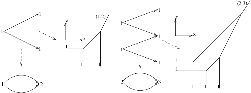
Figure 5. The tropical curve for Ti1+i2+i3+i4+i5T_{i_{1}+i_{2}+i_{3}+i_{4}+i_{5}}.

Refer to caption

Figure 6. From quivers to tropical curves for K⁡(2)K(2).

As for all tropical curves, we have the notion of multiplicity at a vertex MultV⁡hσ\operatorname{Mult}_{V}h_{\sigma}. We modify the notion of multiplicity using the quiver QQ as follows. A vertex V∈hσV\in h_{\sigma} corresponds to a pair of incoming dimension vectors dV,1,dV,2d_{V,1},d_{V,2} with μ⁡(dV,1)<μ⁡(dV,2)\mu(d_{V,1})<\mu(d_{V,2}). We set

MultQ,V⁡hσ=⟨dV,1,dV,2⟩.\operatorname{Mult}_{Q,V}h_{\sigma}=\langle d_{V,1},d_{V,2}\rangle. (2.75)

The global multiplicity is

MultQ⁡hσ=∏VMultQ,V⁡hσ.\operatorname{Mult}_{Q}h_{\sigma}=\prod_{V}\operatorname{Mult}_{Q,V}h_{\sigma}. (2.76)

To compare with the usual notion of tropical multiplicity, notice that in fact

MultV⁡hσ=1m​|⟨d¯V,1,d¯V,2⟩|\operatorname{Mult}_{V}h_{\sigma}=\frac{1}{m}|\langle\overline{d}_{V,1},\overline{d}_{V,2}\rangle| (2.77)

(we still write ⟨⋅,⋅⟩\langle\cdot,\,\cdot\rangle for the product of the reduced dimension vectors, computed on K⁡(m)K(m)).
Example. In the example of subquivers Q1,Q2⊂K^​(2)Q_{1},Q_{2}\subset\widehat{K}(2) of section 2.3 we have

MultQ1⁡hTi1+i2+i3=Mult⁡hTi1+i2+i3=1,\operatorname{Mult}_{Q_{1}}h_{T_{i_{1}+i_{2}+i_{3}}}=\operatorname{Mult}h_{T_{i_{1}+i_{2}+i_{3}}}=1,

and also

MultQ2⁡hTi1+i2+i3+i4+i5=Mult⁡hTi1+i2+i3+i4+i5=1.\operatorname{Mult}_{Q_{2}}h_{T_{i_{1}+i_{2}+i_{3}+i_{4}+i_{5}}}=\operatorname{Mult}h_{T_{i_{1}+i_{2}+i_{3}+i_{4}+i_{5}}}=1.

But we can compute

MultQ2⁡hTi1+i2+i4+i5=1,Mult⁡hTi1+i2+i4+i5=2.\operatorname{Mult}_{Q_{2}}h_{T_{i_{1}+i_{2}+i_{4}+i_{5}}}=1,\operatorname{Mult}h_{T_{i_{1}+i_{2}+i_{4}+i_{5}}}=2.

Finally, we will denote by 𝒮Q\mathcal{S}_{Q} the (finite) set of all rational tropical curves hσh_{\sigma} that we constructed for σ∈𝔖∞\sigma\in\mathfrak{S}^{\infty}, and by 𝒮Q​(μ)⊂𝒮Q\mathcal{S}_{Q}(\mu)\subset\mathcal{S}_{Q} the subset of curves whose outgoing dimension vector has prescribed slope, namely μ​(dout​(h))=μ\mu(d_{\operatorname{out}}(h))=\mu.

We now move on the the general case, working over the base rings of section 2.5. Recall in this case we have the additional parameter k≥1k\geq 1. We fix (2k−1)​s(2^{k}-1)s vertical lines, (2k−1)​S(2^{k}-1)S horizontal lines in ℝ2\mathbb{R}^{2} generically. We label the vertical lines 𝔡ij,I\mathfrak{d}_{i_{j},I} with elements of {i1,…,is}×{I⊂{1,…,k},I≠∅}\{i_{1},\dots,i_{s}\}\times\{I\subset\{1,\dots,k\},I\neq\emptyset\} in lexicographic order, starting from the rightmost line. Similarly we label the vertical lines 𝔡ij,J\mathfrak{d}_{i_{j},J} with elements of {is+1,…,iS}×{J⊂{1,…,k},J≠∅}\{i_{s+1},\dots,i_{S}\}\times\{J\subset\{1,\dots,k\},J\neq\emptyset\} in lexicographic order, starting from the lowest line. In other words, the set of all lines 𝔡ij,I\mathfrak{d}_{i_{j},I} is labelled with {i1,…,is+S}×{I⊂{1,…,k},I≠∅}\{i_{1},\dots,i_{s+S}\}\times\{I\subset\{1,\dots,k\},I\neq\emptyset\} in clockwise order starting from the rightmost vertical line, 𝔡i1,{1}\mathfrak{d}_{i_{1},\{1\}} to the top horizontal line, 𝔡is+S,{1,…,k}\mathfrak{d}_{i_{s+S},\{1,\dots,k\}}.
Example. The simplest case of a subquiver i2→i1i_{2}\to i_{1} with k=2k=2 is shown in Figure 7.

Refer to caption

Figure 7. Line arrangement with k=2k=2.

Pick σ∈𝔖∞\sigma\in\mathfrak{S}^{\infty}. We want to construct a tropical curve hσh_{\sigma} from σ\sigma. If σ\sigma first appears in 𝔖0\mathfrak{S}^{0} then σ=Tip,I\sigma=T_{i_{p},I} for some vertex ipi_{p} and I⊂{1,…,k}I\subset\{1,\dots,k\}. Then we are in a degenerate case and we just choose hσh_{\sigma} to be the corresponding line 𝔡ip,I\mathfrak{d}_{i_{p},I}. If σ\sigma first appears in 𝔖1\mathfrak{S}^{1} and Parents⁡(σ)={Tip,I,Tiq,J}\operatorname{Parents}(\sigma)=\{T_{i_{p},I},T_{i_{q},J}\} with p<qp<q then 1≤p≤s1\leq p\leq s and s+1≤q≤Ss+1\leq q\leq S. We define hσh_{\sigma} as the unique tropical curve hσ:Γσ→ℝ2h_{\sigma}\!:\Gamma_{\sigma}\to\mathbb{R}^{2} with unbounded vertical edge 𝔡ip,I\mathfrak{d}_{i_{p},I} and unbounded horizontal edge 𝔡iq,J\mathfrak{d}_{i_{q},J}. Then for σ∈𝔖i\sigma\in\mathfrak{S}^{i} with i>1i>1, we construct hσh_{\sigma} inductively precisely as in the discussion above, using now the weight (2.61) in the balancing condition (2.63). Similarly, we define the multiplicity of a vertex V∈hσV\in h_{\sigma} by (2.75), namely if the vertex arises from commuting xp↦xp​(1+c1​xr1​d1)⟨d1,p⟩x_{p}\mapsto x_{p}(1+c_{1}x^{r_{1}d_{1}})^{\langle d_{1},p\rangle} and xp↦(1+c2​xr2​d2)⟨d2,p⟩x_{p}\mapsto(1+c_{2}x^{r_{2}d_{2}})^{\langle d_{2},p\rangle} its multiplicity is ⟨r1​d1,r2​d2⟩\langle r_{1}d_{1},r_{2}d_{2}\rangle. The global multiplicity of hσh_{\sigma} is then given by (2.76).

As we mentioned in section 2.5, Assumption 4 in the definition of naive sorting diagrams does not hold in general for diagrams over R~k\widetilde{R}_{k}. Correction terms will arise from a class of disconnected tropical curves, i.e. maps from disconnected trees, which we now define. Fix any ordered ll-uple of elements of 𝔖k∞\mathfrak{S}^{\infty}_{k} with the same slope,

(σ1,…,σl)∈𝔖k∞,μ⁡(σi)=μ⁡(σi+1),(\sigma_{1},\dots,\sigma_{l})\in\mathfrak{S}^{\infty}_{k},\mu(\sigma_{i})=\mu(\sigma_{i+1}), (2.78)

such that σi≺σi+1\sigma_{i}\prec\sigma_{i+1} in 𝔖k∞\mathfrak{S}^{\infty}_{k}, and the sets I1,…​IlI_{1},\dots I_{l} underlying σ1,…,σl\sigma_{1},\dots,\sigma_{l} are pairwise disjoint. We define a tropical curve hσ1⋯σlh_{\sigma_{1}\cdots\sigma_{l}} simply as the union of the tropical curves hσ1,…,hσlh_{\sigma_{1}},\dots,h_{\sigma_{l}} (a map from the disjoint union ∪li=1Γσi\cup^{l}_{i=1}\Gamma_{\sigma_{i}}). We still use the notation Legs(hσ1⋯σl)\operatorname{Legs}(h_{\sigma_{1}\cdots\sigma_{l}}) for the set of lines 𝔡i,I\mathfrak{d}_{i,I} appearing in the image of hh.

To each curve hσ1⋯σlh_{\sigma_{1}\cdots\sigma_{l}} we attach inductively a weight function fσ1⋯σlf_{\sigma_{1}\cdots\sigma_{l}} as follows. We know from (2.59) that σ\sigma acts by xp↦xp​(1+c​uI​xr​d)⟨d,ip⟩x_{p}\mapsto x_{p}(1+cu_{I}x^{rd})^{\langle d,i_{p}\rangle} for some primitive dd. We set

fσ=cr​uI​xr​d.f_{\sigma}=\frac{c}{r}u_{I}x^{rd}. (2.79)

Suppose then inductively that fσ1⋯σl−1=αuIxr​df_{\sigma_{1}\cdots\sigma_{l-1}}=\alpha u_{I}x^{rd} for some primitive dd and α∈ℂ\alpha\in\mathbb{C}, and similarly fσl=α′​uI′​xr′​d′f_{\sigma_{l}}=\alpha^{\prime}u_{I^{\prime}}x^{r^{\prime}d^{\prime}}. Then we set

fσ1⋯σl=12⟨rd,r′d′⟩αα′uI∪I′xr​d+r′​d′.f_{\sigma_{1}\cdots\sigma_{l}}=\frac{1}{2}\langle rd,r^{\prime}d^{\prime}\rangle\alpha\,\alpha^{\prime}u_{I\cup I^{\prime}}x^{rd+r^{\prime}d^{\prime}}. (2.80)

Representing fσ1⋯σlf_{\sigma_{1}\cdots\sigma_{l}} in the form c​uI​xdcu_{I}x^{d}, we set

dout(hσ1⋯σl)=d.d_{\operatorname{out}}(h_{\sigma_{1}\cdots\sigma_{l}})=d. (2.81)

We extend the notion of multiplicity for hσ1⋯σlh_{\sigma_{1}\cdots\sigma_{l}} inductively as follows:

MultQ(hσ1⋯σl)=12MultQ(hσ1⋯σl−1)⟨dout(hσ1⋯σl−1),dout(σl)⟩.\operatorname{Mult}_{Q}(h_{\sigma_{1}\cdots\sigma_{l}})=\frac{1}{2}\operatorname{Mult}_{Q}(h_{\sigma_{1}\cdots\sigma_{l-1}})\langle d_{\operatorname{out}}(h_{\sigma_{1}\cdots\sigma_{l-1}}),d_{\operatorname{out}}(\sigma_{l})\rangle. (2.82)

We write 𝒮Q,k\mathcal{S}_{Q,k} for the set of all tropical curves hσ1⋯σlh_{\sigma_{1}\cdots\sigma_{l}} (we do not fix ll). For a fixed slope μ\mu, we write 𝒮Q,k​(μ)\mathcal{S}_{Q,k}(\mu) for the subset of 𝒮Q,k\mathcal{S}_{Q,k} given by all curves hσ1⋯σlh_{\sigma_{1}\cdots\sigma_{l}} with μ(dout(hσ1⋯σl))=μ\mu(d_{\operatorname{out}}(h_{\sigma_{1}\cdots\sigma_{l}}))=\mu.

Fix a curve hσ1⋯σl∈𝒮Q,kh_{\sigma_{1}\cdots\sigma_{l}}\in\mathcal{S}_{Q,k}. From this we find a unique weight vector

w=(w1,…,ws+S),\textbf{w}=(\textbf{w}_{1},\dots,\textbf{w}_{s+S}),
wq=(wq​1,…,wq​lq),\textbf{w}_{q}=(w_{q1},\dots,w_{ql_{q}}),

with 1≤wp​1≤⋯≤wq​lq1\leq w_{p1}\leq\dots\leq w_{ql_{q}}, and pairwise disjoint sets

Jq​j⊂{1,…,k},q=1,…,s+S;j=1,…,lq,J_{qj}\subset\{1,\dots,k\},q=1,\dots,s+S;\,j=1,\dots,l_{q},

with #​Jq​j=wq​j,\#J_{qj}=w_{qj}, such that

Legs(hσ1⋯σl)={𝔡iq,Jq​j|q=1,…,s+S;j=1,…,lq}.\operatorname{Legs}(h_{\sigma_{1}\cdots\sigma_{l}})=\{\mathfrak{d}_{i_{q},J_{qj}}|\,q=1,\dots,s+S;\,j=1,\dots,l_{q}\}.

Let us denote by NQ,ktrop​({Jq​j})N^{\operatorname{trop}}_{Q,k}(\{J_{qj}\}) the number of curves hσ1⋯σlh_{\sigma_{1}\cdots\sigma_{l}} giving rise to the same sets Jq​jJ_{qj}, counted with the multiplicity (2.82). By the construction of hσ1⋯σlh_{\sigma_{1}\cdots\sigma_{l}} in terms of sorting diagrams, it is clear that NQ,ktrop​({Jq​j})N^{\operatorname{trop}}_{Q,k}(\{J_{qj}\}) only depends on the vector w, not the actual subsets Jq​jJ_{qj}.

We denote this number by NQ,ktrop​(w)N^{\operatorname{trop}}_{Q,k}(\textbf{w}).

Notice that in fact dout=∑i|wi|​id_{\operatorname{out}}=\sum_{i}|\textbf{w}_{i}|\,i, so by abuse of notation we write μ⁡(w)\mu(\textbf{w}) and ⟨⋅,w⟩\langle\cdot,\textbf{w}\rangle for the slope μ⁡(dout)\mu(d_{\operatorname{out}}), respectively the linear form ⟨⋅,dout⟩\langle\cdot,d_{\operatorname{out}}\rangle. Similarly we will often write

xw=x∑i|wi|​i=x|w1|i1⋯x|ws+S|is+Sx^{\textbf{w}}=x^{\sum_{i}|\textbf{w}_{i}|\,i}=x^{|\textbf{w}_{1}|}_{i_{1}}\cdots x^{|\textbf{w}_{s+S}|}_{i_{s+S}} (2.83)

and

[w]=[∑i|wi|​i],[\,\textbf{w}\,]=[\,\sum_{i}|\textbf{w}_{i}|\,i\,], (2.84)

the equivalence class of the underlying dimension vector. For a fixed weight vector w we set

Rw=∏i=1s+S∏j=1l1(−1)wi​j−1wi​j2R_{\textbf{w}}=\prod^{s+S}_{i=1}\prod^{l_{1}}_{j=1}\frac{(-1)^{w_{ij}-1}}{w^{2}_{ij}} (2.85)

and

w¯=∑i|wi|​i¯=(∑i>s|wi|,∑i≤s|wi|).\overline{\textbf{w}}=\overline{\sum_{i}|\textbf{w}_{i}|\,i}=(\sum_{i>s}|\textbf{w}_{i}|,\sum_{i\leq s}|\textbf{w}_{i}|). (2.86)

3. Main results

Throughout this section we will concentrate on BB-framings for K⁡(m)K(m), and so on framings at sources on K~​(m)\widetilde{K}(m). The situation for FF-framings is completely analogous. We will use the notation (f​(x))​[xd](f(x))[x^{d}] to denote the coefficient of xdx^{d} in f⁡(x)f(x). We start in the simple situation described in sections 2.3, 2.4. According to Lemma 2.21 and Lemma 2.30, our main example is a finite subquiver Q⊂K~​(2)Q\subset\widetilde{K}(2) (although soon we will need to restrict to representations of slope μ≠12\mu\neq\frac{1}{2} in order to have Assumption 3 in place). The following lemma simply summarizes our simplified construction in sections 2.3, 2.4 and the first part of section 2.7.

Lemma 3.1.

Suppose that Assumptions 1, 2, 4 hold. Then there is a bijective correspondence between operators TdT_{d} with μ⁡(d)=μ\mu(d)=\mu appearing in the stable sorting diagram 𝔖∞\mathfrak{S}^{\infty} and tropical curves h∈𝒮Q​(μ)h\in\mathcal{S}_{Q}(\mu). Moreover

d=dout​(h)=∑𝔡i∈Legs⁡(h)i.d=d_{\operatorname{out}}(h)=\sum_{\mathfrak{d}_{i}\in\operatorname{Legs}(h)}i. (3.2)
Lemma 3.3.

Suppose that Assumptions 1-4 hold. Let Td1≺⋯≺TdrT_{d_{1}}\prec\dots\prec T_{d_{r}} be the maximal sequence of operators with μ⁡(di)=μ\mu(d_{i})=\mu appearing in 𝔖∞\mathfrak{S}^{\infty}. Then the composition Td1∘⋯∘TdrT_{d_{1}}\circ\cdots\circ T_{d_{r}} acts by

xp↦xp​∏h∈𝒮Q​(μ)(1+xdout​(h))⟨dout​(h),p⟩.x_{p}\mapsto x_{p}\prod_{h\in\mathcal{S}_{Q}(\mu)}(1+x^{d_{\operatorname{out}}(h)})^{\langle d_{\operatorname{out}}(h),p\rangle}. (3.4)
Proof.

We know that TdiT_{d_{i}} corresponds to a curve h∈𝒮Q​(μ⁡(di))h\in\mathcal{S}_{Q}(\mu(d_{i})) and di=dout​(h)d_{i}=d_{\operatorname{out}}(h), Tdi​(xp)=xp​(1+xdout​(h))⟨dout​(h),p⟩T_{d_{i}}(x_{p})=x_{p}(1+x^{d_{\operatorname{out}}(h)})^{\langle d_{\operatorname{out}}(h),p\rangle}. This correspondence is bijective, and operators of the same slope μ⁡(di)\mu(d_{i}) commute, and so compose simply as in the statement. ∎

Corollary 3.5.

Let Q⊂K^​(2)Q\subset\widehat{K}(2) be a subquiver with s+1s+1 sinks, ss sources. Then for 1≤p≤S1\leq p\leq S, μ≠12\mu\neq\frac{1}{2},

θQ,μ,is+p​(x)=∏h∈𝒮Q​(μ)(1+xdout​(h))⟨ip−ip−1+⋯±i1,dout​(h)⟩.\theta_{Q,\mu,i_{s+p}}(x)=\prod_{h\in\mathcal{S}_{Q}(\mu)}(1+x^{d_{\operatorname{out}}(h)})^{\langle i_{p}-i_{p-1}+\dots\pm i_{1},d_{\operatorname{out}}(h)\rangle}. (3.6)

In other words

χ⁡(ℳQs,is+p​(d))=∏h∈𝒮Q​(μ)(1+xdout​(h))⟨ip−ip−1+⋯±i1,dout​(h)⟩​[xd].\chi(\mathcal{M}^{s,i_{s+p}}_{Q}(d))=\prod_{h\in\mathcal{S}_{Q}(\mu)}(1+x^{d_{\operatorname{out}}(h)})^{\langle i_{p}-i_{p-1}+\dots\pm i_{1},d_{\operatorname{out}}(h)\rangle}[x^{d}]. (3.7)
Proof.

First by Reineke’s Theorem 2.11 (and our choice of a minimal labelling) we know

θQ,μ​(xi1)=xi1​(θQ,μ,is+1​(x))−1.\theta_{Q,\mu}(x_{i_{1}})=x_{i_{1}}(\theta_{Q,\mu,i_{s+1}}(x))^{-1}. (3.8)

By Lemma 3.3 we have

θQ,μ​(xi1)=xi1​∏h∈𝒮Q​(μ)(1+xdout​(h))⟨dout​(h),i1⟩,\theta_{Q,\mu}(x_{i_{1}})=x_{i_{1}}\prod_{h\in\mathcal{S}_{Q}(\mu)}(1+x^{d_{\operatorname{out}}(h)})^{\langle d_{\operatorname{out}}(h),i_{1}\rangle}, (3.9)

from which of course we find

θQ,μ,is+1​(x)=∏h∈𝒮Q​(μ)(1+xdout​(h))⟨i1,dout​(h)⟩.\theta_{Q,\mu,i_{s+1}}(x)=\prod_{h\in\mathcal{S}_{Q}(\mu)}(1+x^{d_{\operatorname{out}}(h)})^{\langle i_{1},d_{\operatorname{out}}(h)\rangle}. (3.10)

This establishes (3.6) for p=1p=1. For p>1p>1 we have again by Reineke’s Theorem

θQ,μ​(xip+1)=xip+1​(θQ,μ,is+p​(x))−1​(θQ,μ,is+p+1​(x))−1.\theta_{Q,\mu}(x_{i_{p+1}})=x_{i_{p+1}}(\theta_{Q,\mu,i_{s+p}}(x))^{-1}(\theta_{Q,\mu,i_{s+p+1}}(x))^{-1}. (3.11)

Therefore

θQ,μ,is+p+1​(x)=xip+1​(θQ,μ​(xip+1))−1​(θQ,μ,is+p​(x))−1.\theta_{Q,\mu,i_{s+p+1}}(x)=x_{i_{p+1}}(\theta_{Q,\mu}(x_{i_{p+1}}))^{-1}(\theta_{Q,\mu,i_{s+p}}(x))^{-1}. (3.12)

By Lemma 3.3 we have

(θQ,μ​(xip+1))−1=1xip+1​∏h∈𝒮Q​(μ)(1+xdout​(h))⟨ip+1,dout​(h)⟩.(\theta_{Q,\mu}(x_{i_{p+1}}))^{-1}=\frac{1}{x_{i_{p+1}}}\prod_{h\in\mathcal{S}_{Q}(\mu)}(1+x^{d_{\operatorname{out}}(h)})^{\langle i_{p+1},d_{\operatorname{out}}(h)\rangle}. (3.13)

and assuming by induction that (3.6) holds for (θQ,μ,is+p​(x))−1(\theta_{Q,\mu,i_{s+p}}(x))^{-1} we find

θQ,μ,is+p+1​(x)\displaystyle\theta_{Q,\mu,i_{s+p+1}}(x) =∏h∈𝒮Q​(μ)(1+xdout​(h))⟨ip+1,dout​(h)⟩​∏h∈𝒮Q​(μ)(1+xdout​(h))⟨−ip+⋯±i1,dout​(h)⟩\displaystyle=\prod_{h\in\mathcal{S}_{Q}(\mu)}(1+x^{d_{\operatorname{out}}(h)})^{\langle i_{p+1},d_{\operatorname{out}}(h)\rangle}\prod_{h\in\mathcal{S}_{Q}(\mu)}(1+x^{d_{\operatorname{out}}(h)})^{\langle-i_{p}+\dots\pm i_{1},d_{\operatorname{out}}(h)\rangle}
=∏h∈𝒮Q​(μ)(1+xdout​(h))⟨ip+1−ip+⋯±i1,dout​(h)⟩.\displaystyle=\prod_{h\in\mathcal{S}_{Q}(\mu)}(1+x^{d_{\operatorname{out}}(h)})^{\langle i_{p+1}-i_{p}+\dots\pm i_{1},d_{\operatorname{out}}(h)\rangle}. (3.14)

∎

Corollary 3.15.

Let d¯\overline{d} be a fixed dimension vector for K⁡(2)K(2). Choose Q⊂K^​(2)Q\subset\widehat{K}(2) with s+1s+1 sinks, ss sources for ss large enough (depending on d¯\overline{d}). Then

χ⁡(ℳK⁡(2)s,B​(d¯))=∑[d]∼d¯∑p=1s∏h∈𝒮Q​(μ)(1+xdout​(h))⟨ip−ip−1+⋯±i1,dout​(h)⟩​[xd],\chi(\mathcal{M}^{s,B}_{K(2)}(\overline{d}))=\sum_{[d]\sim\overline{d}}\sum^{s}_{p=1}\prod_{h\in\mathcal{S}_{Q}(\mu)}(1+x^{d_{\operatorname{out}}(h)})^{\langle i_{p}-i_{p-1}+\dots\pm i_{1},d_{\operatorname{out}}(h)\rangle}[x^{d}], (3.16)

where the first sum is over all equivalence classes [d][d] of dimension vectors supported on QQ and compatible with d¯\overline{d}.

Proof.

This is an immediate consequence of Weist’s theorem in the form (2.3) and the result we just proved, since the cardinality of the support of d∈ℕ​K^​(2)0d\in\mathbb{N}\widehat{K}(2)_{0} compatible with d¯\overline{d} is uniformly bounded (and so dd can be moved to an equivalent dimension vector in a large enough quiver QQ of the type we want). ∎

Refer to caption

Figure 8. Curves contributing to χ⁡(ℳK⁡(2)s,B​(4,6))\chi(\mathcal{M}^{s,B}_{K(2)}(4,6)).

Example. By (2.24) we know B2,3​(x,y)=(1+x2​y3)2B_{2,3}(x,y)=(1+x^{2}y^{3})^{2}, so χ⁡(ℳK⁡(2)s,B)​(4,6)=1\chi(\mathcal{M}^{s,B}_{K(2)})(4,6)=1. This is witnessed already by a subquiver Q⊂K^​(2)Q\subset\widehat{K}(2) with s=4s=4, S=3S=3. A lengthy but elementary computation shows that 𝒮Q​(25)\mathcal{S}_{Q}(\frac{2}{5}) contains only two curves h′,h′′h^{\prime},h^{\prime\prime} with Legs⁡(h′)={𝔡i1,𝔡i2,𝔡i3,𝔡i5,𝔡i6}\operatorname{Legs}(h^{\prime})=\{\mathfrak{d}_{i_{1}},\mathfrak{d}_{i_{2}},\mathfrak{d}_{i_{3}},\mathfrak{d}_{i_{5}},\mathfrak{d}_{i_{6}}\} and Legs⁡(h′′)={𝔡i2,𝔡i3,𝔡i4,𝔡i6,𝔡i7}\operatorname{Legs}(h^{\prime\prime})=\{\mathfrak{d}_{i_{2}},\mathfrak{d}_{i_{3}},\mathfrak{d}_{i_{4}},\mathfrak{d}_{i_{6}},\mathfrak{d}_{i_{7}}\} (see Figure 8). So dout​(h′)=i1+i2+i3+i5+i6d_{\operatorname{out}}(h^{\prime})=i_{1}+i_{2}+i_{3}+i_{5}+i_{6} and dout​(h′′)=i2+i3+i4+i6+i7d_{\operatorname{out}}(h^{\prime\prime})=i_{2}+i_{3}+i_{4}+i_{6}+i_{7}, and

∏h∈𝒮Q​(25)(1+xdout​(h))⟨i2−i1,dout​(h)⟩=(1+xi1​xi2​xi3​xi5​xi6)​(1+xi2​xi3​xi4​xi6​xi7).\prod_{h\in\mathcal{S}_{Q}(\frac{2}{5})}(1+x^{d_{\operatorname{out}}(h)})^{\langle i_{2}-i_{1},d_{\operatorname{out}}(h)\rangle}=(1+x_{i_{1}}x_{i_{2}}x_{i_{3}}x_{i_{5}}x_{i_{6}})(1+x_{i_{2}}x_{i_{3}}x_{i_{4}}x_{i_{6}}x_{i_{7}}). (3.17)

Expanding out we see a term xi1​xi22​xi32​xi5​xi62​x7x_{i_{1}}x^{2}_{i_{2}}x^{2}_{i_{3}}x_{i_{5}}x^{2}_{i_{6}}x_{7} corresponding to

χ⁡(ℳQs,i6​(i1+2​i2+2​i3+i5+2​i6+i7))=1,\chi(\mathcal{M}^{s,i_{6}}_{Q}(i_{1}+2i_{2}+2i_{3}+i_{5}+2i_{6}+i_{7}))=1, (3.18)

the unique contribution to χ⁡(ℳK⁡(2)s,B​(4,6))\chi(\mathcal{M}^{s,B}_{K(2)}(4,6)).

Let us now move on to the general case of the base rings R~k\widetilde{R}_{k}. We start with a result which says how to reconstruct the weight function fσ1⋯σlf_{\sigma_{1}\cdots\sigma_{l}} from the tropical curve hσ1⋯σlh_{\sigma_{1}\cdots\sigma_{l}}.

Lemma 3.19.

The weight function attached to the tropical curve h=hσ1⋯σlh=h_{\sigma_{1}\cdots\sigma_{l}} is given by

fσ1⋯σl=MultQ(h)∏i,J((−1)#​J−1#​J(#J−1)!∏l∈Jui​l)xdout​(h),f_{\sigma_{1}\cdots\sigma_{l}}=\operatorname{Mult}_{Q}(h)\prod_{i,J}\left(\frac{(-1)^{\#J-1}}{\#J}(\#J-1)!\prod_{l\in J}u_{il}\right)x^{d_{\operatorname{out}}(h)}, (3.20)

where the product is over all i∈Q0i\in Q_{0} and J⊂{1,…,k}J\subset\{1,\dots,k\} for which 𝔡i,J∈Legs⁡(h)\mathfrak{d}_{i,J}\in\operatorname{Legs}(h), and

dout​(h)=∑𝔡i,J∈Legs⁡(h)(#​J)​i.d_{\operatorname{out}}(h)=\sum_{\mathfrak{d}_{i,J}\in\operatorname{Legs}(h)}(\#J)i. (3.21)
Proof.

Suppose first that l=1l=1, so h=hσh=h_{\sigma} for some σ∈𝔖∞\sigma\in\mathfrak{S}^{\infty}. If σ\sigma first appears in 𝔖k0\mathfrak{S}^{0}_{k}, then hσh_{\sigma} is just one of the lines 𝔡i,J\mathfrak{d}_{i,J}, we have MultQ⁡(hσ)=1\operatorname{Mult}_{Q}(h_{\sigma})=1 since there are no trivalent vertices at all, and dout=(#​J)​id_{\operatorname{out}}=(\#J)i, Ind⁡(dout)=#​J\operatorname{Ind}(d_{\operatorname{out}})=\#J. Thus (3.20) holds by the definition of the operators Ti,JT_{i,J}, (2.45), and of fσf_{\sigma}, 2.79. Suppose now that σ\sigma first appears in 𝔖i,k\mathfrak{S}^{i},k with i≥1i\geq 1, and Parents⁡(σ)={σ1,σ2}\operatorname{Parents}(\sigma)=\{\sigma_{1},\sigma_{2}\}. Then by induction and Lemma 2.47 we see that

fσ\displaystyle f_{\sigma} =MultQ⁡(hσ1)​MultQ⁡(hσ2)\displaystyle=\operatorname{Mult}_{Q}(h_{\sigma_{1}})\operatorname{Mult}_{Q}(h_{\sigma_{2}})
⋅⟨d1,out,d2,out⟩​∏i,J((−1)#​J−1#​J​(#​J−1)!​∏l∈Jui​l)​xd1,out+d2,out,\displaystyle\cdot\langle d_{1,\operatorname{out}},d_{2,\operatorname{out}}\rangle\prod_{i,J}\left(\frac{(-1)^{\#J-1}}{\#J}(\#J-1)!\prod_{l\in J}u_{il}\right)x^{d_{1,\operatorname{out}}+d_{2,\operatorname{out}}}, (3.22)

where the product is over all i∈Q0i\in Q_{0} and J⊂{1,…,k}J\subset\{1,\dots,k\} for which 𝔡i,J∈Legs⁡(hσ1)∪Legs⁡(hσ2)\mathfrak{d}_{i,J}\in\operatorname{Legs}(h_{\sigma_{1}})\cup\operatorname{Legs}(h_{\sigma_{2}}). Notice that Legs⁡(hσ1)∩Legs⁡(hσ2)=∅\operatorname{Legs}(h_{\sigma_{1}})\cap\operatorname{Legs}(h_{\sigma_{2}})=\emptyset and Legs⁡(hσ1)∪Legs⁡(hσ2)=Legs⁡(hσ)\operatorname{Legs}(h_{\sigma_{1}})\cup\operatorname{Legs}(h_{\sigma_{2}})=\operatorname{Legs}(h_{\sigma}). It is then clear by induction that

dout=d1,out+d2,out=∑𝔡i,J∈Legs⁡(h)(#​J)​i.d_{\operatorname{out}}=d_{1,\operatorname{out}}+d_{2,\operatorname{out}}=\sum_{\mathfrak{d}_{i,J}\in\operatorname{Legs}(h)}(\#J)i. (3.23)

On the other hand

MultQ⁡(hσ1)​MultQ⁡(hσ2)​⟨d1,out,d2,out⟩=MultQ⁡(hσ)\operatorname{Mult}_{Q}(h_{\sigma_{1}})\operatorname{Mult}_{Q}(h_{\sigma_{2}})\langle d_{1,\operatorname{out}},d_{2,\operatorname{out}}\rangle=\operatorname{Mult}_{Q}(h_{\sigma}) (3.24)

by the definition of multiplicity (2.76).

For general hσ1⋯σlh_{\sigma_{1}\cdots\sigma_{l}} the same argument works, this time by induction on ll. ∎

Lemma 3.25.

Let σ1≺⋯≺σr\sigma_{1}\prec\dots\prec\sigma_{r} be the maximal sequence of operators with slope μ\mu in 𝔖k∞\mathfrak{S}^{\infty}_{k}. Then the product σ1∘⋯∘σr\sigma_{1}\circ\cdots\circ\sigma_{r} acts by

xp↦xp⋅fp,x_{p}\mapsto x_{p}\cdot f_{p}, (3.26)

where

log⁡fp=∑h∈𝒮Q,k​(μ)⟨dout​(h),ip⟩​fh.\log f_{p}=\sum_{h\in\mathcal{S}_{Q,k}(\mu)}\langle d_{\operatorname{out}}(h),i_{p}\rangle f_{h}. (3.27)
Proof.

As in the proof of Lemma 2.47 we write σi\sigma_{i} as the exponential of some derivation in the noncommutaive Poisson algebra, exp⁡({σ~i,⋅})\exp(\{\widetilde{\sigma}_{i},\cdot\}). Retaining only the first order corrections, the Baker-Campbell-Hausdorff formula tells us that log∏iexp({σ~i,⋅})\log\prod_{i}\exp(\{\widetilde{\sigma}_{i},\cdot\}) is a sum of terms of the form

{12​{…​12​{12​{σ~j1,σ~j2},σ~j3},…,σ~jl},⋅}\{\frac{1}{2}\{\dots\frac{1}{2}\{\frac{1}{2}\{\widetilde{\sigma}_{j_{1}},\widetilde{\sigma}_{j_{2}}\},\widetilde{\sigma}_{j_{3}}\},\dots,\widetilde{\sigma}_{j_{l}}\},\cdot\} (3.28)

for l≥1l\geq 1 and 1≤j1<j2<⋯<jl1\leq j_{1}<j_{2}<\cdots<j_{l}. However the formula (2.53) in the proof of Lemma 2.47 tells us that this is an exact computation, i.e. only first order corrections actually happen. And again by (2.53) and the definition of weight function (2.80), we have

12{…12{12{σ~j1,σ~j2},σ~j3},…,σ~jl}=fσj1⋯σjl.\frac{1}{2}\{\dots\frac{1}{2}\{\frac{1}{2}\{\widetilde{\sigma}_{j_{1}},\widetilde{\sigma}_{j_{2}}\},\widetilde{\sigma}_{j_{3}}\},\dots,\widetilde{\sigma}_{j_{l}}\}=f_{\sigma_{j_{1}}\cdots\sigma_{j_{l}}}. (3.29)

In other words there is a one to one correspondence between correction terms in the Baker-Campbell-Hausdorff formula and weight functions of (possibly disconnected) curves in 𝒮Q,k​(μ)\mathcal{S}_{Q,k}(\mu). ∎

We will express ff in terms of our numbers NQ,ktropN^{\operatorname{trop}}_{Q,k}. This computation should be compared with [GPS] Theorem 2.8 (although our case is simpler).

Lemma 3.30.

The function fpf_{p} in (3.27) can be written as

fp(tx)=∑w:μ⁡(w)=μ⟨w,ip⟩Rw|Aut⁡(w)|NQ,ktrop(w)(tx)w.f_{p}(tx)=\sum_{\emph{\textbf{w}}:\mu(\emph{\textbf{w}})=\mu}\langle\emph{\textbf{w}},i_{p}\rangle\frac{R_{\emph{\textbf{w}}}}{|\operatorname{Aut}(\emph{\textbf{w}})|}N^{\operatorname{trop}}_{Q,k}(\emph{\textbf{w}})\,(tx)^{\emph{\textbf{w}}}. (3.31)
Proof.

For a fixed curve h∈𝒮Q,k​(μ)h\in\mathcal{S}_{Q,k}(\mu) we find a weight vector w and sets Jq​jJ_{qj} as in section 2.7. We can rewrite (3.20) in terms of w as

fh=MultQ⁡(h)​∏q=1s+S∏j=1lq((−1)wq​j−1wq​j​(wq​j−1)!​∏r∈Jq​juq​r)​xw.f_{h}=\operatorname{Mult}_{Q}(h)\prod^{s+S}_{q=1}\prod^{l_{q}}_{j=1}\left(\frac{(-1)^{w_{qj}-1}}{w_{qj}}(w_{qj}-1)!\prod_{r\in J_{qj}}u_{qr}\right)\,x^{\textbf{w}}. (3.32)

Summing over all curves hh which give rise to the same weight vector w and the same sets Jq​jJ_{qj} we find a contribution to log⁡fp\log f_{p} given by

⟨w,ip⟩​NQ,ktrop​(w)​∏q=1s+S∏j=1lq((−1)wq​j−1wq​j​(wq​j−1)!​∏r∈Jq​juq​r)​xw.\langle\textbf{w},i_{p}\rangle N^{\textrm{trop}}_{Q,k}(\textbf{w})\prod^{s+S}_{q=1}\prod^{l_{q}}_{j=1}\left(\frac{(-1)^{w_{qj}-1}}{w_{qj}}(w_{qj}-1)!\prod_{r\in J_{qj}}u_{qr}\right)\,x^{\textbf{w}}. (3.33)

Summing up over all Jq​jJ_{qj} would then give

⟨w,ip⟩​NQ,ktrop​(w)​∏q=1s+S∏j=1lq(−1)wq​j−1wq​j2​tw​xw,\langle\textbf{w},i_{p}\rangle N^{\operatorname{trop}}_{Q,k}(\textbf{w})\prod^{s+S}_{q=1}\prod^{l_{q}}_{j=1}\frac{(-1)^{w_{qj}-1}}{w^{2}_{qj}}\,t^{\textbf{w}}x^{\textbf{w}},

but one can show that this overcounts curves by a factor |Aut⁡(w)||\operatorname{Aut}(\textbf{w})|.

∎

Theorem 3.34.

Let ipi_{p} (for some 1≤p≤s1\leq p\leq s) be a sink of QQ with precisely one source mapping to it, say ip¯i_{\bar{p}} (s+1≤p¯≤s+Ss+1\leq\bar{p}\leq s+S). Then

logθQ,μ,p¯(tx)≡∑w:μ⁡(w)=μ⟨ip,w⟩Rw|Aut⁡(w)|NQ,ktrop(w)(tx)wmod(t1k+1,…,ts+Sk+1).\log\theta_{Q,\mu,\bar{p}}(tx)\equiv\sum_{\emph{\textbf{w}}:\mu(\emph{\textbf{w}})=\mu}\langle i_{p},\emph{\textbf{w}}\rangle\frac{R_{\emph{\textbf{w}}}}{|\operatorname{Aut}(\emph{\textbf{w}})|}N^{\operatorname{trop}}_{Q,k}(\emph{\textbf{w}})\,(tx)^{\emph{\textbf{w}}}\mod(t^{k+1}_{1},\dots,t^{k+1}_{s+S}). (3.35)
Proof.

Reineke’s theorem 2.11 gives

θμ​(xp)=xp⋅(θQ,μ,p¯​(t​x))−1.\theta_{\mu}(x_{p})=x_{p}\cdot(\theta_{Q,\mu,\bar{p}}(tx))^{-1}. (3.36)

We also know

θμ​(xp)≡xp​fp​(1+ρ),ρ∈(t1k+1,…,ts+Sk+1)\theta_{\mu}(x_{p})\equiv x_{p}\,f_{p}\,(1+\rho),\,\rho\in(t^{k+1}_{1},\dots,t^{k+1}_{s+S}) (3.37)

where fpf_{p} is given by 3.27. Therefore

log⁡θQ,μ,p¯​(t​x)\displaystyle\log\theta_{Q,\mu,\bar{p}}(tx) ≡−log⁡fpmod(t1k+1,…,ts+Sk+1)\displaystyle\equiv-\log f_{p}\mod(t^{k+1}_{1},\dots,t^{k+1}_{s+S})
=∑w:μ⁡(w)=μ⟨ip,w⟩Rw|Aut⁡(w)|NQ,ktrop(w)(tx)w.\displaystyle=\sum_{\textbf{w}:\mu(\textbf{w})=\mu}\langle i_{p},\textbf{w}\rangle\frac{R_{\textbf{w}}}{|\operatorname{Aut}(\textbf{w})|}N^{\operatorname{trop}}_{Q,k}(\textbf{w})\,(tx)^{\textbf{w}}.

∎

We say that a vertex i∈Q0i\in Q_{0} is a boundary vertex (i∈∂Qi\in\partial Q) if it is has valency 11 in the undirected graph underlying QQ. By making QQ larger if necessary, we can assume that the only boundary vertices of QQ are sinks. The result we just proved tells us how to compute θQ,μ,p​(t​x)\theta_{Q,\mu,p}(tx) (to all orders) for all sources p∈Q0p\in Q_{0} mapping to a boundary sink, in terms of certain tropical curves. Using the special feature that QQ sits in a tree (since the connected components of K~​(m)\widetilde{K}(m) are infinite directed mm-regular trees), we can propagate this calculation to an arbitrary sink of QQ.

Theorem 3.38.

Let Q⊂K~​(m)Q\subset\widetilde{K}(m) be a finite connected subquiver, with only sinks as boundary vertices. Then for each source i∈Q0i\in Q_{0}, there exist distinct sinks ip​qi^{pq} with 1≤p≤P1\leq p\leq P, 1≤q≤(m−1)p−11\leq q\leq(m-1)^{p-1} such that

logθQ,μ,i(x)≡∑w:μ⁡(w)=μ⟨ε(i),w⟩Rw|Aut⁡(w)|NQ,ktrop(w)(tx)wmod(t1k+1,…,ts+Sk+1),\log\theta_{Q,\mu,i}(x)\equiv\sum_{\emph{\textbf{w}}:\mu(\emph{\textbf{w}})=\mu}\langle\varepsilon(i),\emph{\textbf{w}}\rangle\frac{R_{\emph{\textbf{w}}}}{|\operatorname{Aut}(\emph{\textbf{w}})|}N^{\operatorname{trop}}_{Q,k}(\emph{\textbf{w}})\,(tx)^{\emph{\textbf{w}}}\mod(t^{k+1}_{1},\dots,t^{k+1}_{s+S}), (3.39)

with

ε⁡(i)=i11−(i21+…​i2​(m−1))+⋯±(iP​1+⋯+iP​(m−1)P−1).\varepsilon(i)=i^{11}-(i^{21}+\dots i^{2(m-1)})+\dots\pm(i^{P1}+\dots+i^{P(m-1)^{P-1}}). (3.40)
Proof.

Let us define recursively subsets Xn,n≥1X_{n},n\geq 1 of the set of sources of QQ, by

X1\displaystyle X_{1} ={i is a source, i→j∈∂Q},\displaystyle=\{i\text{ is a source, }i\to j\in\partial Q\},
Xn\displaystyle X_{n} ={i is a source, i→j∣ for all sources i′≠i with i′→j,i′∈Xn−1}∪Xn−1.\displaystyle=\{i\text{ is a source, }i\to j\mid\text{ for all sources }i^{\prime}\neq i\text{ with }i^{\prime}\to j,i^{\prime}\in X_{n-1}\}\cup X_{n-1}.

Recall that we denoted by SS the number of sources. We claim that the set XSX_{S} contains all the sources in QQ. Arguing by contradiction, let i0i_{0} be a source which is not contained in XSX_{S}. By the definition of XSX_{S}, we can pick any sink j0j_{0} with i→j0i\to j_{0}, and find a source i1≠ii_{1}\neq i with i1→j0i_{1}\to j_{0} and i1∉XS−1i_{1}\notin X_{S-1}. Notice that i1i_{1} must map to a sink j1≠j0j_{1}\neq j_{0}, otherwise i1i_{1} would be a boundary vertex. Then in turn by the definition of XS−1X_{S-1} we can find a source i2≠i1i_{2}\neq i_{1} with i2→j1i_{2}\to j_{1} and i2∉XS−2i_{2}\notin X_{S-2}. We must have i2≠i0i_{2}\neq i_{0} too otherwise QQ would contain an (unoriented) cycle. Proceeding by induction, given in∉XS−ni_{n}\notin X_{S-n} (with n<S−1n<S-1) this maps to a sink jn≠jn−1j_{n}\neq j_{n-1} (otherwise ini_{n} would lie on the boundary), and in fact jnj_{n} is also distinct from all j0,j1,…​jn−2j_{0},j_{1},\ldots j_{n-2} (otherwise QQ would contain an unoriented cycle); then by definition of XS−nX_{S-n} we find in+1≠ini_{n+1}\neq i_{n} with in+1→jni_{n+1}\to j_{n} and in≠XS−n−1i_{n}\neq X_{S-n-1}, in+1i_{n+1} also distinct from all i0,i1,…​in−1i_{0},i_{1},\ldots i_{n-1} (no cycles). We stop on reaching a source iS−1i_{S-1}. Thus we find a sequence of distinct sources i0,i1,…​iS−1i_{0},i_{1},\ldots i_{S-1}, with in∉XS−ni_{n}\notin X_{S-n}. In particular, this would say all the sources in QQ do not lie in X1X_{1}, which is clearly impossible. This proves the claim.

For a source ii, we define d⁡(i,∂Q)d(i,\partial Q) to be the least nn such that i∈Xni\in X_{n}. We will prove our statement by induction on d⁡(i,∂Q)d(i,\partial Q). If d⁡(i,∂Q)=1d(i,\partial Q)=1 it reduces to Theorem 3.34. Suppose now the statement is known for all sources j∈Q0j\in Q_{0} with d⁡(i,∂Q)≤Pd(i,\partial Q)\leq P and choose i∈Q0i\in Q_{0} with d⁡(i,∂Q)=P+1d(i,\partial Q)=P+1. Then by the definition of distance ii maps to a sink i11i^{11} such that all other sources j1,…,jm−1j_{1},\dots,j_{m-1} mapping to i11i^{11} (except ii) satisfy d⁡(jq,∂Q)≤Pd(j_{q},\partial Q)\leq P. We apply Reineke’s Theorem to i11i^{11}, finding

θQ,μ​(xi11)=xi11​(θQ,μ,i​(t​x))−1​∏q=1m−1(θQ,μ,jq​(t​x))−1.\theta_{Q,\mu}(x_{i^{11}})=x_{i^{11}}(\theta_{Q,\mu,i}(tx))^{-1}\prod^{m-1}_{q=1}(\theta_{Q,\mu,j_{q}}(tx))^{-1}. (3.41)

By our previous results,

θQ,μ​(xi11)=xi11​fi11,\theta_{Q,\mu}(x_{i^{11}})=x_{i^{11}}f_{i^{11}}, (3.42)

with

fi11=∑w:μ⁡(w)=μ⟨w,i11⟩Rw|Aut⁡(w)|NQ,ktrop(w)(tx)w.f_{i^{11}}=\sum_{\textbf{w}:\mu(\textbf{w})=\mu}\langle\textbf{w},i^{11}\rangle\frac{R_{\textbf{w}}}{|\operatorname{Aut}(\textbf{w})|}N^{\operatorname{trop}}_{Q,k}(\textbf{w})\,(tx)^{\textbf{w}}. (3.43)

By induction,

logθQ,μ,jq(tx)≡∑w:μ⁡(w)=μ⟨ε(jq),w⟩Rw|Aut⁡(w)|NQ,ktrop(w)(tx)wmod(t1k+1,…,ts+Sk+1)\log\theta_{Q,\mu,j_{q}}(tx)\equiv\sum_{\textbf{w}:\mu(\textbf{w})=\mu}\langle\varepsilon(j_{q}),\textbf{w}\rangle\frac{R_{\textbf{w}}}{|\operatorname{Aut}(\textbf{w})|}N^{\operatorname{trop}}_{Q,k}(\textbf{w})\,(tx)^{\textbf{w}}\mod(t^{k+1}_{1},\dots,t^{k+1}_{s+S}) (3.44)

with

ε⁡(jq)=jq11−(jq21+⋯+jq2​(m−1))+⋯±(jqP​1+⋯+jqP​(m−1)P−1).\varepsilon(j_{q})=j^{11}_{q}-(j^{21}_{q}+\dots+j^{2(m-1)}_{q})+\dots\pm(j^{P1}_{q}+\dots+j^{P(m-1)^{P-1}}_{q}). (3.45)

Therefore

log⁡θQ,μ,i​(t​x)\displaystyle\log\theta_{Q,\mu,i}(tx) ≡−log⁡fi11−log⁡θQ,μ,j1​(t​x)−⋯−log⁡θQ,μ,jm−1​(t​x)\displaystyle\equiv-\log f_{i^{11}}-\log\theta_{Q,\mu,j_{1}}(tx)-\dots-\log\theta_{Q,\mu,j_{m-1}}(tx) (3.46)
≡∑w:μ⁡(w)=μ⟨ε(i),w⟩Rw|Aut⁡(w)|NQ,ktrop(w)(tx)w\displaystyle\equiv\sum_{\textbf{w}:\mu(\textbf{w})=\mu}\langle\varepsilon(i),\textbf{w}\rangle\frac{R_{\textbf{w}}}{|\operatorname{Aut}(\textbf{w})|}N^{\operatorname{trop}}_{Q,k}(\textbf{w})\,(tx)^{\textbf{w}} (3.47)

with

ε⁡(i)=i11−(j111+⋯+jm−111)\displaystyle\varepsilon(i)=i^{11}-(j^{11}_{1}+\dots+j^{11}_{m-1})
+(j121+⋯+jm−121+⋯+j122+⋯+jm−122+⋯+j12​(m−1)+⋯+jm−12​(m−1))\displaystyle+(j^{21}_{1}+\dots+j^{21}_{m-1}+\dots+j^{22}_{1}+\dots+j^{22}_{m-1}+\dots+j^{2(m-1)}_{1}+\dots+j^{2(m-1)}_{m-1})
±(j1P​1+⋯+jm−1P​1+⋯+j1P​2+⋯+jm−1P​2+⋯+j1P​(m−1)P−1+⋯+jm−1P​(m−1)P−1)\displaystyle\pm(j^{P1}_{1}+\dots+j^{P1}_{m-1}+\dots+j^{P2}_{1}+\dots+j^{P2}_{m-1}+\dots+j^{P(m-1)^{P-1}}_{1}+\dots+j^{P(m-1)^{P-1}}_{m-1}) (3.48)

where equivalence is modulo (t1k+1,…,ts+Sk+1)(t^{k+1}_{1},\dots,t^{k+1}_{s+S}) as usual. ∎

Then Weist’s Theorem yields the following.

Corollary 3.49.

Let d¯\overline{d} be a fixed dimension vector for K⁡(m)K(m). Choose Q⊂K~​(m)Q\subset\widetilde{K}(m) large enough and k≫1k\gg 1 (depending on d¯\overline{d}). Then

χ(ℳK⁡(m)s,B(d¯))=∑[d]∼d¯∑p=s+1s+Sexp(∑w:μ⁡(w)=μ⟨ε(ip),w⟩Rw|Aut⁡(w)|NQ,ktrop(w)(tx)w)[(tx)d]\chi(\mathcal{M}^{s,B}_{K(m)}(\overline{d}))=\sum_{[d]\sim\overline{d}}\sum^{s+S}_{p=s+1}\exp\left(\sum_{\emph{\textbf{w}}:\mu(\emph{\textbf{w}})=\mu}\langle\varepsilon(i_{p}),\emph{\textbf{w}}\rangle\frac{R_{\emph{\textbf{w}}}}{|\operatorname{Aut}(\emph{\textbf{w}})|}N^{\operatorname{trop}}_{Q,k}(\emph{\textbf{w}})\,(tx)^{\emph{\textbf{w}}}\right)[(tx)^{d}] (3.50)

where the first sum is over all equivalence classes [d][d] of dimension vectors supported on QQ and compatible with d¯\overline{d}.

Finally, with these results in place, the GW/Kronecker correspondence gives back a comparison between the genuine tropical invariants Ntrop​(w′)N^{\operatorname{trop}}(\textbf{w}^{\prime}) of [GPS] and our ad hoc counts NQtrop​(w)N^{\operatorname{trop}}_{Q}(\textbf{w}), at least in a special case. Indeed by the Kronecker/GW correspondence 1.1, we have

χ⁡(ℳK⁡(m)s,B​(h​a,h​b))=exp⁡(am​∑r≥1∑|Pa|=r​a,|Pb|=r​br​Na,b​[(Pa,Pb)]​x(r​a,r​b))​[x(h​a,h​b)].\chi(\mathcal{M}^{s,B}_{K(m)}(ha,hb))=\exp\left(\frac{a}{m}\sum_{r\geq 1}\sum_{|P_{a}|=ra,|P_{b}|=rb}rN_{a,b}[(P_{a},P_{b})]x^{(ra,rb)}\right)[x^{(ha,hb)}]. (3.51)

By Theorem 2.74, the right hand side can be rewritten as

exp⁡(am​∑r≥1∑|Pa|=r​a,|Pb|=r​b∑w′∼(Pa,Pb)R(Pa,Pb)|w′|Aut⁡(w′)|​Ntrop​(w′)​r​x(r​a,r​b))​[x(h​a,h​b)].\exp\left(\frac{a}{m}\sum_{r\geq 1}\sum_{|P_{a}|=ra,|P_{b}|=rb}\sum_{\textbf{w}^{\prime}\sim(P_{a},P_{b})}\frac{R_{(P_{a},P_{b})|\textbf{w}^{\prime}}}{|\operatorname{Aut}(\textbf{w}^{\prime})|}N^{\operatorname{trop}}(\textbf{w}^{\prime})rx^{(ra,rb)}\right)[x^{(ha,hb)}]. (3.52)

On the other hand for QQ and kk large enough the Euler characteristic can also be computed as

∑[d]∼(h​a,h​b)∑p=s+1s+Sexp(∑w:μ⁡(w)=aa+b⟨ε(ip),w⟩Rw|Aut⁡(w)|NQ,ktrop(w)(tx)w)[(tx)d].\sum_{[d]\sim(ha,hb)}\sum^{s+S}_{p=s+1}\exp\left(\sum_{\textbf{w}:\mu(\textbf{w})=\frac{a}{a+b}}\langle\varepsilon(i_{p}),\textbf{w}\rangle\frac{R_{\textbf{w}}}{|\operatorname{Aut}(\textbf{w})|}N^{\operatorname{trop}}_{Q,k}(\textbf{w})(tx)^{\textbf{w}}\right)[(tx)^{d}]. (3.53)

Suppose now that h=1h=1. Since the vector (a,b)(a,b) is primitive, we must have the equality

am∑|Pa|=a,|Pb|=b∑w′∼(Pa,Pb)\displaystyle\frac{a}{m}\sum_{|P_{a}|=a,|P_{b}|=b}\sum_{\textbf{w}^{\prime}\sim(P_{a},P_{b})} R(Pa,Pb)|w′|Aut⁡(w′)|​Ntrop​(w′)\displaystyle\frac{R_{(P_{a},P_{b})|\textbf{w}^{\prime}}}{|\operatorname{Aut}(\textbf{w}^{\prime})|}N^{\operatorname{trop}}(\textbf{w}^{\prime})
=∑p=s+1s+S∑[w]∼(a,b)⟨ε⁡(ip),w⟩​Rw|Aut⁡(w)|​NQ,ktrop​(w).\displaystyle=\sum^{s+S}_{p=s+1}\sum_{[\,\textbf{w}\,]\sim(a,b)}\langle\varepsilon(i_{p}),\textbf{w}\rangle\frac{R_{\textbf{w}}}{|\operatorname{Aut}(\textbf{w})|}N^{\operatorname{trop}}_{Q,k}(\textbf{w}). (3.54)

We do not know a direct proof of this equality, although we believe that one exists which exploits the comparison between the multiplicities MultQ,V⁡h\operatorname{Mult}_{Q,V}h and MultV⁡h\operatorname{Mult}_{V}h as in (2.75) and (2.77).

4. Connection with quiver gauge theories

We will briefly explain the physical interpretation of K⁡(m)K(m) and how this picture (especially the paper of F. Denef [De]) gives a possible motivation for the constructions we have presented. Unfortunately the author is not an expert in the area, so our account will be very naive and imprecise. The reader should consult [De].

Let S1,S2S_{1},S_{2} be two Lagrangian 33-spheres in a compact Calabi-Yau threefold XX, meeting transversely and positively in mm points, so for the intersection product (the DSZ product in this context) we have ⟨[S1],[S2]⟩=m\langle[S_{1}],[S_{2}]\rangle=m. In the terminology of [De] Section 3.1 S1,S2S_{1},S_{2} are parton D3-branes. The generalised Kronecker quiver K⁡(m)K(m) with dimension vector d=(d1,d2)d=(d_{1},d_{2}) arises in the study of the string theory on spacetime compactified on XX with mm open strings with boundaries on one of d1d_{1} D-branes of type [S1][S_{1}] and one of d2d_{2} D-branes of type [S2][S_{2}].

The fundamental parameter in this theory is the string coupling constant gsg_{s}. For positive gs≈0g_{s}\approx 0, and when the D-branes have small but nonvanishing phase difference and spacetime separation, the theory becomes a quiver quantum mechanics modelled on K⁡(m)K(m). In particular the Witten index of the theory can be computed as χ​(ℳK⁡(m)​(d))\chi(\mathcal{M}_{K(m)}(d)).

A very different picture emerges for large coupling constant gsg_{s}. In this regime the BPS states for the theory become multi-centered, molecule-like configurations of d1d_{1} “monopoles” with charge Q and d2d_{2} “electrons” with charge q, with DSZ product ⟨Q,q⟩=m\langle\textbf{Q},\textbf{q}\rangle=m (i.e. the “monopoles” have magnetic charge mm, the “electrons” have electric charge 11). What Weist’s Theorem 2.1 says in this regime is that we can compute the same Witten index by summing over all multi-centered BPS configurations with charges Q1,…,Qℓ1\textbf{Q}_{1},\dots,\textbf{Q}_{\ell_{1}} and q1,…,qℓ2\textbf{q}_{1},\dots,\textbf{q}_{\ell_{2}} such that the DSZ product ⟨Qi,qj⟩\langle\textbf{Q}_{i},\textbf{q}_{j}\rangle is at most 11 for i=1​…,ℓ1,j=1,…,ℓ2i=1\,\dots,\ell_{1},j=1,\dots,\ell_{2} (i.e. such that each pair of interacting particles looks like a simple monopole-electron system, corresponding to K⁡(1)K(1)). The K~​(m)\widetilde{K}(m) constraint in this regime means that the splitting into charges Qi,qj\textbf{Q}_{i},\textbf{q}_{j} must be compatible with the original DSZ product ⟨Q,q⟩=m\langle\textbf{Q},\textbf{q}\rangle=m.

For each of these multi-centered configurations, going back to gs≈0g_{s}\approx 0 will give theories based on configurations of partons, with the same total Witten index. In other words one can compute the total Witten index by summing up over all the ways of splitting the boundary conditions for the open strings. Notice that so far we have ignored the framing, but this could easily be introduced by adding an additional parton D-brane SS to the discussion above.
Remark. The large gsg_{s} viewpoint gives an interesting interpretation of Weist’s gluing result [We] Corollary 5.28. Mathematically, in its simplest form, this says that if we have two representations R′,R′′R^{\prime},R^{\prime\prime} of K~​(m)\widetilde{K}(m) with dimension vectors d′,d′′d^{\prime},d^{\prime\prime} and ⟨d′,d′′⟩=1\langle d^{\prime},d^{\prime\prime}\rangle=1 we can glue them by identifying two sinks j′∈R0′,j′′∈R0′′j^{\prime}\in R^{\prime}_{0},j^{\prime\prime}\in R^{\prime\prime}_{0}. The new dimension vector is d=d′+d′′d=d^{\prime}+d^{\prime\prime}. Now from the gs≫0g_{s}\gg 0 perspective we are simply superimposing our two special multi-centered configurations at two “electrons”. Weist’s gluing corresponds to the statement that the total configuration we obtain is BPS, as long as the two multi-centered configurations behave mutually like a simple monopole-electron system,

⟨∑iQi′+∑jqj′,∑iQi′′+∑jqj′′⟩=1.\langle\sum_{i}\textbf{Q}^{\prime}_{i}+\sum_{j}\textbf{q}^{\prime}_{j},\sum_{i}\textbf{Q}^{\prime\prime}_{i}+\sum_{j}\textbf{q}^{\prime\prime}_{j}\rangle=1.

What we wish to retain from this physical picture is that passing to the universal cover for quiver representations corresponds to splitting either boundary conditions (i.e. D-branes, partons) for small gsg_{s} or particles (for large gsg_{s}) into a number of constituents. Then we can recover χ\chi by summing up over all configurations of all possible types. The advantage of this physical point of view is that it suggests an analogy between Weist’s Theorem (2.3) and Theorem 2.74, i.e. in both cases we are computing our invariants (Witten indexes) by summing up over all boundary conditions (in other words it allows us to regard [d~][\,\tilde{d}\,] as specifying boundary conditions for open strings, while w specifies “boundary conditions”, really legs, for tropical curves).

Finally we should mention that the special case m=2m=2 (with framing) has a physical interpretation as a certain S​U​(2)SU(2) Seiberg-Witten theory, as discussed in [GMN] Section 2.2. The Kontsevich-Soibelman wall-crossing has been interpreted in the context of Seiberg-Witten theories by Gaiotto, Moore and Nietzke [GMN]. In the special case m=2m=2 the relevant identity is (using Kontsevich-Soibelman operators on K⁡(2)K(2))

T1,0∘T0,1=T0,1∘T1,2∘T2,3⋯T−21,1⋯T3,2∘T2,1∘T1,0T_{1,0}\circ T_{0,1}=T_{0,1}\circ T_{1,2}\circ T_{2,3}\cdots T^{-2}_{1,1}\cdots T_{3,2}\circ T_{2,1}\circ T_{1,0}

which they interpret as going from strong coupling (the left hand side) to weak coupling (the right hand side). In Corollary 3.15 we have seen which curves carry a contribution to the operator which represents one of the states of charge (a,a+1)(a,a+1).

References

  • [De] F. Denef, Quantum quivers and Hall/hole halos, J. High Energy Phys. 2002, no. 10, 023, 42 pp.
  • [ER] J. Engel and M. Reineke, Smooth models of quiver moduli, Math. Z. 262 (2009), no. 4, 817–848.
  • [GMN] D. Gaiotto, G. Moore and A. Nietzke, Four dimensional wall-crossing via three-dimensional field theory, Comm. Math. Phys. 299 (2010), no. 1, 163-224.
  • [GP] M. Gross and R. Pandharipande, Quivers, curves, and the tropical vertex, Port. Math. 67 (2010), no. 2, 211�259.
  • [GPS] M. Gross, R. Pandharipande and B. Siebert, The tropical vertex, Duke Math. J. 153 (2010), no. 2, 297�362.
  • [KS] M. Kontsevich and Y. Soibelman, Stability structures, motivic Donaldson-Thomas invariants and cluster transformations, arXiv:0811.2435.
  • [Re] M. Reineke, Poisson automorphisms and quiver moduli, J. Inst. Math. Jussieu 9 (2010), no. 3, 653�667.
  • [We] T. Weist, Localization in quiver moduli spaces, arXiv:0903.5442.