Instantaneous interquark potential in generalized Landau gauge in SU(3) lattice QCD: a possible gauge for the quark potential model

The Landau gauge is one of the most popular gauges in QCD, and its gauge fixing is given by

where $A_{\mu}(x)\equiv A_{\mu}^{a}(x)T^{a}\in\mathfrak{su}(N_{c})$ are gluon fields, with $\mathfrak{su}(N_{c})$ generator $T^{a}(a=1,2,\dots N_{c}^{2}-1)$. The Landau gauge keeps the Lorentz covariance and the global SU($N_{c}$) color symmetry. These symmetries simplify the tensor structure of various quantities in QCD. For example, the gluon propagator $D_{\mu\nu}^{ab}(p)$ is simply expressed as

due to the symmetries and the transverse property. Owing to this advanced feature, the Landau gauge is often used both in the Schwinger-Dyson formalism [16, 17] and in lattice QCD studies for quarks and gluons [18, 19].

In Euclidean QCD, the Landau gauge has a global definition to minimize the global quantity,

by the gauge transformation. This global definition is more strict, and the local form in Eq.(1) can be obtained from the minimization of $R_{\rm L}$. Since the quantity $R_{\rm L}$ physically means the total amount of gauge-field fluctuations, and therefore the Landau gauge maximally suppresses artificial gauge-field fluctuations originated from the gauge degrees of freedom.

Here, we comment on non-locality of the gauge fields. Through the gauge fixing procedure, gauge fields have non-locality stemming from the Faddeev-Popov determinant. In the Landau gauge, this non-locality of gauge fields is Lorentz covariant.

Using the Landau gauge, or a covariant and globally symmetric gauge, the color confinement has been mathematically investigated in terms of the BRST charge and the inverse Higgs theorem, which is known as the “Kugo-Ojima criterion” [8].

The Coulomb gauge is also a popular gauge in QCD, and its gauge fixing is given by

This condition resembles the Landau gauge condition (Eq.(1)), but there are no constraints on $A_{0}$. In the Coulomb gauge, the Lorentz covariance is partially broken, and gauge field components are completely decoupled into two parts, $\vec{A}$ and $A_{0}$: $\vec{A}$ behave as canonical variables and $A_{0}$ becomes an instantaneous potential.

Similarly in the Landau gauge, the Coulomb gauge has a global definition to minimize the global quantity

by the gauge transformation. Note here that the Euclidean metric is not necessary for the global definition of the Coulomb gauge. Note also that there appears no nonlocality in the temporal direction in the Coulomb gauge. Due to this feature, a hadron mass measurement can be safely performed using a spatially-extended quark source in the Coulomb gauge in lattice QCD calculations [20].

In the Coulomb gauge, one of the advantages is the compatibility with the canonical quantization [21]. The QCD Hamiltonian is expressed as

where $\rho^{a}$ is the color charge density, $\vec{E}^{a}$ and $\vec{B}^{a}$ are the color electric and magnetic field, respectively. Here, $K^{ab}(x,y)$ is the instantaneous Coulomb propagator [11] defined as

with the Faddeev-Popov operator

The confinement picture in the Coulomb gauge focuses on the Coulomb energy including the inverse of $M$. Here, the Coulomb energy is the non-local second term of the QCD Hamiltonian (6), and is regarded as the instantaneous potential. Near the Gribov horizon, where the Faddeev-Popov operator $M$ has zero eigenvalues [9], the Coulomb energy at large quark distance is expected to be largely enhanced and leads to a confining interquark potential, which is called as the “Gribov-Zwanziger scenario” [9, 10].

As Zwanziger showed, the Coulomb energy (instantaneous potential) $V_{\rm Coul}(R)$ in the Coulomb gauge gives an upper bound on the static interquark potential $V_{\rm phys}(R)$ [22], i.e.,

This inequality indicates that if the physical interquark potential is confining then the Coulomb energy $V_{\rm Coul}$ is also confining. Actually, lattice QCD calculations [11] show that the Coulomb energy (the instantaneous potential) between a quark and an antiquark leads to a linear potential, which characterizes the confinement. However, the slope of the instantaneous potential is too large, i.e., $2\sim 3$ times larger than the physical string tension, and this Coulomb system turns out to be an excited state.

As for the ground-state of the quark-antiquark system, Thorn and Greensite proposed the “gluon-chain picture” in the Coulomb gauge [13]. In fact, to screen the large Coulomb energy between the quark and the antiquark, chain-like gluons are dynamically generated between them. This gluon-chain is expected to give the linear potential between quarks. In other words, QCD string can be regarded as a “chain” of gluons in the Coulomb gauge.

We investigate the instantaneous potential $V_{\lambda}(R)$ defined by Eq.(23) in generalized Landau gauge. Figure 1 shows lattice QCD results of $V_{\lambda}(R)$ for typical values of $\lambda$. In this figure, the statistic error is small and the error bars are hidden in the symbols.

In the Coulomb gauge ($\lambda=0$), the instantaneous potential shows linear behavior, while there is no linear part at all in the Landau gauge ($\lambda=1$). Thus, there is a large gap between these gauges in terms of the instantaneous potential. In our framework, however, these two gauges are connected continuously.

By varying the $\lambda$-parameter from 1 to 0 in the generalized Landau gauge, we find that the instantaneous potential $V_{\lambda}(R)$ changes continuously, and the infrared slope of the potential $V_{\lambda}(R)$ at $R\simeq 0.8{\rm fm}$ grows monotonically, from the Landau gauge to the Coulomb gauge, as shown in Fig. 1. Note here that the growing of the infrared slope of $V_{\lambda}(R)$ is quite rapid for $\lambda\lesssim 0.1$, near the Coulomb gauge, while the infrared slope is rather small and almost unchanged for $\lambda=0.1\sim 1$.

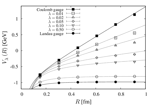
To analyze the instantaneous potential $V_{\lambda}(R)$ quantitatively, we fit the lattice QCD results using the Coulomb plus linear Ansatz as

where $A_{\lambda}$ is the Coulomb coefficient and $C_{\lambda}$ a constant. Here, $\sigma_{\lambda}$ is the infrared slope of the potential, which we call as “instantaneous string tension”. Besides the Coulomb plus linear Ansatz, we try several candidates of the functional form, $-A/R+\sigma(1-e^{-\varepsilon R})/\varepsilon$, $-A\exp(-mR)/R$, $-A/R+\sigma R^{d}$, and $-A/R^{d}$ apart from an irrelevant constant, but they are less workable. The curves in Fig. 1 are the best-fit results using Eq.(25). The Coulomb plus linear Ansatz works well at least for $R\lesssim 0.8$fm, which is relevant region for hadron physics. We note that the Yukawa form of $-Ae^{-mR}/R$ also works well near the Landau gauge, which will be discussed in relation to the gluon-propagator behavior in Sec.VI-C.

We summarize the best-fit parameters and the fit-range in Table 1. While the Coulomb coefficient $A_{\lambda}$ has a relatively weak $\lambda$-dependence, the instantaneous string tension $\sigma_{\lambda}$ shows a strong $\lambda$-dependence near the Coulomb gauge, i.e., $\lambda\lesssim 0.1$.

We comment on the asymptotic value of the instantaneous potential $\sigma_{\lambda}$. In the deep IR limit, $R\rightarrow\infty$, $V_{\lambda}(R)$ goes to a saturated value, except for $\lambda=0$. This feature is closely related to the property of the temporal link-variable correlator $\langle\mathrm{Tr}\{U_{4}^{\dagger}(x)U_{4}(y)\}\rangle$, as will be discussed in Sec.VI.

Now, we focus on the $\lambda$-dependence of instantaneous string tension $\sigma_{\lambda}$ in Fig. 2. For $0.1\lesssim\lambda\leq 1$, including the Landau gauge ($\lambda$=1), $\sigma_{\lambda}$ is almost zero, so that this region can be regarded as “Landau-like.” For $\lambda\lesssim 0.1$, $V_{\lambda}(R)$ is drastically changed near the Coulomb gauge, and $\sigma_{\lambda}$ grows rapidly in this small region. Finally, in the Coulomb gauge ($\lambda$=0), one finds $\sigma_{\lambda}\simeq 2.6\sigma_{\rm phys}$, with $\sigma_{\rm phys}\simeq 0.89$GeV/fm.

Note that the instantaneous string tension $\sigma_{\lambda}$ continuously changes from $0$ to $(2\sim 3)\sigma_{\rm phys}$, according to the change from the Landau gauge to the Coulomb gauge, and therefore there exists some specific $\lambda$-parameter of $\lambda_{C}\in[0,1]$ where the slope of the instantaneous potential $V_{\lambda}(R)$ coincides with the physical string tension $\sigma_{\rm phys}$. Since the instantaneous potential generally depends on the lattice parameter $\beta$, i.e., the lattice spacing $a$ [11, 7], the value of $\lambda_{C}$ is $\beta$-dependence, although its dependence would be rather weak, as will be discussed in Sec.VI. However, from the continuity between the overconfining potential in the Coulomb gauge and the saturated potential in the Landau gauge, there must exist $\lambda_{C}\in[0,1]$ where the instantaneous string tension $\sigma_{\lambda}$ coincides with $\sigma_{\rm phys}$ for each lattice spacing. We call this specific gauge as “$\lambda_{C}$-gauge”. From Fig.2, the value of $\lambda_{C}$ is estimated to be about 0.02 at $\beta$=5.8. Note here that $\lambda_{C}\simeq 0.02\ll 1$ is very small, and then the $\lambda_{C}$-gauge is close to the Coulomb gauge, which indicates the small temporal non-locality.

Figure 3 shows the instantaneous potential $V_{\lambda}(R)$ at $\lambda=0.02\simeq\lambda_{C}$ and the physical static interquark potential $V_{\rm phys}(R)$. In this $\lambda_{C}$-gauge, $V_{\rm phys}(R)$ is found to be approximately reproduced by $V_{\lambda_{C}}(R)$ for $R\lesssim$ 0.8fm. While the physical static potential $V_{\rm phys}(R)$ is derived from the large-T behavior of the Wilson loop $W(R,T)$ [27] as

only instantaneous corerlation of the temporal link-variable $U_{4}$ approximately reproduces $V_{\rm phys}(R)$ in the $\lambda_{C}$-gauge, i.e.,

as is schematically illustrated in Fig.4.

On the relation to the confinement, which is a gauge independent phenomenon, the role of gluons generally depends on the choice of gauges, and the physical picture of the confinement would be changed according to gauges. For example, in the Coulomb gauge, the instantaneous Coulomb energy gives an overconfining potential, and the ground-state of the quark-antiquark system is described as the gluon-chain state. On the other hand, in the Landau gauge, the instantaneous potential has no linear part, and the ghost behavior in the deep-infrared region would be more important for the confinement.

In the $\lambda_{C}$-gauge, the physical interquark potential $V_{\rm phys}(R)$ is approximately reproduced by the instantaneous potential $V_{\lambda_{C}}(R)$. This physically means that all other complicated effects including dynamical gluons and ghosts are approximately cancelled in the $\lambda_{C}$-gauge, and therefore we do not need to introduce any redundant gluonic degrees of freedom. The absence of dynamical gluon degrees of freedom would be a desired property for the quark model picture.

In the previous subsection, we investigated the instantaneous potential $V_{\lambda}(R)$, which is defined by the Polyakov-line correlator with a minimum length on the lattice. For the quark-potential model, it is desired that the interquark potential does not have large dependence on the temporal length $T$ of the typical reaction scale. From this viewpoint, we investigate the “finite-time potential” $V_{\lambda}(R,T)$ defined by Eq.(18) in Sec.IV, and its temporal-length dependence. Here, $V_{\lambda}(R,T)$ is expressed by $T$-length terminated Polyakov-line $L(\vec{x},T)$ in Eq.(19), and a generalization of the instantaneous potential $V_{\lambda}(R)$.

First, we consider the Coulomb gauge [11, 7]. Figure 5 shows the lattice QCD result for $V_{\lambda}(R,T)$ in the Coulomb gauge. Similar to the instantaneous potential, $V_{\lambda}(R,T)$ is well reproduced by the Coulomb plus linear form. However, the parameter values are changed according to $T$-length. In particular, the slope of the potential becomes smaller as $T$ becomes larger, which shows an “instability” of $V_{\lambda}(R,T)$ in terms of $T$ in the Coulomb gauge.

For general $\lambda$, finite-time potential $V_{\lambda}(R,T)$ is found to be reproduced by the Coulomb plus linear form as

at least for $R\lesssim 0.8$fm, similarly for the instantaneous potential.

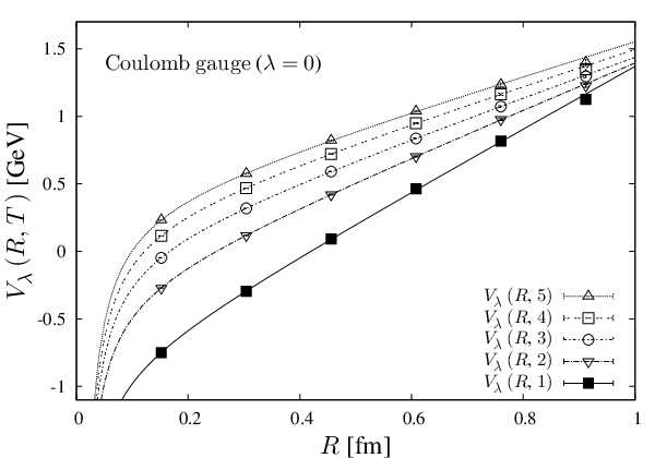
Since our main interest is linear part of the potential, we focus on “finite-time string tension” $\sigma_{\lambda}(T)$, the slope of $V_{\lambda}(R,T)$. Figure 6 shows $\sigma_{\lambda}(T)$ in generalized Landau gauge for typical values of $\lambda$. In Table 2, we summarize the best-fit parameters of $\sigma_{\lambda}(T)$ at $T=1,2,\dots,6$, and the ratio of $\sigma_{\lambda}(1)/\sigma_{\lambda}(6)$, $\sigma_{\lambda}(1)/\sigma_{\rm phys}$, and $\sigma_{\lambda}(6)/\sigma_{\rm phys}$, respectively.

On the $T$-dependence of the finite-time string tension $\sigma_{\lambda}(T)$, there are three groups of the $\lambda$-parameter region: (i) Coulomb-like region ($0\leq\lambda\ll\lambda_{C}$), (ii) Landau-like region ($\lambda_{C}\ll\lambda\leq 1$), and (iii) $\lambda_{C}$-like region ($\lambda\sim\lambda_{C}$).

(i) The first category is the Coulomb-like region of $0\leq\lambda\ll\lambda_{C}$, i.e., $0\leq\lambda\lesssim 0.01$. In this region, the instantaneous string tension $\sigma_{\lambda}\equiv\sigma_{\lambda}(T=1)$ is larger than the physical string tension $\sigma_{\rm phys}$, and the instantaneous potential $V_{\lambda}(R)\equiv V_{\lambda}(R,T=1)$ gives an overconfining potential. The ground-state of the quark-antiquark system is considered as the gluon-chain state. As the temporal length $T$ of the Polyakov-line increases, finite-time string tension $\sigma_{\lambda}(T)$ decreases and approaches to the physical string tension $\sigma_{\rm phys}$. This decreasing behavior is interpreted that the component of the ground-state, i.e., the gluon-chain state, becomes dominant as $T$-length becomes large. Thus, this region would not be compatible with the quark potential picture, because of the large $T$-dependence of the confining force $\sigma_{\lambda}(T)$ in addition to the dynamical generation of the gluon-chain.

(ii) The second category is the Landau-like region of $\lambda_{C}\ll\lambda\leq 1$, i.e. $0.1\lesssim\lambda\leq 1$. In this region, the instantaneous string tension is almost zero, i.e., $\sigma_{\lambda}\simeq 0$, and finite-time string tension $\sigma_{\lambda}(T)$ is an increasing function of $T$. Although its asymptotic value is unclear for $T\sim 0.8$ fm, $\sigma_{\lambda}(T)$ seems to approach to the physical string tension $\sigma_{\rm phys}$, which will be discussed in Sec.VI.

(iii) The third category is the $\lambda_{C}$-like region of $\lambda\sim\lambda_{C}$, i.e., $0.01\lesssim\lambda\lesssim 0.1$. In this region, the instantaneous string tension $\sigma_{\lambda}$ is approximately equal to the physical string tension, i.e., $\sigma_{\lambda}\simeq\sigma_{\rm phys}(\simeq$ 0.89GeV/fm), and the instantaneous potential $V_{\lambda}(R)$ approximately reproduces the physical static potential $V_{\rm phys}(R)$, as shown in Fig. 3. As the temporal length $T$ increases, finite-time string tension $\sigma_{\lambda}(T)$ is slightly changed and takes a little larger value ($\simeq$ 1.1GeV/fm) around $T\simeq$ 0.8fm. In particular, near $\lambda_{C}\simeq 0.02$, $\sigma_{\lambda}(T)$ shows only a weak $T$-dependence, while $\sigma_{\lambda}(T)$ largely changes as $T$ in the Coulomb gauge. As a whole, finite-time potential $V_{\lambda}(R,T)$ has small $T$-dependence, as shown in Fig. 7. This is also a desired feature for the linkage to the quark potential model.

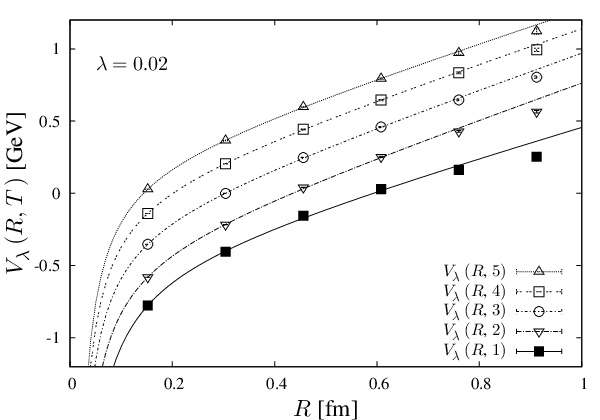
When the length $T$ of the Polyakov-line increases, $\lambda$-dependence of $\sigma_{\lambda}(T)$ is weakened, and $\sigma_{\lambda}(T)$ seems to converge to the physical string tension $\sigma_{\rm phys}$ for enough large $T$, as indicated in Fig.6.

There are two ingredients on the above gauge-dependence ($\lambda$-dependence): one is the large excess of the Coulomb energy in the Coulomb gauge, the other is the non-locality from the Faddeev-Popov determinant. From the fixing condition of generalized Landau gauge in Eq.(10), one finds that the $\lambda$-parameter controls the non-locality in the temporal direction. In the Landau gauge, the non-locality appears equally in spatial and temporal directions, while temporal non-locality disappears in the Coulomb gauge. If the Coulomb-energy excess can be neglected, e.g., for large $\lambda$, $V_{\lambda}(R,T)$ is expected to reproduce the static potential $V_{\rm phys}(R)$, when $T$-length and $R$ are large enough to neglect the non-locality scale. Owing to the $\lambda$-dependence of the non-locality, such a $T$-length exceeding the non-locality is to be larger for larger $\lambda$ in the Landau-like region.

Near the $\lambda_{C}$-gauge, finite-time potential $V_{\lambda}(R,T)$ has only weak $T$-length dependence. In other words, this can be regarded as an approximate “fixed point” against $T$ around $\lambda_{C}\simeq 0.02$. We conjecture that this is due to the approximate cancellation between the Coulomb-energy excess and the non-locality. Actually, in contrast to the large $T$-dependence of $V_{\lambda}(R,T)$ in the Coulomb gauge as shown in Fig.5, $V_{\lambda_{C}}(R,T)$ is rather stable against $T$-length in the $\lambda_{C}$-gauge, as shown in Fig.7.

First, we investigate the spatial correlator $G_{\lambda}(R)$ of the temporal link-variable $U_{4}$, and the relation to the instantaneous potential $V_{\lambda}(R)\equiv-\frac{1}{a}{\rm ln}G_{\lambda}(R)$. For the large spatial separation of $R\equiv|\vec{x}-\vec{y}|\rightarrow\infty$, $G_{\lambda}(R)$ behaves asymptotically as

where $\langle(U_{4})_{ij}\rangle=\frac{1}{3}\langle\mathrm{Tr}\ U_{4}\rangle\delta_{ij}\in\mathbf{R}$ from the global color symmetry. Here, $\frac{1}{3}\langle\mathrm{Tr}\ U_{4}\rangle^{2}$ is found to give the lower bound of $G_{\lambda}(R)$. If $\langle\mathrm{Tr}\ U_{4}\rangle$ takes some finite value, $V_{\lambda}(R)$ inevitably saturates for large $R$. Then, $\langle\mathrm{Tr}\ U_{4}\rangle=0$ is a necessary condition for the deep-infrared confinement feature of $V_{\lambda}(R=\infty)=\infty$.

In the Coulomb gauge, $\langle\mathrm{Tr}\ U_{4}\rangle$ is zero due to the remnant symmetry, as is shown in Appendix. Therefore, as $R\rightarrow\infty$, the correlator $G_{\lambda}(R)$ converges to zero, and $V_{\lambda}(R)\equiv-\frac{1}{a}{\rm ln}G_{\lambda}(R)\rightarrow+\infty$, which corresponds to the deep-infrared confinement.

For the general case of $\lambda\neq 0$, however, $\langle\mathrm{Tr}\ U_{4}\rangle$ has a non-zero value, and $G_{\lambda}(R)$ approaches to some finite constant. The finiteness of $\langle\mathrm{Tr}\ U_{4}\rangle$ gives a saturation of $V_{\lambda}(R)$, which leads to the absence of its linear part in the case of rapid convergence.

Figure 8 shows $G_{\lambda}(R)$ and its asymptotic value $\frac{1}{3}\langle\mathrm{Tr}\ U_{4}\rangle^{2}$ in the Landau and the Coulomb gauges. In the Landau gauge, $\langle\mathrm{Tr}\ U_{4}\rangle$ has a large expectation value, according to the maximization of $\sum_{x}\mathrm{Re}\ \mathrm{Tr}\ U_{\mu}(x)$, and $G_{\lambda}(R)$ rapidly converges to a finite constant for $R\gtrsim$ 0.4fm, which leads to a rapid saturation of the instantaneous potential $V_{\lambda}(R)$. In the Coulomb gauge, we find $\langle\mathrm{Tr}\ U_{4}\rangle=0$, and $G_{\lambda}(R)$ decreases monotonically to zero as $R$, which leads to $V_{\lambda}(R)=+\infty$ for $R=\infty$.

Figure 9 shows $\lambda$-dependence of $\frac{1}{3}\langle\mathrm{Tr}\ U_{4}\rangle$ in generalized Landau gauge. For $\lambda\neq 0$, $\langle\mathrm{Tr}\ U_{4}\rangle$ takes a non-zero real value, and it approaches to zero continuously as $\lambda\rightarrow 0$. Here, it largely changes in the small region of $0\leq\lambda\lesssim 0.1$. The finiteness of $\langle\mathrm{Tr}\ U_{4}\rangle$ is directly related to the infrared damping of the correlator $G_{\lambda}(R)$ and the infrared form of the instantaneous potential $V_{\lambda}(R)$.

Next, we consider $T$-length terminated Polyakov-line correlator $G_{\lambda}(R,T)$, which behaves asymptotically as

for large separation of $R=|\vec{x}-\vec{y}|$. As well as the instantaneous potential, $\frac{1}{3}\langle\mathrm{Tr}\ L(T)\rangle^{2}$ is found to give the lower bound of the correlator $G_{\lambda}(R,T)$, and the finiteness of $\langle\mathrm{Tr}\ L(T)\rangle$ is responsible for the infrared saturation of the finite-time potential $V_{\lambda}(R,T)$.

Figure 10 shows $T$-dependence of the terminated Polyakov-line $\frac{1}{3}\langle\mathrm{Tr}\ L(T)\rangle$ in generalized Landau gauge for typical values of $\lambda$. In the Coulomb gauge ($\lambda$=0), $\langle\mathrm{Tr}\ L(T)\rangle$ is always zero as well as $\langle\mathrm{Tr}\ U_{4}\rangle$, which means that $V_{\lambda}(R=\infty,T)=-\frac{1}{T}{\rm ln}G_{\lambda}(R=\infty,T)=+\infty$ for any values of $T$. Actually, finite-time potential $V_{\lambda}(R,T)$ always has a linear part in the Coulomb gauge, as shown in Fig.5.

For $\lambda\neq 0$, $\langle\mathrm{Tr}\ L(T)\rangle$ is a decreasing function of $T$, and it converges to zero in large-$T$ limit. At $T=N_{t}$, the $T$-length terminated Polyakov-line $\langle\mathrm{Tr}\ L(T)\rangle$ results in the Polyakov loop, and $\langle\mathrm{Tr}\ L(N_{t})\rangle=0$ in the confinement phase. Therefore, $\langle\mathrm{Tr}\ L(T)\rangle$ converges to zero as $T\rightarrow N_{t}$, and then one finds

which gives a confinement potential. From Fig.10, this convergence is found to be fast for smaller $\lambda$-value, and such a convergence is closely related to the growing of finite-time string tension $\sigma_{\lambda}(T)$.

In this subsection, we discuss the relation between the gluon propagator and the instantaneous potential in the Landau gauge.

The gluon propagator is a two-point function of the gauge field $A_{\mu}(x)$, and is defined in Euclidean QCD as

where the trivial color structure is dropped off by taking the trace. In the Landau gauge, we use the expression of $A_{\mu}$ in terms of $U_{\mu}$ as

Note that this expression is only justified in the Landau gauge, or more generally in large-$\lambda$ gauges, where the fluctuation of $A_{4}$ is highly suppressed.

Then, the gluon propagator $D_{\mu\nu}$ is expressed using link-variables, e.g.,

The last term in Eq.(35) has only $O(a^{4})$-order $(x-y)$-dependence, and actually it changes only a few $\%$ in the Landau gauge at $\beta$=5.8, so that we here approximate this term as a constant $C$. Thus, Eq.(35) reduces

and we calculate the instantaneous potential $V_{\rm inst}(R)$ as

In this way, the instantaneous potential $V_{\rm inst}(R)$ is expressed by using the $44$-component of the gluon propagator in the Landau and large-$\lambda$ gauges.

In the previous work [19], we have found that the Landau-gauge gluon propagator is well reproduced by the four-dimensional Yukawa-function as

with the Yukawa mass-parameter $m\simeq$ 0.6GeV, in the region of $r=0.1\sim 1$ fm. Apart from a pre-factor from the tensor factor, $D_{44}(R)$ approximately behaves as the Yukawa-function, and therefore the instantaneous potential is expressed as

in the Landau gauge.

Figure 11 shows the two fit-results of instantaneous potential in the Landau gauge, using the Coulomb plus linear form $V_{\rm Coul.+lin.}(R)=-A/R+\sigma R$ and the Yukawa-function form $V_{\rm Yukawa}(R)=-A\exp(-mR)/R$. Both functions well reproduce the lattice QCD result. The best-fit Yukawa mass-parameter is $m$=0.634(3)GeV, and this value coincides with the infrared effective gluon mass obtained from the Landau-gauge gluon propagator [19].

We note again that this relation is only valid in the Landau and large-$\lambda$ gauges, where the temporal link-variable $U_{4}$ can be expanded in terms of lattice spacing $a$, and the last-term in Eq.(35) is almost constant.

References

- [1] Y. Nambu, Proceedings of Preludes Theoretical Physics, in honor of V.F.Weisskopf (North-Holland, Amsterdam, 1966).
- [2] D.J. Gross and F. Wilczek, Phys. Rev. Lett. 30, 1343 (1973); H.D. Politzer, Phys. Rev. Lett. 30, 1346 (1973).
- [3] S. Godfrey and N. Isgur, Phys. Rev. D32, 189 (1985); S. Capstick and N. Isgur, Phys. Rev. D34, 2809 (1986).
- [4] N. Brambilla, A. Pineda, J. Soto, and A. Vairo, Nucl. Phys. B566, 275 (2000); Rev. Mod. Phys. 77, 1423 (2005) and its references.
- [5] T.T. Takahashi and H. Suganuma, Phys. Rev. Lett. 90, 182001 (2003); Phys. Rev. D70, 074506 (2004).
- [6] M.Y. Han and Y. Nambu, Phys. Rev. 139, B1006 (1965).
- [7] T. Iritani and H. Suganuma, PoS(LAT2010), 277 (2010).
- [8] T. Kugo, and I. Ojima, Suppl. Prog. Theor. Phys. 66, 1 (1979); T. Kugo, Proc. of Int. Symp. on “BRS Symmetry on the Occasion of Its 20th Anniversary”, 107, arXiv:hep-th/9511033.
- [9] V. Gribov. Nucl. Phys. B139, 1 (1978).
- [10] D. Zwanziger, Nucl.Phys. B518, 237(1998).
- [11] J. Greensite, and S. Olejník, Phys. Rev. D67, 094503 (2003); J. Greensite, Prog. Part. Nucl. Phys. 51, 1 (2003).
- [12] J. Greensite, S. Olejník, and D. Zwanziger, Phys. Rev. D 69, 074506 (2004).
- [13] J. Greensite and C.B. Thorn, J. High Energy Phys. 02, 014 (2002).
- [14] G. ’t Hooft, Nucl. Phys. Proc. Suppl. 121, 333 (2003); Nucl. Phys. A721, 3 (2003).
- [15] Y. Nambu, Phys. Rev. D10, 4262 (1974); S. Mandelstam, Phys. Rep. 23, 245 (1976); G. ’t Hooft, Nucl. Phys. B190, 455(1981).
- [16] V.A. Miransky, “Dynamical Symmetry Breaking in Quantum Field Theories” (World Scientific, Singapore, 1993); K. Higashijima, Prog. Theor. Phys. Suppl. 104, 1 (1991).
- [17] R. Alkofer and L. von Smekal, Phys. Rept. 353, 281 (2001) and its references.
- [18] J. E. Mandula, Phys. Rept. 315, 273 (1999) and its references.
- [19] T. Iritani, H. Suganuma, and H. Iida, Phys. Rev. D80, 114505 (2009) and its references; H. Suganuma, T. Iritani, A. Yamamoto, and H. Iida, PoS(QCD-TNT09), 044 (2009); PoS(LAT2010), 289 (2010).
- [20] CP-PACS Collaboration (S. Aoki et al.). Phys. Rev. Lett. 84, 238 (2000); Y. Nemoto, N. Nakajima, H. Matsufuru, and H. Suganuma Phys. Rev. D68, 094505 (2003).
- [21] C. Itzykson and J. Zuber, “Quantum Field Theory”, (McGraw-Hill, New York, 1980).
- [22] D. Zwanziger, Phys. Rev. Lett. 90, 102001 (2003).
- [23] C. Bernard, D. Murphy, A. Soni, and K. Yee, Nucl. Phys. B. (Proc. Suppl.) 17, 593 (1990); C. Bernard, D. Murphy, A. Soni, Nucl. Phys. B (Proc. Suppl.) 20, 410 (1991).
- [24] A. Nakamura and T. Saito, Prog. Theor. Phys. 115, 189 (2006).
- [25] H. Suganuma, T.T. Takahashi, and H. Ichie, “Color Confinement and Hadrons in Quantum Chromodynamics” (World Scientific, Singapore, 2004), p. 249; T.T. Takahashi et al., Phys. Rev. D 65, 114509 (2002); Phys. Rev. Lett. 86, 18 (2001).
- [26] A. Cucchieri, A. Maas, and T. Mendes, Mod. Phys. Lett. A22, 2429 (2007).
- [27] H.J. Rothe, “Lattice Gauge Theories: An Introduction” 3rd ed. (World Scientific, Singapore, 2005).