Compositionally-driven convection in the oceans of accreting neutron stars

The degree of chemical separation on freezing can be understood from the phase diagram for the mixture. Figure 1 shows two examples of phase diagrams, calculated as described in Paper I. The upper panel is for a mixture of ⁵⁶Fe ($Z=26$) and ⁷⁹Se ($Z=34$), the lower panel for a mixture of ¹⁶O ($Z=8$) and ⁷⁹Se ($Z=34$). In the first case the diagram is of azeotrope type; in the second case, for which the ratio of atomic numbers $Z$ is greater, the diagram is a more complicated eutectic type. In each case, the x-axis shows the number fraction of Se and the y-axis shows the inverse Coulomb coupling parameter for the light species (Fe or O respectively) $\Gamma^{-1}$. The Coulomb coupling parameter for species $i$ is

where $Z_{i}$ is the charge of the ion, $Y_{e}=\langle Z\rangle/\langle A\rangle$, $\langle Z\rangle$ and $\langle A\rangle$ are the average charge and mass per ion of the mixture, $\rho_{9}=\rho/(10^{9}~{\rm g/cm^{3}})$ the density, and $T_{8}=T/(10^{8}~{\rm K})$ the temperature. For a single species of ion, solidification occurs when $\Gamma_{1}>\Gamma_{m}\approx 175$ (e.g., Potekhin & Chabrier 2000). Note that for a given $\rho$ and $T$ (or depth in the star), $\Gamma_{i}$ is nearly constant with composition. As a fluid element is compressed by accretion to higher density, $\Gamma_{1}$ increases, moving down in the phase diagram. The shaded regions represent unstable regions of the phase diagram. A fluid element with composition and $\Gamma_{1}$ that lies inside the unstable region will undergo phase separation, separating into two phases with compositions on each side of the unstable region. In this way, chemical separation occurs. Note that the curves that bound the unstable region are commonly referred to as the liquidus and solidus curves, respectively. A liquid with composition of the liquidus curve at a given $\Gamma_{1}$ is in equilibrium with the solid which has the composition of the solidus curve at that $\Gamma_{1}$.

Now consider a particular mixture of Fe and Se entering the top of the ocean with $x_{\rm Se}=0.7$ (this corresponds to 77% Se and 23% Fe by mass), indicated by the vertical dashed line in the upper panel of Fig. 1. In steady state, the solid forming at the top of the crust must have this same composition, so that the freezing point must lie at $\Gamma_{m}/\Gamma_{\rm Fe}\approx 1.1$ as marked by the filled circle in Fig. 1. The corresponding liquid composition in equilibrium with the solid at this $\Gamma_{\rm Fe}$ is indicated by the solid square. The phase diagram shows that the liquid at the base of the ocean must have a composition $x_{\rm Se}\approx 0.56$ (63% Se by mass) in order to make the solid composition demanded by steady state.

The lower panel of Fig. 1 shows a more complicated example. The vertical dotted line marks an incoming composition with $x_{\rm Se}=0.9$ (corresponding to 98% Se and 2% O by mass). In this case, there is no single solid phase with this composition. Instead, at $\Gamma_{m}/\Gamma_{\rm O}\approx 3.5$, a mixture of two solid phases indicated by the filled circles forms, and the liquid at the base of the ocean has $x_{\rm Se}\approx 0.25$ (63% Se by mass). Again, in order to reach steady state, the base of the ocean must adjust its composition until it is significantly enriched in light elements compared to the composition at the top of the ocean.

To see how the ocean is able to adjust its composition profile to achieve steady state, we first note that solid particles crystallize and sediment out rapidly compared to the accretion timescale on which matter is compressed. The accretion time is $t_{\rm accr}=H_{P}/v_{\rm accr}=y/\dot{m}$ or

where $H_{P}=P/\rho g=y/\rho$ is the pressure scale height, $y$ is the column depth, $\dot{m}$ is the local accretion rate per unit area and in the last step we use the fact that the pressure in the ocean is dominated by relativistic degenerate electrons. We scale to a typical rate $\dot{m}_{4}=\dot{m}/(10^{4}~{\rm g~cm^{-2}~s^{-1}})$ (to set the scale note that the Eddington rate is $\dot{m}_{\rm Edd}\approx 10^{5}~{\rm g~cm^{-2}~s^{-1}}$). We choose the gravity $g_{14}=g/(10^{14}~{\rm cm/s^{2}})=2.45$ corresponding to a $1.4~M_{\odot}$, $R=10~{\rm km}$ neutron star.

First, consider crystallization. The nucleation rate, the rate at which solid clusters of a size large enough to be stable are formed, is not currently well understood. Theory typically predicts nucleation rates orders of magnitude smaller than experiment or simulations indicate (see Vehkamäki 2006). For an OCP for example, the nucleation rate at $\Gamma_{1}=300$ from the theoretical model of Ichimaru et al. (1983) is $\sim 10^{-6}$ of its value from the simulation of Daligault (2006b). Cooper & Bildsten (2008) recently derived a value within a factor of 10 of the simulations, but their formulation predicts the formation of stable solid clusters even at $\Gamma_{1}<175$ when the liquid phase should be absolutely stable with respect to the solid. Taking the Ichimaru et al. (1983) results, we find that the amount of undercooling necessary for the nucleation rate to become comparable to the accretion rate is $\Gamma_{1}-\Gamma_{m}\sim 0.1\Gamma_{m}$, but given that the theory underpredicts the simulation results, the amount of undercooling required is probably much less than this. Additionally, at the base of the ocean solid clusters do not need to wait for nucleation sites to form but can crystallize on the existing crust.

Once a cluster forms it increases in size at the crystallization velocity which is of order $v_{\rm crys}\sim a\omega_{p}$ (e.g., Kelton, Greer, & Thompson 1983), where $a$ is the mean ion spacing and $\omega_{p}$ is the ion plasma frequency given by $\omega_{p}=\sqrt{4\pi\rho}(Y_{e}e/m_{p})=1.4\times 10^{19}\rho_{9}^{1/2}(Y_{e}/0.43)~{\rm rad/s}$. In a multicomponent plasma crystal growth is slower, since as a solid cluster grows chemical separation means that the liquid surrounding the cluster is depleted more and more of the particles necessary to form the solid. The crystallization rate therefore depends on the rate at which diffusion can replenish the depleted particles. In a liquid with $100<\Gamma<300$, where $\Gamma=\langle Z^{5/3}\rangle\Gamma_{i}/Z_{i}^{5/3}$ is the average Coulomb coupling constant, the diffusion coefficient for species $i$ is

(Horowitz et al. 2010; see also Daligault & Murillo 2005). We assume that to bind to a cluster, new material must travel a distance $l$ equal to the current size of the cluster; in this case, the cluster growth time is $l^{2}/D\approx 10^{-4}\omega_{p}^{-1}(l/a)^{2}(\Gamma/100)^{2.5}$. For a solid cluster of $N_{s}$ particles, $(l/a)^{2}\approx N_{s}^{2/3}$.

Therefore as soon as the mixture encounters the liquidus line in the phase diagram, we expect solid particles to rapidly form and grow. Once formed, the solid particles will quickly sediment out. We estimate the sedimentation velocity for solid clusters following Bildsten & Hall (2001) and Brown et al. (2002). The sedimentation velocity is given by the Einstein relation

where $\Delta Y_{e}/Y_{e}=1-Y_{e,s}/Y_{e,l}$ is the contrast between $Y_{e}$ for the solid particles and the background fluid. Note that in Eq. (4) we have neglected the contribution of the ions to the buoyancy force. Usually this amounts to a $\sim 10\%$ correction; but when $\Delta Y_{e}=0$ this is the dominant term (Mochkovitch 1983). We use the Stokes-Einstein relation to estimate the mobility $D/(k_{B}T)=\left(4\pi\eta aN_{s}^{1/3}\right)^{-1}$, where the OCP shear viscosity is $\eta\approx 0.2\rho\omega_{p}a^{2}(\Gamma/100)^{1.5}~{\rm g~cm^{-1}~s^{-1}}$ (Donkó & Nyíri 2000; Daligault 2006a). We find

Comparing with the accretion velocity $v_{\rm accr}=\dot{m}/\rho=10^{-5}\dot{m}_{4}\rho_{9}^{-1}~{\rm cm/s}$, we find that the critical cluster size above which the particles sediment out is

Note that the simple nature of our estimates means that there are considerable uncertainties in the crystallization and sedimentation velocities we find here. Despite this, however, the timescale for a cluster to grow to a size $N_{s,\rm crit}$ is so short that the conclusion that the solid particles rapidly fall out of the ocean seems inescapable.

Setting $N_{s,\rm crit}=1$ in Eq. (6) provides an estimate of when relative separation of light and heavy elements (without forming solid clusters) is expected to occur. This gives $\dot{m}=300~{\rm g~cm^{-2}~s^{-1}}\approx 0.003\dot{m}_{\rm Edd}$, below the accretion rates of persistent LMXBs or most transient LMXBs in outburst. However, separation of light and heavy elements is something that should be considered during quiescent periods in transient accretors (Brown et al. 2002) or at low accretion rates (Peng, Brown, & Truran 2007).

After the solid particles form and sediment out, the fluid left behind is lighter than the fluid immediately above it and so will have a tendency to buoyantly rise. This is counteracted by the thermal profile, which is stably stratified in the absence of a composition gradient such that a rising fluid element will be colder than its surroundings and will tend to sink back down. A measure of the buoyancy is the convective discriminant ${\mathcal{A}}$, which is related to the Brunt-Väisälä frequency $N^{2}=-g{\mathcal{A}}$ (Cox 1980). For a two-component mixture in the ocean, we can write (Bildsten & Cumming 1998)

here, $X$ is the mass fraction of the lighter element (Fe or O in the examples above), $\chi_{X}=\partial\ln P/\partial\ln X|_{T,\rho}$, $\chi_{\rho}=\partial\ln P/\partial\ln\rho|_{X,T}$, $\chi_{T}=\partial\ln P/\partial\ln T|_{X,\rho}$, and the temperature and composition gradients are $\nabla=-H_{P}(d\ln T/dr)$ and $\nabla_{X}=-H_{P}(d\ln X/dr)$. The adiabatic gradient is taken at constant entropy $S$ and composition: $\nabla_{\rm ad}=-H_{P}(d\ln T/dr|_{S,X})$. Note that $\chi_{X}$, $\chi_{T}$, and $\chi_{\rho}$ are all positive quantities. If ${\mathcal{A}}<0$ or $N^{2}>0$ the ocean is stable to convection. For example, if the composition is uniform so that $\nabla_{X}=0$, stability to convection requires the familiar condition $\nabla<\nabla_{\rm ad}$. Only one term describing the variation of the composition is needed in Eq. (7) since we consider a two-component mixture. We generalize to more than two species in the next section.

In steady state the composition profile is lighter with increasing depth: $\nabla_{X}>0$. Such a profile will not lead to convection as long as the gradient is small enough that the destabilizing effect of the composition profile is compensated by the thermal buoyancy represented by the first term in Eq. (7). The maximum stable composition gradient is

where we assume that the large thermal conductivity in the ocean due to the degenerate electrons results in an almost isothermal profile $\nabla\ll\nabla_{\rm ad}$ (see §IV).

As accretion continues, light elements are continually deposited at the base of the ocean and must be transported upwards by convection. We expect therefore that the composition gradient will adjust to be close to but slight greater than $\nabla_{X,\rm max}$ so as to result in the required convective flux of composition $F_{X}=\dot{m}(X_{0}-X_{b})$, where $X_{0}$ is the incoming composition and $X_{b}$ is the composition at the base of the ocean (that results in freezing of solid with mass fraction $X_{0}$).

We can estimate $\nabla_{X}-\nabla_{X,\rm max}$ in steady state and the corresponding convective velocity using mixing length theory. The acceleration of a fluid element is $g{\mathcal{A}}$, giving a convective velocity

where $l_{m}$ is the mixing length and we again assume $\nabla=0$ for simplicity. After moving a distance $l_{m}$, the mass fraction differs from its surroundings by an amount $(l_{m}/H_{P})X\nabla_{X}$, implying that there is a flux of composition

Setting this equal to the steady state flux at the base of the ocean $F_{X}=\dot{m}(X_{0}-X_{b})=\rho v_{\rm accr}(X_{0}-X_{b})$ gives the maximum convective velocity

In the deep ocean where pressure is dominated by degenerate electrons, all factors on the right hand side of Eq. (11) are of order unity except for $\chi_{X}\approx\chi_{\rho}(1-Y_{\rm Se}/Y_{e})\sim 0.1$, where $Y_{\rm Se}=34/79$; and $\chi_{T}\approx(T/P_{e})(\partial P_{i}/\partial T)\sim 10k_{B}T/[\langle Z\rangle E_{F}]$ (e.g., Hansen & Kawaler 1994), where $P_{e}$ is the electron pressure, $P_{i}$ the ion pressure, and $E_{F}$ is the Fermi energy excluding rest mass. For an ocean temperature of $3\times 10^{8}~{\rm K}$ and $E_{F}=5.1\rho_{9}^{1/3}Y_{e}^{1/3}~{\rm MeV}$ (the electrons are relativistic), $\chi_{T}\sim 0.001$. Therefore, $v_{\rm conv}$ is about two orders of magnitude larger than the accretion velocity. Given that chemical separation is being driven by accretion, it may be surprising that $v_{\rm conv}$ is much larger than $v_{\rm accr}$. The reason is that only a very shallow composition gradient can be tolerated in the deep ocean where $k_{B}T\ll E_{F}$, requiring $v_{\rm conv}\gg v_{\rm accr}$ to transport the required flux of composition.

Comparing Eqs. (9) and (11), we see that $\nabla_{X}-\nabla_{X,\rm max}\lesssim(v_{\rm accr}/c_{s})^{2}\left[\chi_{\rho}\chi_{X}(X_{0}-X_{b})^{2}/\nabla_{\rm ad}^{2}\chi_{T}^{2}X_{b}^{2})\right]\ll 1$, where $c_{s}=(gH_{P})^{1/2}$ is the sound speed. In other words the convective velocities needed to transport the flux of light elements through the ocean are very subsonic, implying the composition gradient is extremely close to the marginally stable gradient $\nabla_{X}\approx\nabla_{X,\rm max}$. This is analogous to efficient convective heat transport for which $\nabla\approx\nabla_{\rm ad}$.

Another piece of physics that could potentially play a role is diffusion. Inwards diffusion of composition will occur down the composition gradient $\nabla_{X}$, and in principle if efficient enough could mediate the need for convection. The diffusive flux is much smaller than the convective flux, however. To see this, we use Eq. (3) for a selenium OCP:

The diffusion time across a composition scale height $l_{X}=H_{P}/\nabla_{X}$, where the pressure scale height $H_{P}=1900\rho_{9}^{1/3}(Ye/0.43)^{4/3}(g_{14}/2.45)^{-1}~{\rm cm}$ is

This is much longer than the accretion timescale given by Eq. (2), or the convective turnover time given by

implying that microscopic diffusion does not play a significant role in transporting light elements across the ocean.

We also note that our conclusion that the ocean is convectively unstable depends on the slope of the liquidus curve in the phase diagram. In all of the cases we have considered, the composition profile that would exist if the ocean followed the liquidus curve as fluid elements move to higher pressure is too steep to be maintained by thermal buoyancy. If this were not the case, a different picture would result: the composition in the ocean at a given pressure would correspond to the composition of the liquidus curve at each depth, and a steady hail of solid particles would fall through the ocean to the solid crust at the base. Given the phase diagrams for two- and three-component plasmas we have calculated, however, this situation appears not to arise.

We therefore expect that the ocean adjusts its composition from $X_{0}$ at the top to $X_{b}$ at the base with a mixing zone in which the gradient is $\nabla_{X}\approx\nabla_{X,\rm max}$. Because this gradient is very shallow in the deep degenerate part of the ocean ($\nabla_{X,\rm max}\sim 10k_{B}T/[\langle Z\rangle E_{F}]$), we expect the mixing zone to have substantial thickness. We investigate this in the next section with detailed models of the steady-state ocean, and find that the entire ocean is expected to undergo mixing all the way up to the layer of light elements that supplies the ocean with new material through nuclear burning. The shallow gradient also means that there is a nearly uniform composition throughout the bulk of the ocean, which is set by the phase diagram at the freezing point.

We first calculate the steady state in the ocean for the case where nuclear reactions are unimportant in the convection zone. We show results for the specific two-component mixtures discussed in §II, but for generality we keep the number of species arbitrary in the derivations that follow. The continuity equation for the flow of species $i$ is

where

for an inward-convecting blob, and the convective velocity from mixing length theory is given by (e.g., Kippenhahn & Weigert 1994)

where $n$ is the total number of chemical species in the ocean, $X_{i}$ is the mass fraction of species $i$, and the parameter $\xi=l_{m}/H_{P}$ is the ratio between the convection mixing length $l_{m}$ and the scale height. In mixing length theory the value of $\xi$ is highly uncertain; we assume that $\xi=1$ in this paper, but $\xi$ could be an order of magnitude or two smaller than this.

In steady state and for vertical flow in plane-parallel geometry (a good assumption since the ocean is thin compared to the stellar radius), we have

Integrating from the top of the ocean to some depth within the ocean, using the fact that $\rho v_{\rm accr}=\dot{m}$ is a constant, we find

Note that at the top of the convection zone, when $v_{\rm conv}=0$, we have $X_{i}=X_{i,0}$ for each $X_{i}$. Rewriting Eq. (19) gives

which can be integrated for each species $i=1,2,\ldots,n-1$ (the composition of species $n$ follows from the constraint $\sum_{i=1}^{n}X_{i}=1$).

The $n-1$ differential equations (20) are coupled because the convective velocity depends on a sum over all species. To obtain an expression for the convective velocity, we multiply Eq. (19) by $\chi_{X_{i}}$ and sum over species to obtain

We argued in §II that small convective velocities $v_{\rm conv}\ll c_{s}$ are required to transport the composition flux. Therefore,

[cf. Eq. (8)], and we can replace the left-hand side of Eq. (21) with $\chi_{T}(\nabla_{\rm ad}-\nabla)$. Rearranging, we find an expression for $v_{\rm conv}$:

As a check we see that for two species ($n=1$), Eqs. (20) and (23) give $d\ln X/d\ln P=(\chi_{T}/\chi_{X})(\nabla_{\rm ad}-\nabla)$ which is the marginally stable composition gradient (§II.3).

To obtain a solution, the location and composition of the base of the ocean are specified, and then Eq. (20) is integrated outward for each $X_{i}$. The top of the convection zone is located at the point where the composition matches the incoming composition, $X_{i}=X_{i,0}$. In Fig. 2 we present our results for the ⁵⁶Fe-⁷⁹Se and ¹⁶O-⁷⁹Se systems described in §II. The ocean temperature is taken to be $T=3\times 10^{8}~{\rm K}$. To calculate the various $\nabla$’s and $\chi$’s, we assume that the electron pressure is given by the fitting formula of Paczyński (1983), and following Paper I we include Coulomb corrections for the ions using the free energy from DeWitt & Slattery (2003). Note that the equations used in this section to calculate the composition profile are all independent of $\xi$; only the convective velocity depends on this value. Therefore, the potentially large error introduced by our choice of $\xi$ does not affect our results.

The solutions show the expected behavior, that at large depths where $k_{B}T\ll E_{F}$, the composition gradient is very shallow, but as the integration continues further upwards, the gradient steepens as $E_{F}$ drops. In each case, the ocean is substantially enriched in light elements throughout most of its mass. Figure 3 compares the convective velocity with the accretion velocity for these two cases, assuming $\xi=1$ and $\dot{m}_{4}=3$ (i.e., an accretion rate of $0.3\dot{m}_{\rm Edd}$). Towards the top of the ocean, where the composition gradient becomes significant ($E_{F}$ becomes comparable to $k_{B}T$), the convective velocity drops towards the accretion velocity.

Figure 2 shows that in the oxygen-selenium two-species model at $T=3\times 10^{8}~{\rm K}$, the convection zone extends into the hydrogen/helium burning layer ($\rho\sim 10^{5}$–$10^{7}~{\rm g/cm^{3}}$). This effect becomes more pronounced at lower temperatures, as might be expected when $\dot{m}<0.3\dot{m}_{\rm Edd}$: empirically the density at the top of the convection zone goes as $T^{2.3}$ for typical ocean temperatures, in both the O-Se and the Fe-Se models. Therefore, an accurate model of the entire convection zone must include the effects of nuclear reactions. As a first approximation, we use the following simplified model for the burning layer: At $\rho=10^{4}~{\rm g/cm^{3}}$ the neutron star is composed only of hydrogen and helium, with $X_{\rm H}=0.7$ and $X_{\rm He}=0.3$. The relative abundance of hydrogen and helium is maintained as these elements undergo nuclear reactions and convective mixing, such that $X_{\rm H}/X_{\rm He}=0.7/0.3$ is a constant throughout the ocean. This mixture burns at the triple-alpha rate (Hansen & Kawaler 1994)

where $X_{1}$ is the mass fraction of the H/He composite with $X_{\rm H}=0.7X_{1}$ and $X_{\rm He}=0.3X_{1}$. Each gram of the mixture burns to $X_{i}^{\rm burn}$ grams of each chemical species $i>1$ (so that $\sum_{i=2}^{n}X_{i}^{\rm burn}=1$).

We use this model for the burning layer to calculate the steady state in the ocean for the case where nuclear reactions are important in the convection zone. The continuity equation for each species becomes

for $i=1$ and

for $i=2,3,\ldots,n$. In steady state we have

and

Above the convection zone (where $v_{\rm conv}=0$) we use

to solve for $X_{1}$ as a function of $P$, and then

or

to find the $X_{i}$, $i>1$ values. These equations are solved inward from $\rho=10^{4}~{\rm g/cm^{3}}$, where we set $X_{1}=1$ and $X_{i}=0$ for $i>1$. Within the convection zone we use the following method to find the $X_{i}$’s: We first specify the location of the top of the convection zone, $P_{0}$. The $X_{i,0}$ values used in the equations below are then found by solving Eqs. (29) and (31) down to this point. The value of $P_{0}$ is not known a priori, so the $X_{i}$’s are found for a given $P_{0}$ and then the value is varied until the composition changes smoothly across the convection zone boundary. We define a new variable, $W$, such that

and $W=0$ at the top of the convection zone (when $X_{i}=X_{i,0}$). Then the equation for the convective velocity is

or

The $n$ coupled differential equations to solve are

for $i=2,3,\ldots,n-1$; and Eq. (32). We solve these equations through iteration, first guessing the $X_{i}$ values at every point in the convection zone, then using these values to find $W$, and so on, until convergence is reached.

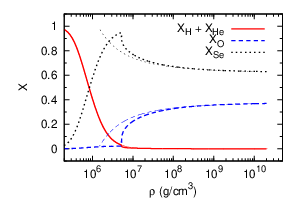
In Fig. 4 we present our results for the ⁵⁶Fe-⁷⁹Se and ¹⁶O-⁷⁹Se systems discussed in §II; again we choose $\dot{m}_{4}=3$, $\xi=1$, and an ocean temperature $T=3\times 10^{8}~{\rm K}$. For comparison we also present the $X_{\rm Fe}$, $X_{\rm O}$, and $X_{\rm Se}$ profiles when the hydrogen/helium burning layer is neglected (§III.1). These profiles are nearly the same as the profiles when the burning layer is included, except at the top of the convection zone where the latter profiles are very steep. The change in the slope of the profiles from §III.1 to §III.2 can be understood from Eq. (22): This equation states that within the convection zone $\sum_{i=1}^{n-1}\chi_{X_{i}}\nabla_{X_{i}}$ follow the adiabatic gradient, but places no such restriction on the individual $X$ profiles. Therefore, at the top of the convection zone, the Fe, O, and Se composition profiles rise sharply with increasing density because of the correspondingly large drop in the H-He profile. The burning layer acts as a barrier to convection, such that the convection zone ends abruptly at the base of this layer.

Finally, in Fig. 4 we present $X_{\rm H}+X_{\rm He}$ profiles when convection is ignored [such that Eqs. (29) and (31) apply across the entire ocean]. The shape of these profiles results from the balance between accretion driving the H-He mixture deeper and nuclear reactions converting H-He into heavier elements as it travels inward; the profiles can be estimated using Eqs. (2) and (24): $1-t_{\rm accr}R_{3\alpha}\simeq X_{1}\Rightarrow X_{1}\propto\rho^{5/3}$ for $X_{1}\lesssim 0.1$. In addition to the sharp drop at the top of the convection zone, the profiles when convection is included differ in that they fall more slowly with increasing density, due to their larger inward velocity; since $v_{\rm conv}\propto\rho^{-2/3}$ in the deep ocean, $X_{1}\propto\rho^{3/2}$ for $X_{1}\lesssim 10^{-3}$. The $X_{\rm H}+X_{\rm He}$ profiles therefore cross at some depth in the ocean; i.e., convection causes some hydrogen-helium to mix into deeper layers. While this mixing will change the amount of burning at each depth in the convection zone, we do not expect the thermal profile in this region to change, because the amount of helium in the convection region is very small (less than 10% by mass of the total helium in the star, and less than 1% of the total mass at any depth in the convection zone; see Fig. 4).