Euler-Bessel and Euler-Fourier Transforms
Abstract
We consider a topological integral transform of Bessel (concentric isospectral sets) type and Fourier (hyperplane isospectral sets) type, using the Euler characteristic as a measure. These transforms convert constructible -valued functions to continuous -valued functions over a vector space. Core contributions include: the definition of the topological Bessel transform; a relationship in terms of the logarithmic blowup of the topological Fourier transform; and a novel Morse index formula for the transforms. We then apply the theory to problems of target reconstruction from enumerative sensor data, including localization and shape discrimination. This last application utilizes an extension of spatially variant apodization (SVA) to mitigate sidelobe phenomena.
ams
65R10,58C351 Introduction
Integral transforms are inherently geometric and, as such, are invaluable to applications in reconstruction. The vast literature on integral geometry possesses hints that many such integral transforms are at heart topological: note the constant refrain of Euler characteristic throughout integral-geometric results such as Crofton’s Theorem or Hadwiger’s Theorems (see, e.g., [9]). The parallel appearance of integral transforms in microlocal analysis — especially from the sheaf-theoretic literature [8] — confirms the role of topology in integral transforms.
This paper considers particular integral transforms designed to extract geometric features from topological data. The key technical tool involved is Euler calculus — a simple integration theory using the (geometric or o-minimal) Euler characteristic as a measure (or valuation, to be precise). We define two types of Euler characteristic integral transforms: one, a generalization of the Fourier transform; the other, a generalization of the Hankel or Bessel transform. These generalizations are denoted Euler-Fourier and Euler-Bessel transforms, respectively. These transforms are novel, apart from the foreshadowing in the recent work on Euler integration [2].
The contributions of this paper are as follow:
- 1.
Definitions of the Euler-Bessel and Euler-Fourier transforms on a normed (resp. inner-product) vector space;
- 2.
Index theorems for both transforms which concentrate the transforms onto sets of critical points, and thereby reveal Morse-theoretic connections;
- 3.
Applications of the Euler-Bessel transform to target localization and shape-discrimination problems; and
- 4.
An extension of spatially variant apodization (SVA) to Euler-Bessel transforms, with applications to sidelobe mitigation and to shape discrimination.
2 Background: Euler calculus
The Euler calculus is an integral calculus based on the topological Euler characteristic. The reader may find a simple explanation of Euler calculus in [1] and more detailed treatments in [10, 14]. For simplicity, we work in a fixed class of suitably “tame” or definable sets and mappings. In brief, an o-minimal structure is a collection of so-called definable subsets of Euclidean space satisfying certain axioms; a definable mapping between definable sets is a map whose graph is also a definable subset of the product: see [13]. For concreteness, the reader may substitute “semialgebraic” or “piecewise-linear” or “globally subanalytic” for definable. All definable sets are finitely decomposable into open simplices in a manner that makes the Euler characteristic invariant. Given a finite partition of a definable set into definable sets definably homeomorphic to open simplices,
| (1) |
This Euler characteristic also possesses a description in terms of alternating sums of (local) homology groups, yielding a topological invariance (up to homeomorphism for general definable spaces; up to homotopy for compact definable spaces).
The Euler characteristic is additive: . Thus, one defines a scale-invariant “measure” and an integral via characteristic functions: for definable. The collection of functions from a definable space to generated by finite (!) linear combinations of characteristic functions over compact definable sets is the group of constructible functions, . The Euler integral is the linear operator taking the characteristic function of an open -simplex to . By additivity of , the integral is well-defined [10, 14]. There are several formulae for the computation (and numerical approximation) of integrals with respect to [1].
The integral with respect to is well-defined for more general constructible functions taking values in a discrete subset of ; however, continuously-varying integrands are problematic. A recent extension of the Euler integral to -valued definable functions uses a limiting process [2]. Let denote the definable functions from to (those whose graphs in are definable sets). There is a pair of dual extensions of the Euler integral, and , defined as follows:
| (2) |
These limits exist and are well-defined, though not equal in general. The triangulation theorem for [13] states that to any , there is a definable triangulation (a definable bijection to a disjoint union of open affine simplices in some Euclidean space) on which is affine on each open simplex. From this, one may reduce all questions about the integrals over to questions of affine integrands over simplices, using the additivity of the integral. Using this reduction technique, one proves the following computational formulae [2]:
Theorem 2.1.
For ,
| (3) | |||||
| (4) |
This integral is coordinate-free, in the sense of being invariant under right-actions of homeomorphisms of ; however, the integral operators are not linear, nor, since , are they even homogeneous with respect to negative coefficients. The compelling feature of the measures and is their relation to stratified Morse theory [7].
Let denote the set of critical points of . For arbitrary , the co-index of , , is defined as
| (5) |
where denotes the closed ball in of radius about . The dual index at is given by
| (6) |
Theorem 2.2 (Theorem 4 of [2]).
If is continuous and definable on , then:
| (7) |
This has the effect of concentrating the measure on the critical points of the distribution. In the case of a Morse function on an -manifold , for each critical point , and , where is the Morse index of . Thus, if is a Morse function, then:
| (8) |
3 Definition: Euler-Bessel and Euler-Fourier transforms
There are a number of interesting integral transforms based on , including convolution and Radon-type transforms [4, 11]. We introduce two Euler integral transforms on vector spaces for use in signal processing problems.
3.1 Bessel
For the Eulerian generalization of a Bessel transform, let denote a finite-dimensional vector space with (definable, continuous) norm , and let denote the compact ball of points . Recall that denotes compactly-supported definable integer-valued functions.
Definition 3.1.
For define the Bessel transform of via
| (9) |
This transform Euler-integrates over the concentric spheres at of radius , and Lebesgue-integrates these spherical Euler integrals with respect to . For the Euclidean norm, these isospectral sets are round spheres. Given our convention that consists of compactly supported functions, is well-defined using standard o-minimal techniques (the Conic Theorem [13]).
3.2 Fourier
There is a similar integral transform that is best thought of as a topological version of the Fourier transform. This is a global version of the microlocal Fourier-Sato transform on the sheaf [8]. For this transform, an inner product on must be specified. The Fourier transform takes as its argument a covector .
Definition 3.2.
For define the Fourier transform of in the direction via
| (10) |
Example 3.3.
For a compact convex subset of and , equals the projected length of along the -axis.
The Bessel transform can be seen as a Fourier transform of the log-blowup. This perspective leads to results like the following.
Proposition 3.4.
The Bessel transform along an asymptotic ray is the Fourier transform along the ray’s direction: for and ,
| (11) |
where is the dual covector.
Proof.
The isospectral sets restricted to the (compact) support of converge in the limit and the scalings are identical. ∎
While the Fourier transform obviously measures a “width” associated to a constructible function, the geometric interpretation of the Bessel transform is more involved. The next section explores this geometric content via index theory.
4 Computation: Index-theoretic formulae
The principal results of this paper is are index formulae for the Euler-Bessel and Euler-Fourier transforms that reduce the integrals to critical values.
Lemma 4.1.
For the closure of a open subset of , star-convex with respect to ,
| (12) |
where is the distance-to- function .
Proof.
Consider the logarithmic blowup taking , with the second coordinate being . The level sets of the coordinate of the blowup are precisely the isospectral sets of . The induced height function is well-defined on the unit tangent sphere of , , since is star-convex with respect to . By definition,
For star-convex and top-dimensional, is homeomorphic to . By Equation (3),
∎
This theorem is a manifestation of Stokes’ Theorem: the integral of the distance over equals the integral of the ‘derivative’ of distance over . For non-star-convex domains, it is necessary to break up the boundary into positively and negatively oriented pieces. These orientations implicate and respectively.
Theorem 4.2.
For the closure of a definable bounded open subset of and , decompose into , where are the (closure of) subsets of on which the outward-pointing halfspaces contain (for ) or, respectively, do not contain (for ) . Then,
| (13) | |||||
| (14) |
where denotes the critical points of .
Proof.
Assume, for simplicity, that is the closure of the difference of , the cone at over , and , the cone over . (The case of multiple cones follow by induction.) These cones, being star-convex with respect to , admit analysis as per Lemma 4.1. The crucial observation is that, by additivity of ,
Integrating both sides with respect to and invoking Theorem 2.1 gives
By Theorem 2.2, this reduces to an integral over the critical sets of . The only critical point of on or is itself, on which the integrand takes the value and does not contribute to the integral. Therefore the integrals over the cone boundaries may be restricted to and respectively. The index-theoretic result follows from Theorem 2.2. ∎
In even dimensions, the -vs- dichotomy dissolves:
Corollary 4.3.
For even and the closure of a bounded definable open set,
| (15) |
Proof.
Given the index theorem for the Euler-Bessel transform, that for the Euler-Fourier is a trivial modification that generalizes Example 3.3.
Theorem 4.4.
For the closure of a definable bounded open subset of and , decompose into , where are the (closure of) subsets of on which points out of () or into () . Then,
| (16) | |||||
| (17) |
where denotes the critical points of . For even, this becomes:
| (18) |
The proof follows that of Theorem 4.2 and is an exercise. Figure 1 gives a simple example of the Bessel and Fourier index theorems in .

By linearity of and over , one derives index formulae for integrands in expressible as a linear combination of for the closure of definable bounded open sets. For a set which is not of dimension , it is still possible to apply the index formula by means of a limiting process on compact tubular neighborhoods of .
The remainder of this paper explores applications of the Euler-Bessel transform to signal processing problems involving target detection, localization, and discrimination.
5 Application: Target localization
Applications of Euler-type integral transforms are naturally made in the context of (reasonably dense) sensor networks. As in [1], we consider the setting in which a finite number of targets reside in a field of sensors whose locations are parameterized by a vector space . Each target has a corresponding support — the subset of on which a sensor senses the target, albeit without information of the target’s range, bearing, or identity. The resulting sensor counting function contains highly redundant but informative structure. The Euler integral can be used to extract from the number of targets [1]; the Euler-Bessel transform can be used to localize the targets in the case of convex target supports. Assume for example that all target supports are equal to a round ball: all sensors within some fixed distance of the target detect it. The Bessel transform of the sensor field reveals the exact location of the target.
Proposition 5.1.
For a compact ball about , the Bessel transform is a nondecreasing function of the distance to , having unique zero at .
Proof.
Convexity of balls and Corollary 4.3 implies that
which equals for and is monotone in distance-to- within . ∎
Note that Proposition 5.1 fails in odd dimensions; the Bessel transform of a ball in is constant, and obscures all information. However, for even dimensions, Proposition 5.1 provides a basis for target localization. For targets with convex supports (regions detected by counting sensors), the local minima of the Euler-Bessel transform can reveal target locations: see Fig. 2[left] for an example. Note that in this example, not all local minima are target centers: interference creates ghost minima. However, given , the integral determines the number of targets. This provides a guide as to how many of the deepest local minima to interrogate.


There are significant limitations to superposition by linearity for this application. When targets are nearby or overlapping, their individual transforms will have overlapping sidelobes, which results in uncertainty when the transform is being used for localization. A typical example of this difficulty (present even in the setting of round targets) is shown in Figure 2[right].
6 Spatially variant apodization and sidelobes
Figure 2 reveals the prevalence of sidelobes in the application of the Euler-Bessel transform — regions of “energy leakage” in the transform — much the same as occurs in Lebesgue-theoretic integral transforms. These are, in general, disruptive, especially in the context of several targets, where multiple side lobe interferences can create “ghost” images. Such problems are prevalent in traditional radar image processing, and their wealth of available perspectives in mitigating unwanted sidelobes provides a base of intuition for dealing with the present context.
One obvious method for modifying the output of Euler-Bessel transform is to change the isospectral contours of integration , as regulated by the norm . For example, one can contrast the circular (or ) Euler-Bessel transform with its square (or ) variant. The resulting outputs of norm-varied transforms can have incisive characteristics in some circumstances: see §7. However, it may the case that no single norm is optimal for a given input, especially if it consists of multiple targets with different characteristics.
We propose the adaptation and refinement of one tool of widespread use in traditional radar processing. This usually goes under the name of SVA: spatially variant apodization (see [12] for the original implementation; an updated discussion is in [5]). Though there are many heuristic implementations of SVA, the core concept behind the method involves using a parameterized family of kernels and optimizing the transform pointwise with respect to this family. The family of kernels is designed so as to reduce as much as possible the magnitude of the sidelobe phenomena, while preserving as much as possible the primary lobe.
For the setting of the Euler-Bessel transform, we propose the following. Consider a parameterized family of norms , . The SVA Euler-Bessel transform is the pointwise infimum of transforms over .
| (19) |
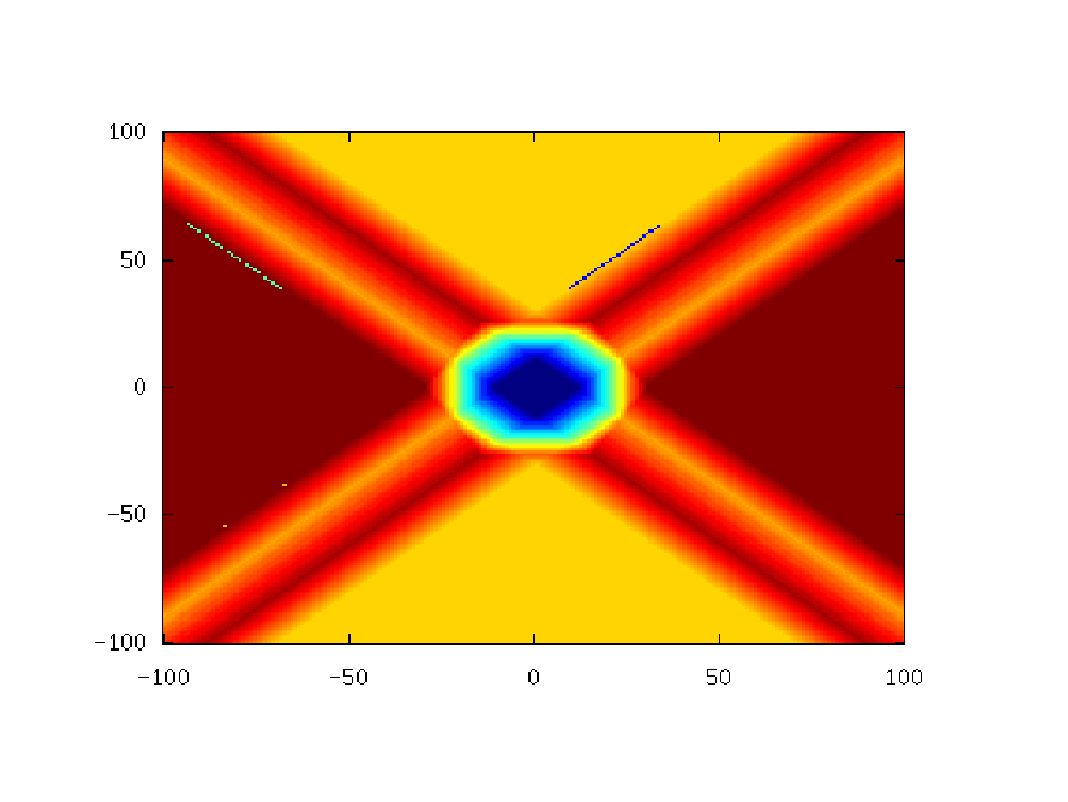
where is the radius ball about in the -norm. For example, could describe a cyclic family of rotated norms. As shown in Figure 3, SVA with this rotated family eliminates the sidelobes from the transform of a square rotated by an unknown amount, while preserving the response of another nearby target.


As in the case of traditional radar processing, there is benefit to SVA implementation even when the transform contour is not similar to the expected target shape. For instance, contours result in strong sidelobes in the transform of a hexagon (Figure 4[left]). Application of rotated SVA (Figure 4[right]) does not eliminate the sidelobes, but does dramatically reduce their magnitude.

7 Application: Waveforms and shape discrimination
Motivated by matched-filter processing, we apply Euler-Bessel transforms to perform geometric discrimination from enumerative data. Since the Euler-Bessel transform of a target has minimal sidelobes when the isospectral contours agree with the target shape, it can be used to construct a shape filter. To test this, a simulation was run on a function for a collection of polygonal domains in . The results are shown in Figures 5 through 8. In these, (upper left) is a hexagon; (upper right) is a rotated square; (lower left) is a round disk; and (lower right) is an axis-aligned square. The sizes of these support regions were varied, to the point of significant overlap and interference.


Three variants of the Euler-Bessel transform were applied to the functions: an transform, an transform , and an SVA (rotated ) transform. The deep local minima of each transform correspond to the likely centers for the selected target shapes, in accordance with Proposition 5.1. For instance, with the transform, although there are minima at the center of the two squares, they are not as deep as the minimum at the center of the disk. Similarly, the square transform has its deepest minimum at the center of the axis-aligned square, and the SVA transform detects both squares. Even when the support regions overlap, the Euler-Bessel transforms still successfully discriminate target geometries, though too much overlap generates interference and obscures the target geometries (Figure 8).


Future work will explore the use of SVA in the context of Euler integral transforms.
8 Concluding remarks
- 1.
- 2.
We have left unaddressed several important issues, such as the existence and nature of inverse and discrete transforms. For inverses to a broad but distinct class of Euler integral transforms, see [11, BGL:radon].
- 3.
Computational issues for discrete Euler-Bessel and Euler-Fourier transforms remain a significant challenge. Though individual Euler integrals can be efficiently approximated on planar networks [1], the integral transforms of this paper are, at present, computation-intensive.
- 4.
There is no fundamental obstruction to defining and over , so that the transforms act on real-valued (definable) functions. In this case, one would have to distinguish between and versions of the transforms. It is not clear what such transforms measure – geometrically or topologically – or which index formulae might persist. The passage to definable inputs means that these transforms will no longer be linear (as neither nor is).
- 5.
The use of SVA methods is one of many possible points of contact between the radar signal processing community and Euler integration.
Bibliography
References
- [1] Y. Baryshnikov and R. Ghrist, “Target enumeration via Euler characteristic integrals,” SIAM J. Appl. Math., 70(3), 825-844, 2009.
- [2] Y. Baryshnikov and R. Ghrist, “Euler integration for definable functions,” Proc. National Acad. Sci ., 107(21), May 25, 9525-9530, 2010.
- [3] Y. Baryshnikov, R. Ghrist, and D. Lipsky “Inversion of Euler integral transforms with applications to sensor data,” preprint.
- [4] L. Bröcker, “Euler integration and Euler multiplication,” Adv. Geom. 5, 2005, 145–169.
- [5] W. Carrara, R. Goodman, and R. Majewski, “Spotlight Synthetic Aperture Radar,” Signal Processing Algorithms, Artech House, 1995, 264–278.
- [6] R. Cluckers and M. Edmundo, “Integration of positive constructible functions against Euler characteristic and dimension,” J. Pure Appl. Algebra, 208, no. 2, 2006, 691–698.
- [7] M. Goresky and R. MacPherson, Stratified Morse Theory, Springer-Verlag, 1988.
- [8] M. Kashiwara and P. Schapira, Sheaves on Manifolds, Springer-Verlag, 1994.
- [9] D. Klain and G.-C. Rota, Introduction to Geometric Probability, Cambridge University Press, 1997.
- [10] P. Schapira, “Operations on constructible functions,” J. Pure Appl. Algebra 72, 1991, 83–93.
- [11] P. Schapira, “Tomography of constructible functions,” in proceedings of 11th Intl. Symp. on Applied Algebra, Algebraic Algorithms and Error-Correcting Codes, 1995, 427–435.
- [12] H. Stankwitz, R. Dallaire, and J. Fienup, “Spatially variant apodization for sidelobe control in SAR imagery.” In IEEE National Radar Conference, 1994, 132–137.
- [13] L. Van den Dries, Tame Topology and O-Minimal Structures, Cambridge University Press, 1998.
- [14] O. Viro, “Some integral calculus based on Euler characteristic,” Lecture Notes in Math., vol. 1346, Springer-Verlag, 1988, 127–138.