Graphical Models Concepts in Compressed Sensing

Andrea Montanari ^†^†thanks: Department of Electrical Engineering and Department of Statistics, Stanford University

Abstract

This paper surveys recent work in applying ideas from graphical models and message passing algorithms to solve large scale regularized regression problems. In particular, the focus is on compressed sensing reconstruction via $\ell_{1}$ penalized least-squares (known as LASSO or BPDN). We discuss how to derive fast approximate message passing algorithms to solve this problem. Surprisingly, the analysis of such algorithms allows to prove exact high-dimensional limit results for the LASSO risk.

This paper will appear as a chapter in a book on ‘Compressed Sensing’ edited by Yonina Eldar and Gitta Kutyniok.

1 Introduction

The problem of reconstructing a high-dimensional vector $x\in{\mathbb{R}}^{n}$ from a collection of observations $y\in{\mathbb{R}}^{m}$ arises in a number of contexts, ranging from statistical learning to signal processing. It is often assumed that the measurement process is approximately linear, i.e. that

\displaystyle y=Ax+w\,,

(1.1)

where $A\in{\mathbb{R}}^{m\times n}$ is a known measurement matrix, and $w$ is a noise vector.

The graphical models approach to such reconstruction problem postulates a joint probability distribution on $(x,y)$ which takes, without loss of generality, the form

\displaystyle p({\rm d}x,\,{\rm d}y)=p({\rm d}y|x)\,p({\rm d}x)\,.

(1.2)

The conditional distribution $p({\rm d}y|x)$ models the noise process, while the prior $p({\rm d}x)$ encodes information on the vector $x$ . In particular, within compressed sensing, it can describe its sparsity properties. Within a graphical models approach, either of these distributions (or both) factorizes according to a specific graph structure. The resulting posterior distribution $p({\rm d}x|y)$ is used for inferring $x$ given $y$ .

There are many reasons to be skeptical about the idea that the joint probability distribution $p({\rm d}x,\,{\rm d}y)$ can be determined, and used for reconstructing $x$ . To name one such reason for skepticism, any finite sample will allow to determine the prior distribution of $x$ , $p({\rm d}x)$ only within limited accuracy. A reconstruction algorithm based on the posterior distribution $p({\rm d}x|y)$ might be sensitive with respect to changes in the prior thus leading to systematic errors.

One might be tempted to drop the whole approach as a consequence. We argue that sticking to this point of view is instead fruitful for several reasons:

1.

Algorithmic. Several existing reconstruction methods are in fact M-estimators, i.e. they are defined by minimizing an appropriate cost function ${\cal C}_{A,y}(x)$ over $x\in{\mathbb{R}}^{n}$ [vdV00]. Such estimators can be derived as Bayesian estimators (e.g. maximum a posteriori probability) for specific forms of $p({\rm d}x)$ and $p({\rm d}y|x)$ (for instance by letting $p({\rm d}x|y)\propto\exp\{-{\cal C}_{A,y}(x))\,{\rm d}x\,$ ). The connection is useful both in interpreting/comparing different methods, and in adapting known algorithms for Bayes estimation. A classical example of this cross-fertilization is the paper [FN03]. This review discusses several other examples in that build on graphical models inference algorithms.
2.

Minimax. When the prior $p({\rm d}x)$ or the noise distributions, and therefore the conditional distribution $p({\rm d}y|x)$ , ‘exist’ but are unknown, it is reasonable to assume that they belong to specific structure classes. By this term we refer generically to a class of probability distributions characterized by a specific property. For instance, within compressed sensing one often assumes that $x$ has at most $k$ non-zero entries. One can then take $p({\rm d}x)$ to be a distribution supported on $k$ -sparse vectors $x\in{\mathbb{R}}^{n}$ . If ${\cal F}_{n,k}$ denotes the class of such distributions, the minimax approach strives to achieve the best uniform guarantee over ${\cal F}_{n,k}$ . In other words, the minimax estimator achieves the smallest expected error (e.g. mean square error) for the ‘worst’ distribution in ${\cal F}_{n,k}$ .

It is a remarkable fact in statistical decision theory [LC98] (which follows from a generalization of Von Neumann minimax theorem) that the minimax estimator coincides with the Bayes estimator for a specific (worst case) prior $p\in{\cal F}_{n,k}$ . In one dimension considerable information is available about the worst case distribution and asymptotically optimal estimators (see Section 3). The methods developed here allow to develop similar insights in high-dimension.
3.

Modeling. In some applications it is possible to construct fairly accurate models both of the prior distribution $p({\rm d}x)$ and of the measurement process $p({\rm d}y|x)$ . This is the case for instance in some communications problems, whereby $x$ is the signal produced by a transmitter (and generated uniformly at random according to a known codebook), and $w$ is the noise produced by a well-defined physical process (e.g. thermal noise in the receiver circuitry). A discussion of some families of practically interesting priors $p({\rm d}x)$ can be found in [Cev08].

Further, the question of modeling the prior in compressed sensing is discussed from the point of view of Bayesian theory in [JXC08].

The rest of this chapter is organized as follows. Section 2 describes a graphical model naturally associated to the compressed sensing reconstruction problem. Section 3 provides important background on the one-dimensional case. Section 4 describes a standard message passing algorithm –the min-sum algorithm– and how it can be simplified to solve the LASSO optimization problem. The algorithm is further simplified in Section 5 yielding the AMP algoritm. The analysis of this algorithm is outlined in Section 6. As a consequence of this analysis, it is possible to compute exact high-dimensional limits for the behavior of the LASSO estimator. Finally in Section 7 we discuss a few examples of how the approach developed here can be used to address reconstruction problems in which a richer structural information is available.

1.1 Some useful notation

Throughout this review, probability measures over the real line ${\mathbb{R}}$ or the euclidean space ${\mathbb{R}}^{K}$ play a special role. It is therefore useful to be careful about the probability-theory notation. The less careful reader who prefers to pass directly to the ‘action’ is invited to skip these remarks at a first reading.

We will use the notation $p$ or $p({\rm d}x)$ to indicate probability measures (eventually with subscripts). Notice that, in the last form, the ${\rm d}x$ is only a reminder of which variable is distributed with measure $p$ . (Of course one is tempted to think of ${\rm d}x$ as an infinitesimal interval but this intuition is accurate only if $p$ admits a density.)

A special measure (positive, but not normalized and hence not a probability measure) is the Lebesgue measure for which we reserve the special notation ${\rm d}x$ (something like $\mu({\rm d}x)$ would be more consistent but, in our opinion, less readable). This convention is particularly convenient for expressing in formulae statements of the form ‘ $p$ admits a density $f$ with respect to Lebesgue measure ${\rm d}x$ , with $f:x\mapsto f(x)\equiv\exp(-x^{2}/(2a))/\sqrt{2\pi a}$ a Borel function’, which we write simply

\displaystyle p({\rm d}x)=\frac{1}{\sqrt{2\pi a}}\,e^{-x^{2}/2a}\,{\rm d}x\,.

(1.3)

It is well known that expectations are defined as integrals with respect to the probability measure which we denote as

\displaystyle{\mathbb{E}}_{p}\{f\}=\int_{{\mathbb{R}}}\!f(x)\,p({\rm d}x)\,,

(1.4)

sometimes omitting the subscript $p$ in ${\mathbb{E}}_{p}$ and ${\mathbb{R}}$ in $\int_{{\mathbb{R}}}$ . Unless specified otherwise, we do not assume such probability measures to have a density with respect to Lebesgue measure. The probability measure $p$ is a set function defined on the Borel $\sigma$ -algebra, see e.g. [Bil95, Wil91]. Hence it makes sense to write $p((-1,3])$ (the probability of the interval $(-1,3]$ under measure $p$ ) or $p(\{0\})$ (the probability of the point $0$ ). Equally valid would be expressions such as ${\rm d}x((-1,3])$ (the Lebesgue measure of $(-1,3]$ ) or $p({\rm d}x)((-1,3])$ (the probability of the interval $(-1,3]$ under measure $p$ ) but we avoid them as somewhat clumsy.

A (joint) probability measure over $x\in{\mathbb{R}}^{K}$ and $y\in{\mathbb{R}}^{L}$ will be denoted by $p({\rm d}x,{\rm d}y)$ (this is just a probability measure over ${\mathbb{R}}^{K}\times{\mathbb{R}}^{L}={\mathbb{R}}^{K+L}$ ). The corresponding conditional probability measure of $y$ given $x$ is denoted by $p({\rm d}x|y)$ (for a rigorous definition we refer to [Bil95, Wil91]).

Finally, we will not make use of cumulative distribution functions –commonly called distribution functions in probability theory– and instead use ‘probability distribution’ interchangeably with ‘probability measure’.

Some fairly standard discrete mathematics notation will also be useful. The set of first $K$ integers is to be denoted by $[K]=\{1,\dots,K\}$ . Order of growth of various functions will be characterized by the standard ‘big- $O$ ’ notation. Recall in particular that, for $M\to\infty$ , one writes $f(M)=O(g(M))$ if $f(M)\leq C\,g(M)$ for some finite constant $C$ , $f(M)=\Omega(g(M))$ if $f(M)\geq g(M)/C$ and $f(M)=\Theta(g(M))$ if $g(M)/C\leq f(M)\leq Cg(M)$ . Further $f(M)=o(g(M))$ if $f(M)/g(M)\to 0$ . Analogous notations are used when the argument of $f$ and $g$ go to $0$ .

2 The basic model and its graph structure

Specifying the conditional distribution of $y$ given $x$ is equivalent to specifying the distribution of the noise vector $w$ . In most of this chapter we shall take $p(w)$ to be a Gaussian distribution of mean $0$ and variance $\beta^{-1}{\rm\bf I}$ , whence

\displaystyle p_{\beta}({\rm d}y|x)=\Big(\frac{\beta}{2\pi}\Big)^{n/2}\,\exp\Big\{-\frac{\beta}{2}\|y-Ax\|_{2}^{2}\Big\}\,{\rm d}y\,.

(2.1)

The simplest choice for the prior consists in taking $p({\rm d}x)$ to be a product distribution with identical factors $p({\rm d}x)=p({\rm d}x_{1})\times\dots\times p({\rm d}x_{n})$ . We thus obtain the joint distribution

\displaystyle p_{\beta}({\rm d}x,\,{\rm d}y)=\Big(\frac{\beta}{2\pi}\Big)^{n/2}\,\exp\Big\{-\frac{\beta}{2}\|y-Ax\|_{2}^{2}\Big\}\,{\rm d}y\,\prod_{i=1}^{n}p({\rm d}x_{i})\,.

(2.2)

It is clear at the outset that generalizations of this basic model can be easily defined, in such a way to incorporate further information on the vector $x$ or on the measurement process. As an example, consider the case of block-sparse signals: The index set $[n]$ is partitioned into blocks $B(1)$ , $B(2)$ , … $B(\ell)$ of equal length $n/\ell$ , and only a small fraction of the blocks is non-vanishing. This situation can be captured by assuming that the prior $p({\rm d}x)$ factors over blocks. One thus obtains the joint distribution

\displaystyle p_{\beta}({\rm d}x,\,{\rm d}y)=\Big(\frac{\beta}{2\pi}\Big)^{n/2}\,\exp\Big\{-\frac{\beta}{2}\|y-Ax\|_{2}^{2}\Big\}\,{\rm d}y\,\prod_{j=1}^{\ell}p({\rm d}x_{B(j)})\,,

(2.3)

where $x_{B(j)}\equiv(x_{i}:\,i\in B(j))\in{\mathbb{R}}^{n/\ell}$ . Other examples of structured priors will be discussed in Section 7.

The posterior distribution of $x$ given observations $y$ admits an explicit expression, that can be derived from Eq. (2.2):

\displaystyle p_{\beta}({\rm d}x|\,y)=\frac{1}{Z(y)}\,\exp\Big\{-\frac{\beta}{2}\|y-Ax\|_{2}^{2}\Big\}\,\,\prod_{i=1}^{n}p({\rm d}x_{i})\,,

(2.4)

where $Z(y)=(2\pi/\beta)^{n/2}p(y)$ ensures the normalization $\int p({\rm d}x|y)=1$ . Let us stress that while this expression is explicit, computing expectations or marginals of this distribution is a hard computational task.

Finally, the square residuals $\|y-Ax\|_{2}^{2}$ decompose in a sum of $m$ terms yielding

\displaystyle p_{\beta}({\rm d}x|\,y)=\frac{1}{Z(y)}\,\prod_{a=1}^{m}\exp\Big\{-\frac{\beta}{2}\big(y_{a}-A_{a}^{T}x\big)^{2}\Big\}\,\,\prod_{i=1}^{n}p({\rm d}x_{i})\,,

(2.5)

where $A_{a}$ is the $a$ -th row of the matrix $a$ . This factorized structure is conveniently described by a factor graph, i.e. a bipartite graph including a ‘variable node’ $i\in[n]$ for each variable $x_{i}$ , and a ‘factor node’ $a\in[m]$ for each term $\psi_{a}(x)=\exp\{-\beta(y_{a}-A_{a}^{T}x)^{2}/2\}$ . Variable $i$ and factor $a$ are connected by an edge if and only if $\psi_{a}(x)$ depends non-trivially on $x_{i}$ , i.e. if $A_{ai}\neq 0$ . One such factor graph is reproduced in Fig. 1.

Refer to caption — Figure 1: Factor graph associated to the probability distribution (2.5). Empty circles correspond to variables $x_{i}$ , $i\in[n]$ and squares correspond to measurements $y_{a}$ , $a\in[m]$ .

An estimate of the signal can be extracted from the posterior distribution (2.5) in various ways. One possibility is to use conditional expectation

\displaystyle\widehat{x}_{\beta}(y;p)\equiv\int_{{\mathbb{R}}^{n}}x\;p_{\beta}({\rm d}x|y)\,.

(2.6)

Classically, this estimator is justified by the fact that it achieves the minimal mean square provided the $p_{\beta}({\rm d}x,{\rm d}y)$ is the actual joint distribution of $(x,y)$ . In the present context we will not assume that ‘postulated’ prior $p_{\beta}({\rm d}x)$ coincides with the actual distribution f $x$ , and hence $\widehat{x}_{\beta}(y;p)$ is not necessarily optimal (with respect to mean square error). The best justification for $\widehat{x}_{\beta}(y;p)$ is that a broad class of estimators can be written in the form (2.6).

An important problem with the estimator (2.6) is that it is in general hard to compute. In order to obtain a tractable proxy, we assume that $p({\rm d}x_{i})=p_{\beta,h}({\rm d}x_{i})=c\,f_{\beta,h}(x_{i})\,{\rm d}x_{i}$ for $f_{\beta,h}(x_{i})=e^{-\beta h(x_{i})}$ an un-normalized probability density function. As $\beta$ get large, the integral in Eq. (2.6) becomes dominated by the vector $x$ with the highest posterior probability $p_{\beta}$ . One can then replace the integral in ${\rm d}x$ with a maximization over $x$ and define

	$\displaystyle\widehat{x}(y;h)$	$\displaystyle\equiv{\rm argmin}_{z\in{\mathbb{R}}^{n}}{\cal C}_{A,y}(z;h)\,,$		(2.7)
	$\displaystyle{\cal C}_{A,y}(z;h)$	$\displaystyle\equiv\frac{1}{2}\\|y-Az\\|_{2}^{2}+\sum_{i=1}^{n}h(z_{i})\,,$

where we assumed for simplicity that ${\cal C}_{A,y}(z;h)$ has a unique minimum.

According to the above discussion, the estimator $\widehat{x}(y;h)$ can be thought of as the $\beta\to\infty$ limit of the general estimator (2.6). Indeed, it is easy to check that, provided $x_{i}\mapsto h(x_{i})$ is upper semicontinuous, we have

\displaystyle\lim_{\beta\to\infty}\widehat{x}_{\beta}(y;p_{\beta,h})=\widehat{x}(y;h)\,.

In other words, the posterior mean converges to the mode of the posterior in this limit. Further, $\widehat{x}(y;h)$ takes the familiar form of a regression estimator with separable regularization. If $h(\,\cdot\,)$ is convex, the computation of $\widehat{x}$ is tractable. Important special cases include $h(x_{i})=\lambda x_{i}^{2}$ , which corresponds to ridge regression [HTF03], and $h(x_{i})=\lambda|x_{i}|$ which corresponds to the LASSO [Tib96] or basis pursuit denoising (BPDN) [CD95]. Due to the special role it plays in compressed sensing, we will devote special attention to the latter case, that we rewrite explicitly below with a slight abuse of notation

	$\displaystyle\widehat{x}(y)$	$\displaystyle\equiv{\rm argmin}_{z\in{\mathbb{R}}^{n}}{\cal C}_{A,y}(z)\,,$		(2.8)
	$\displaystyle{\cal C}_{A,y}(z)$	$\displaystyle\equiv\frac{1}{2}\\|y-Az\\|_{2}^{2}+\lambda\\|z\\|_{1}\,.$

3 Revisiting the scalar case

Before proceeding further, it is convenient to pause for a moment and consider the special case of a single measurement of a scalar quantity, i.e. the case $m=n=1$ . We therefore have

\displaystyle y=x+w\,,

(3.1)

and want to estimate $x$ from $y$ . Despite the apparent simplicity, there exists a copious literature on this problem with many open problems [DJHS92, DJ94b, DJ94a, Joh02]. Here we only want to clarify a few points that will come up again in what follows.

In order to compare various estimators we will assume that $(x,y)$ are indeed random variables with some underlying probability distribution $p_{0}({\rm d}x,{\rm d}y)=p_{0}({\rm d}x)p_{0}({\rm d}y|x)$ . It is important to stress that this distribution is conceptually distinct from the one used in inference, cf. Eq. (2.6). In particular we cannot assume to know the actual prior distribution of $x$ , at least not exactly, and hence $p({\rm d}x)$ and $p_{0}({\rm d}x)$ do not coincide. The ‘actual’ prior $p_{0}$ is the distribution of the vector to be inferred, while the ‘postulated’ prior $p$ is a device used for designing inference algorithms.

For the sake of simplicity we also consider Gaussian noise $w\sim{\sf N}(0,\sigma^{2})$ with known noise level $\sigma^{2}$ . Various estimators will be compared with respect to the resulting mean square error

\displaystyle{\rm MSE}={\mathbb{E}}\{|\widehat{x}(y)-x|^{2}\}=\int_{{\mathbb{R}}\times{\mathbb{R}}}|\widehat{x}(y)-x|^{2}\,p_{0}({\rm d}x,{\rm d}y)\,.

We can distinguish two cases:

I.

The signal distribution $p_{0}(x)$ is known as well. This can be regarded as an ‘oracle’ setting. To make contact with compressed sensing, we consider distributions that generate sparse signals, i.e. that put mass at least $1-\varepsilon$ on $x=0$ . In formulae $p_{0}(\{0\})\geq 1-\varepsilon$ .
II.

The signal distribution is unknown but it is known that it is ‘sparse’, namely that it belongs to the class

$\displaystyle{\cal F}_{\varepsilon}\equiv\big\{\,p_{0}\,:\;\;p_{0}(\{0\})\geq 1-\varepsilon\,\big\}\,.$ (3.2)

The minimum mean square error, is the minimum MSE achievable by any estimator $\widehat{x}:{\mathbb{R}}\to{\mathbb{R}}$ :

\displaystyle{\rm MMSE}(\sigma^{2};p_{0})=\inf_{\widehat{x}:{\mathbb{R}}\to{\mathbb{R}}}{\mathbb{E}}\{|\widehat{x}(y)-x|^{2}\}\,.

It is well known that the infimum is achieved by the conditional expectation

\displaystyle\widehat{x}^{\mbox{\rm\footnotesize MMSE}}(y)=\int_{\mathbb{R}}x\;p_{0}({\rm d}x|y)\,.

However, this estimator assumes that we are in situation I above, i.e. that the prior $p_{0}$ is known.

In Figure 2 we plot the resulting MSE for a 3 point distribution,

\displaystyle p_{0}=\frac{\varepsilon}{2}\,\delta_{+1}+(1-\varepsilon)\,\delta_{0}+\frac{\varepsilon}{2}\,\delta_{-1}\,.

(3.3)

The MMSE is non-decreasing in $\sigma^{2}$ by construction, converges to $0$ in the noiseless limit $\sigma\to 0$ (indeed the simple rule $\widehat{x}(y)=y$ achieves MSE equal to $\sigma^{2}$ ) and to $\varepsilon$ in the large noise limit $\sigma\to\infty$ (MSE equal to $\varepsilon$ is achieved by $\widehat{x}=0$ ).

In the more realistic situation II, we do not know the prior $p_{0}$ . A principled way to deal with this ignorance would be to minimize the MSE for the worst case distribution in the class ${\cal F}_{\varepsilon}$ , i.e. to replace the minimization in Eq. (3) with the following minimax problem

\displaystyle\inf_{\widehat{x}:{\mathbb{R}}\to{\mathbb{R}}}\sup_{p_{0}\in{\cal F}_{\varepsilon}}{\mathbb{E}}\{|\widehat{x}(y)-x|^{2}\}\,.

(3.4)

A lot is known about this problem [DJHS92, DJ94b, DJ94a, Joh02]. In particular general statistical decision theory [LC98, Joh02] implies that the optimum estimator is just the posterior expectation for a specific worst case prior. Unfortunately, even a superficial discussion of this literature goes beyond the scope of the present review.

Nevertheless, an interesting exercise (indeed not a trivial one) is to consider the LASSO estimator (2.8), which in this case reduces to

\displaystyle\widehat{x}(y;\lambda)={\rm argmin}_{z\in{\mathbb{R}}}\Big\{\frac{1}{2}(y-z)^{2}+\lambda\,|z|\Big\}\,.

(3.5)

Notice that this estimator is insensitive to the details of the prior $p_{0}$ . Instead of the full minimax problem (3.4), one can then simply optimize the MSE over $\lambda$ .

The one-dimensional optimization problem (3.5) admits an explicit solution in terms of the soft thresholding function $\eta:{\mathbb{R}}\times{\mathbb{R}}_{+}\to{\mathbb{R}}$ defined as follows

\displaystyle\eta(y;\theta)=\left\{\begin{array}[]{ll}y-\theta&\mbox{ if $y>\theta$,}\\ 0&\mbox{ if $-\theta\leq y\leq\theta$,}\\ y+\theta&\mbox{ if $y<-\theta$.}\end{array}\right.

The threshold value $\theta$ has to be chosen equal to the regularization parameter $\lambda$ yielding the simple solution

\displaystyle\widehat{x}(y;\lambda)=\eta(y;\theta)\,,\;\;\;\;\mbox{for $\lambda=\theta$}\,.

(3.10)

(We emphasize the identity of $\lambda$ and $\theta$ in the scalar case, because it breaks down in the vector case.)

How should the parameter $\theta$ (or equivalently $\lambda$ ) be fixed? The rule is conceptually simple: $\theta$ should minimize the maximal mean square error for the class ${\cal F}_{\varepsilon}$ . Remarkably this complex saddle point problem can be solved rather explicitly. The key remark is that the worst case distribution over the class ${\cal F}_{\varepsilon}$ can be identified and takes the form $p^{\#}=(\varepsilon/2)\delta_{+\infty}+(1-\varepsilon)\delta_{0}+(\varepsilon/2)\delta_{-\infty}$ [DJ94b, DJ94a, Joh02].

Let us outline how the solution follows from this key fact. First of all, it makes sense to scale $\lambda$ as the noise standard deviation, because the estimator is supposed to filter out the noise. We then let $\theta=\alpha\sigma$ . In Fig. 2 we plot the resulting MSE when $\theta=\alpha\sigma$ , with $\alpha\approx 1.1402$ . We denote the LASSO/soft thresholding mean square error by ${\sf mse}(\sigma^{2};p_{0},\alpha)$ when the noise variance is $\sigma^{2}$ , $x\sim p_{0}$ , and the regularization parameter is $\lambda=\theta=\alpha\sigma$ . The worst case mean square error is given by $\sup_{p_{0}\in{\cal F}_{\varepsilon}}{\sf mse}(\sigma^{2};p_{0},\alpha)$ . Since the class ${\cal F}_{\varepsilon}$ is invariant by rescaling, this worst case MSE must be proportional to the only scale in the problem, i.e., $\sigma^{2}$ . We get

\displaystyle\sup_{p_{0}\in{\cal F}_{\varepsilon}}{\sf mse}(\sigma^{2};p_{0},\alpha)=M(\varepsilon,\alpha)\sigma^{2}\,.

(3.11)

The function $M$ can be computed explicitly by evaluating the mean square error on the worst case distribution $p^{\#}$ [DJ94b, DJ94a, Joh02]. A straightforward calculation (see also [DMM09, Supplementary Information], and [DMM10b]) yields

\displaystyle M(\varepsilon,\alpha)=\varepsilon\,(1+\alpha^{2})+(1-\varepsilon)[2(1+\alpha^{2})\,\Phi(-\alpha)-2\alpha\,\phi(\alpha)]

(3.12)

where $\phi(z)=e^{-z^{2}/2}/\sqrt{2\pi}$ is the Gaussian density and $\Phi(z)=\int_{-\infty}^{z}\phi(u)\,{\rm d}u$ is the Gaussian distribution. It is also not hard to show that that $M(\varepsilon,\alpha)$ is the slope of the soft thresholding MSE at $\sigma^{2}=0$ in a plot like the one in Fig. 2.

Minimizing the above expression over $\alpha$ , we obtain the soft thresholding minimax risk, and the corresponding optimal threshold value

\displaystyle M^{\#}(\varepsilon)\equiv\min_{\alpha\in{\mathbb{R}}_{+}}M(\varepsilon,\alpha)\,,\;\;\;\;\;\;\;\;\alpha^{\#}(\varepsilon)\equiv\arg\min_{\alpha\in{\mathbb{R}}_{+}}M(\varepsilon,\alpha)\,.

(3.13)

The functions $M^{\#}(\varepsilon)$ and $\alpha^{\#}(\varepsilon)$ are plotted in Fig. 3. For comparison we also plot the analogous functions when the class ${\cal F}_{\varepsilon}$ is replaced by ${\cal F}_{\varepsilon}(a)=\{p_{0}\in{\cal F}_{\varepsilon}:\,\int x^{2}\,p_{0}({\rm d}x)\leq a^{2}\}$ of sparse random variables with bounded second moment. Of particular interest is the behavior of these curves in the very sparse limit $\varepsilon\to 0$ ,

\displaystyle M^{\#}(\varepsilon)=2\varepsilon\log(1/\varepsilon)\,\big\{1+o(1)\big\}\,,\;\;\;\;\;\alpha^{\#}(\varepsilon)=\sqrt{2\log(1/\varepsilon)}\,\big\{1+o(1)\big\}\,.\;\;\;\;

(3.14)

Getting back to Fig. 2, the reader will notice that there is a significant gap between the minimal MSE and the MSE achieved by soft-thresholding. This is the price paid by using an estimator that is uniformly good over the class ${\cal F}_{\varepsilon}$ instead of one that is tailored for the distribution $p_{0}$ at hand. Figure 4 compares the two estimators for $\sigma=0.3$ . One might wonder whether all this price has to be paid, i.e. whether we can reduce the gap by using a more complex function instead of the soft threshold $\eta(y;\theta)$ . The answer is both yes and no. On one hand, there exist provably superior –in minimax sense– estimators over ${\cal F}_{\varepsilon}$ . Such estimators are of course more complex than simple soft thresholding. On the other hand, better estimators have the same minimax risk $M^{\#}(\varepsilon)=(2\log(1/\varepsilon))^{-1}\,\big\{1+o(1)\big\}$ in the very sparse limit, i.e. they improve only the $o(1)$ term as $\varepsilon\to 0$ [DJ94b, DJ94a, Joh02].

4 Inference via message passing

The task of extending the theory of the previous section to the vector case (1.1) might appear daunting. It turns out that such extension is instead possible in specific high-dimensional limits. The key step consists in introducing an appropriate message passing algorithm to solve the optimization problem (2.8) and then analyzing its behavior.

4.1 The min-sum algorithm

We start by considering the min-sum algorithm. Min-sum is a popular optimization algorithm for graph-structured cost functions (see for instance [Pea88, Jor98, MM09, MR07] and references therein). In order to introduce the algorithm, we consider a general cost function over $x=(x_{1},\dots,x_{n})$ , that decomposes according to a factor graph as the one shown in Fig. 1:

\displaystyle{\cal C}(x)=\sum_{a\in F}{\cal C}_{a}(x_{{\partial a}})+\sum_{i\in V}{\cal C}_{i}(x_{i})\,.

(4.1)

Here $F$ is the set of $m$ factor nodes (squares in Fig. 1) and $V$ is the set of $n$ variable nodes (circles in the same figure). Further ${\partial a}$ is the set of neighbors of node $a$ and $x_{{\partial a}}=(x_{i}\,:\,i\in{\partial a})$ . The min-sum algorithm is an iterative algorithm of the belief-propagation type. Its basic variables are messages: a message is associated to each directed edge in the underlying factor graph. In the present case, messages are functions on the optimization variables, and we will denote them as $J_{i\to a}^{t}(x_{i})$ (from variable to factor), $\widehat{J}_{a\to i}^{t}(x_{i})$ (from factor to variable), with $t$ indicating the iteration number. Figure 5 describes the association of messages to directed edges in the factor graph. Messages are meaningful up to an additive constant, and therefore we will use the special symbol $\cong$ to denote identity up to an additive constant independent of the argument $x_{i}$ . At the $t$ -th iteration they are updated as follows¹¹ 1 The reader will notice that for a dense matrix $A$ , ${\partial i}=[n]$ and ${\partial a}=[m]$ . We will nevertheless stick to the more general notation, since it is somewhat more transparent.

	$\displaystyle J^{t+1}_{i\to a}(x_{i})$	$\displaystyle\cong$	$\displaystyle{\cal C}_{i}(x_{i})+\sum_{b\in{\partial i}\setminus a}\widehat{J}^{t}_{b\to i}(x_{i})\,,$		(4.2)
	$\displaystyle\widehat{J}^{t}_{a\to i}(x_{i})$	$\displaystyle\cong$	$\displaystyle\min_{x_{{\partial a}\setminus i}}\Big\{{\cal C}_{a}(x_{{\partial a}})+\sum_{j\in{\partial a}\setminus i}J^{t}_{j\to a}(x_{j})\Big\}\,.$		(4.3)

Eventually, the optimum is approximated by

	$\displaystyle\widehat{x}^{t+1}_{i}$	$\displaystyle=$	$\displaystyle\arg\min_{x_{i}\in{\mathbb{R}}}J^{t+1}_{i}(x_{i})\,,$		(4.4)
	$\displaystyle J^{t+1}_{i}(x_{i})$	$\displaystyle\cong$	$\displaystyle{\cal C}_{i}(x_{i})+\sum_{b\in{\partial i}}\widehat{J}^{t}_{b\to i}(x_{i})\,$		(4.5)

There exists a vast literature justifying the use of algorithms of this type, applying them on concrete problems, and developing modifications of the basic iteration with better properties [Pea88, Jor98, MM09, MR07, WJ08, KF09]. Here we limit ourselves to recalling that the iteration (4.2), (4.3) can be regarded as a dynamic programming iteration that computes the minimum cost when the underlying graph is a tree. Its application to loopy graphs (i.e., graphs with closed loops) is not generally guaranteed to converge.

At this point we notice that the LASSO cost function Eq. (2.8) can be decomposed as in Eq. (4.1),

\displaystyle{\cal C}_{A,y}(x)

\displaystyle\equiv\frac{1}{2}\sum_{a\in F}(y_{a}-A_{a}^{T}x)^{2}+\lambda\sum_{i\in V}|x_{i}|\,.

(4.6)

The min-sum updates read

	$\displaystyle J^{t+1}_{i\to a}(x_{i})$	$\displaystyle\cong$	$\displaystyle\lambda\|x_{i}\|+\sum_{b\in{\partial i}\setminus a}\widehat{J}^{t}_{b\to i}(x_{i})\,,$		(4.7)
	$\displaystyle\widehat{J}^{t}_{a\to i}(x_{i})$	$\displaystyle\cong$	$\displaystyle\min_{x_{{\partial a}\setminus i}}\Big\{\frac{1}{2}(y_{a}-A_{a}^{T}x)^{2}+\sum_{j\in{\partial a}\setminus i}J^{t}_{j\to a}(x_{j})\Big\}\,.$		(4.8)

4.2 Simplifying min-sum by quadratic approximation

Unfortunately, an exact implementation of the min-sum iteration appears extremely difficult because it requires to keep track of $2mn$ messages, each being a function on the real axis. A possible approach consists in developing numerical approximations to the messages. This line of research was initiated in [SBB10].

Here we will overview an alternative approach that consists in deriving analytical approximations [DMM09, DMM10a, DMM10b]. Its advantage is that it leads to a remarkably simple algorithm, which will be discussed in the next section. In order to justify this algorithm we will first derive a simplified message passing algorithm, whose messages are simple real numbers (instead of functions), and then (in the next section) reduce the number of messages from $2mn$ to $m+n$ .

Throughout the derivation we shall assume that the matrix $A$ is normalized in such a way that its columns have zero mean and unit $\ell_{2}$ norm. Explicitly, we have $\sum_{a=1}^{m}A_{ai}=0$ and $\sum_{a=1}^{m}A_{ai}^{2}=1$ . In fact it is only sufficient that these conditions are satisfied asymptotically for large system sizes. Since however we are only presenting a heuristic argument, we defer a precise formulation of this assumption until Section 6.2. We also assume that its entries have roughly the same magnitude $O(1/\sqrt{m})$ . Finally, we assume that $m$ scales linearly with $n$ . These assumptions are verified by many examples of sensing matrices in compressed sensing, e.g. random matrices with i.i.d. entries or random Fourier sections. Modifications of the basic algorithm that cope with strong violations of these assumptions are discussed in [BM10].

It is easy to see by induction that the messages $J_{i\to a}^{t}(x_{i})$ , $\widehat{J}^{t}_{a\to i}(x_{i})$ remain, for any $t$ , convex functions, provided they are initialized as convex functions at $t=0$ . In order to simplify the min-sum equations, we will approximate them by quadratic functions. Our first step consists in noticing that, as a consequence of Eq. (4.8), the function $\widehat{J}^{t}_{a\to i}(x_{i})$ depends on its argument only through the combination $A_{ai}x_{i}$ . Since $A_{ai}\ll 1$ , we can approximate this dependence through a Taylor expansion (without loss of generality setting $\widehat{J}_{a\to i}^{t}(0)=0$ ):

\displaystyle\widehat{J}_{a\to i}^{t}(x_{i})\cong-\alpha^{t}_{a\to i}(A_{ai}x_{i})+\frac{1}{2}\beta^{t}_{a\to i}(A_{ai}x_{i})^{2}+O(A_{ai}^{3}x_{i}^{3})\,.

(4.9)

The reason for stopping this expansion at third order should become clear in a moment. Indeed substituting in Eq. (4.7) we get

\displaystyle J_{i\to a}^{t+1}(x_{i})\cong\lambda|x_{i}|-\Big(\sum_{b\in{\partial i}\setminus a}A_{bi}\alpha^{t}_{b\to i}\Big)\,x_{i}+\frac{1}{2}\Big(\sum_{b\in{\partial i}\setminus a}A_{bi}^{2}\beta^{t}_{a\to i}\Big)x_{i}^{2}+O(nA_{\cdot i}^{3}x_{i}^{3})\,.

(4.10)

Since $A_{ai}=O(1/\sqrt{n})$ , the last term is negligible. At this point we want to approximate $J_{i\to a}^{t}$ by its second order Taylor expansion around its minimum. The reason for this is that only this order of the expansion matters when plugging these messages in Eq. (4.8) to compute $\alpha_{a\to i}^{t}$ , $\beta^{t}_{a\to i}$ . We thus define the quantities $x^{t}_{i\to a}$ , $\gamma_{i\to a}^{t}$ as parameters of this Taylor expansion:

\displaystyle J^{t}_{i\to a}(x_{i})\cong\frac{1}{2\gamma_{i\to a}^{t}}(x_{i}-x_{i\to a}^{t})^{2}+O((x_{i}-x_{i\to a}^{t})^{3})\,.

(4.11)

Here we include also the case in which the minimum of $J^{t}_{i\to a}(x_{i})$ is achieved at $x_{i}=0$ (and hence the function is not differentiable at its minimum) by letting $\gamma^{t}_{i\to a}=0$ in that case. Comparing Eqs. (4.10) and (4.11), and recalling the definition of $\eta(\,\cdot\,;\,\cdot\,)$ , cf. Eq. (3), we get

\displaystyle x^{t+1}_{i\to a}=\eta({\sf a}_{1};{\sf a}_{2})\,,\;\;\;\;\;\;\;\;\;\gamma^{t+1}_{i\to a}=\eta^{\prime}({\sf a}_{1};{\sf a}_{2})\,,

(4.12)

where $\eta^{\prime}(\,\cdot\,;\,\cdot\,)$ denotes the derivative of $\eta$ with respect to its first argument and we defined

\displaystyle{\sf a}_{1}\equiv\frac{\sum_{b\in{\partial i}\setminus a}A_{bi}\alpha^{t}_{b\to i}}{\sum_{b\in{\partial i}\setminus a}A^{2}_{bi}\beta^{t}_{b\to i}}\,,\;\;\;\;\;\;{\sf a}_{2}\equiv\frac{\lambda}{\sum_{b\in{\partial i}\setminus a}A^{2}_{bi}\beta^{t}_{b\to i}}\,.

(4.13)

Finally, by plugging the parametrization (4.11) in Eq. (4.8) and comparing with Eq. (4.9), we can compute the parameters $\alpha^{t}_{a\to i}$ , $\beta^{t}_{a\to i}$ . A long but straightforward calculation yields

	$\displaystyle\alpha^{t}_{a\to i}$	$\displaystyle=$	$\displaystyle\frac{1}{1+\sum_{j\in{\partial a}\setminus i}A_{aj}^{2}\gamma^{t}_{j\to a}}\Big\{y_{a}-\sum_{j\in{\partial a}\setminus i}A_{aj}x^{t}_{j\to a}\Big\}\,,$		(4.14)
	$\displaystyle\beta^{t}_{a\to i}$	$\displaystyle=$	$\displaystyle\frac{1}{1+\sum_{j\in{\partial a}\setminus i}A_{aj}^{2}\gamma^{t}_{j\to a}}\,.$		(4.15)

Equations (4.12) to (4.15) define a message passing algorithm that is considerably simpler than the original min-sum algorithm: each message consists of a pair of real numbers, namely $(x^{t}_{i\to a},\gamma^{t}_{i\to a})$ for variable-to-factor messages and $(\alpha_{a\to i},\beta_{a\to i})$ for factor-to-variable messages. In the next section we will simplify it further and construct an algorithm (AMP) with several interesting properties. Let us pause a moment for making two observations:

1.

The soft-thresholding operator that played an important role in the scalar case, cf. Eq. (3), reappeared in Eq. (4.12). Notice however that the threshold value that follows as a consequence of our derivation is not the naive one, namely equal to the regularization parameter $\lambda$ , but rather a rescaled one.
2.

Our derivation leveraged on the assumption that the matrix entries $A_{ai}$ are all of the same order, namely $O(1/\sqrt{m})$ . It would be interesting to repeat the above derivation under different assumptions on the sensing matrix.

5 Approximate message passing

The algorithm derived above is still complex in that its memory requirements scale proportionally to the product of the number of dimensions of the signal and of the number of measurements. Further, its computational complexity per iteration scales quadratically as well. In this section we will introduce a simpler algorithm, and subsequently discuss its derivation from the one in the previous section.

5.1 The AMP algorithm, some of its properties, …

The AMP (for approximate message passing) algorithm is parameterized by two sequences of scalars: the thresholds $\{\theta_{t}\}_{t\geq 0}$ and the ‘reaction terms’ $\{{\sf b}_{t}\}_{t\geq 0}$ . Starting with initial condition $x^{0}=0$ , it constructs a sequence of estimates $x^{t}\in{\mathbb{R}}^{n}$ , and residuals $r^{t}\in{\mathbb{R}}^{m}$ , according to the following iteration

	$\displaystyle x^{t+1}$	$\displaystyle=\eta(x^{t}+A^{T}r^{t}\,;\theta_{t}),$			(5.1)
	$\displaystyle r^{t}$	$\displaystyle=y-Ax^{t}+{\sf b}_{t}\,r^{t-1}\,,$			(5.2)

for all $t\geq 0$ (with convention $r^{-1}=0$ ). Here and below, given a scalar function $f:{\mathbb{R}}\to{\mathbb{R}}$ , and a vector $u\in{\mathbb{R}}^{\ell}$ , we adopt the convention of denoting by $f(u)$ the vector $(f(u_{1}),\dots,f(u_{\ell}))$ .

The choice of parameters $\{\theta_{t}\}_{t\geq 0}$ and $\{{\sf b}_{t}\}_{t\geq 0}$ is tightly constrained by the connection with the min-sum algorithm, as it will be discussed below, but the connection with the LASSO is more general. Indeed, as formalized by the proposition below, general sequences $\{\theta_{t}\}_{t\geq 0}$ and $\{{\sf b}_{t}\}_{t\geq 0}$ can be used as far as $(x^{t},z^{t})$ converges.

Proposition 5.1.

Let $(x^{*},r^{*})$ be a fixed point of the iteration (5.1), (5.2) for $\theta_{t}=\theta$ , ${\sf b}_{t}={\sf b}$ fixed. Then $x^{*}$ is a minimum of the ${\rm LASSO}$ cost function (2.8) for

\displaystyle\lambda=\theta(1-{\sf b})\,.

(5.3)

Proof.

From Eq. (5.1) we get the fixed point condition

\displaystyle x^{*}+\theta v=x^{*}+A^{T}r^{*}\,,

(5.4)

for $v\in{\mathbb{R}}^{n}$ such that $v_{i}=\mbox{\rm sign}(x^{*}_{i})$ if $x^{*}_{i}\neq 0$ and $v_{i}\in[-1,+1]$ otherwise. In other words, $v$ is a subgradient of the $\ell_{1}$ -norm at $x^{*}$ , $v\in\partial\|x^{*}\|_{1}$ . Further from Eq. (5.2) we get $(1-{\sf b})r^{*}=y-Ax^{*}$ . Substituting in the above equation, we get

\displaystyle\theta(1-{\sf b})v^{*}=A^{T}(y-Ax^{*})\,,

which is just the stationarity condition for the LASSO cost function if $\lambda=\theta(1-{\sf b})$ . ∎

As a consequence of this proposition, if we find sequences $\{\theta_{t}\}_{t\geq 0}$ , $\{{\sf b}_{t}\}_{t\geq 0}$ that converge, and such that the estimates $x^{t}$ converge as well, then we are guaranteed that the limit is a LASSO optimum. The connection with the message passing min-sum algorithm (see Section 5.2) implies an unambiguous prescription for ${\sf b}_{t}$ :

\displaystyle{\sf b}_{t}=\frac{1}{m}\,\|x^{t}\|_{0}\,,

(5.5)

where $\|u\|_{0}$ denotes the $0$ pseudo-norm of vector $u$ , i.e. the number of its non-zero components. The choice of the sequence of thresholds $\{\theta_{t}\}_{t\geq 0}$ is somewhat more flexible. Recalling the discussion of the scalar case, it appears to be a good choice to use $\theta_{t}=\alpha\tau_{t}$ where $\alpha>0$ and $\tau_{t}$ is the root mean square error of the un-thresholded estimate $(x^{t}+A^{T}r^{t})$ . It can be shown that the latter is (in an high-dimensional setting) well approximated by $(\|r^{t}\|_{2}^{2}/m)^{1/2}$ . We thus obtain the prescription

\displaystyle\theta_{t}=\alpha\widehat{\tau}_{t}\,,\;\;\;\;\;\;\;\;\;\;\;\widehat{\tau}_{t}^{2}=\frac{1}{m}\,\|r^{t}\|_{2}^{2}\,.

(5.6)

Alternative estimators can be used instead of $\widehat{\tau}_{t}$ as defined above. For instance, the median of $\{|r_{i}^{t}|\}_{i\in[m]}$ , can be used to define the alternative estimator:

\displaystyle\widehat{\tau}_{t}^{2}=\frac{1}{\Phi^{-1}(3/4)}|r^{t}|_{(m/2)}\,,

(5.7)

where $|u|_{(\ell)}$ is the $\ell$ -th largest magnitude among the entries of a vector $u$ , and $\Phi^{-1}(3/4)\approx 0.6745$ denotes the median of the absolute values of a Gaussian random variable.

By Proposition 5.1, if the iteration converges to $(\widehat{x},\widehat{r})$ , then this is a minimum of the LASSO cost function, with regularization parameter

\displaystyle\lambda=\alpha\,\frac{\|\widehat{r}\|_{2}}{\sqrt{m}}\left(1-\frac{\|\widehat{x}\|_{0}}{m}\right)\,

(5.8)

(in case the threshold is chosen as per Eq. (5.6)). While the relation between $\alpha$ and $\lambda$ is not fully explicit (it requires to find the optimum $\widehat{x}$ ), in practice $\alpha$ is as useful as $\lambda$ : both play the role of knobs that adjust the level of sparsity of the seeked solution.

We conclude by noting that the AMP algorithm (5.1), (5.2) is quite close to iterative soft thresholding (IST), a well known algorithm for the same problem that proceeds by

	$\displaystyle x^{t+1}$	$\displaystyle=$	$\displaystyle\eta(x^{t}+A^{T}r^{t}\,;\theta_{t})\,,$		(5.9)
	$\displaystyle r^{t}$	$\displaystyle=$	$\displaystyle y-Ax^{t}\,.$		(5.10)

The only (but important) difference lies in the introduction of the term ${\sf b}_{t}r^{t-1}$ in the second equation, cf. Eq. (5.2). This can be regarded as a momentum term with a very specific prescription on its size, cf. Eq. (5.5). A similar term –with motivations analogous to the one presented below– is popular under the name of ‘Onsager term’ in statistical physics [Ons36, TAP77, MPV87].

5.2 …and its derivation

In this section we present an heuristic derivation of the AMP iteration in Eqs. (5.1), (5.2) starting from the standard message passing formulation given by Eq. (4.12) to (4.15). Our objective is to develop an intuitive understanding of the AMP iteration, as well as of the prescription (5.5). Throughout our argument, we treat $m$ as scaling linearly with $n$ . A full justification of the derivation presented here is beyond the scope of this review: the actual rigorous analysis of the AMP algorithm goes through an indirect and very technical mathematical proof [BM11].

We start by noticing that the sums $\sum_{j\in{\partial a}\setminus i}A_{aj}^{2}\gamma^{t}_{j\to a}$ and $\sum_{b\in{\partial i}\setminus a}A^{2}_{bi}\beta^{t}_{b\to i}$ are sums of $\Theta(n)$ terms, each of order $1/n$ (because $A_{ai}^{2}=O(1/n)$ ). Notice that the terms in these sums are not independent: nevertheless by analogy to what happens in the case of sparse graphs [MT06, Mon08, RU08, AS03], one can hope that dependencies are weak. It is then reasonable to think that a law of large numbers applies and that therefore these sums can be replaced by quantities that do not depend on the instance or on the row/column index.

We then let $r^{t}_{a\to i}=\alpha^{t}_{a\to i}/\beta^{t}_{a\to i}$ and rewrite the message passing iteration, cf. Eqs. (4.12) to (4.12), as

	$\displaystyle r_{a\to i}^{t}$	$\displaystyle=y_{a}-\sum_{j\in[n]\backslash i}A_{aj}x_{j\to a}^{t}\,,$		(5.11)
	$\displaystyle x_{i\to a}^{t+1}$	$\displaystyle=\eta\Big(\sum_{b\in[m]\backslash a}A_{bi}r_{b\to i}^{t};\theta_{t}\Big)\,,$		(5.12)

where $\theta_{t}\approx\lambda/\sum_{b\in{\partial i}\setminus a}A^{2}_{bi}\beta^{t}_{b\to i}$ is –as mentioned– treated as independent of $b$ .

Notice that on the right-hand side of both equations above, the messages appear in sums over $\Theta(n)$ terms. Consider for instance the messages $\{r_{a\to i}^{t}\}_{i\in[n]}$ for a fixed node $a\in[m]$ . These depend on $i\in[n]$ only because the term excluded from the sum on the right hand side of Eq. (5.11) changes. It is therefore natural to guess that $r^{t}_{a\to i}=r^{t}_{a}+O(n^{-1/2})$ and $x^{t}_{i\to a}=x^{t}_{i}+O(m^{-1/2})$ , where $r^{t}_{a}$ only depends on the index $a$ (and not on $i$ ), and $x^{t}_{i}$ only depends on $i$ (and not on $a$ ).

A naive approximation would consist in neglecting the $O(n^{-1/2})$ correction but this approximation turns out to be inaccurate even in the large- $n$ limit. We instead set

\displaystyle r_{a\to i}^{t}=r_{a}^{t}+{\delta r}_{a\to i}^{t}\,,\;\;\;\;\;\;\;x_{i\to a}^{t}=x_{i}^{t}+{\delta x}_{i\to a}^{t}\,.

Substituting in Eqs. (5.11) and (5.12), we get

	$\displaystyle r_{a}^{t}+{\delta r}_{a\to i}^{t}$	$\displaystyle=y_{a}-\sum_{j\in[n]}A_{aj}(x_{j}^{t}+{\delta x}_{j\to a}^{t})+A_{ai}(x_{i}^{t}+{\delta x}_{i\to a}^{t})\,,$
	$\displaystyle x_{i}^{t+1}+{\delta x}_{i\to a}^{t+1}$	$\displaystyle=\eta\Big(\sum_{b\in[m]}A_{bi}(r_{b}^{t}+{\delta r}_{b\to i}^{t})-A_{ai}(r_{a}^{t}+{\delta r}_{a\to i}^{t});\,\theta_{t}\Big)\,.$

We will now drop the terms that are negligible without writing explicitly the error terms. First of all notice that single terms of the type $A_{ai}{\delta r}_{a\to i}^{t}$ are of order $1/n$ and can be safely neglected. Indeed ${\delta r}_{a\to i}=O(n^{-1/2})$ by our ansatz, and $A_{ai}=O(n^{-1/2})$ by definition. We get

	$\displaystyle r_{a}^{t}+{\delta r}_{a\to i}^{t}$	$\displaystyle=y_{a}-\sum_{j\in[n]}A_{aj}(x_{j}^{t}+{\delta x}_{j\to a}^{t})+A_{ai}x_{i}^{t}\,,$
	$\displaystyle x_{i}^{t+1}+{\delta x}_{i\to a}^{t+1}$	$\displaystyle=\eta\Big(\sum_{b\in[m]}A_{bi}(r_{b}^{t}+{\delta r}_{b\to i}^{t})-A_{ai}r_{a}^{t};\theta_{t}\Big)\,.$

We next expand the second equation to linear order in ${\delta x}_{i\to a}^{t}$ and ${\delta r}_{a\to i}^{t}$ :

	$\displaystyle z_{a}^{t}+{\delta r}_{a\to i}^{t}$	$\displaystyle=y_{a}-\sum_{j\in[n]}A_{aj}(x_{j}^{t}+{\delta x}_{j\to a}^{t})+A_{ai}x_{i}^{t}\,,$
	$\displaystyle x_{i}^{t+1}+{\delta x}_{i\to a}^{t+1}$	$\displaystyle=\eta\Big(\sum_{b\in[m]}A_{bi}(r_{b}^{t}+{\delta r}_{b\to i}^{t});\theta_{t}\Big)-\eta^{\prime}\Big(\sum_{b\in[m]}A_{bi}(r_{b}^{t}+{\delta r}_{b\to i}^{t});\theta_{t}\Big)A_{ai}z_{a}^{t}\,.$

The careful reader might be puzzled by the fact that the soft thresholding function $u\mapsto\eta(u;\theta)$ is non-differentiable at $u\in\{+\theta,-\theta\}$ . However, the rigorous analysis carried out in [BM11] through a different (and more technical) methods reveals that almost-everywhere differentiability is sufficient here.

Notice that the last term on the right hand side of the first equation above is the only one dependent on $i$ , and we can therefore identify this term with ${\delta r}_{a\to i}^{t}$ . We obtain the decomposition

	$\displaystyle r_{a}^{t}$	$\displaystyle=y_{a}-\sum_{j\in[n]}A_{aj}(x_{j}^{t}+{\delta x}_{j\to a}^{t})\,,$		(5.13)
	$\displaystyle{\delta r}_{a\to i}^{t}$	$\displaystyle=A_{ai}x_{i}^{t}\,.$		(5.14)

Analogously for the second equation we get

	$\displaystyle x_{i}^{t+1}$	$\displaystyle=\eta\Big(\sum_{b\in[m]}A_{bi}(r_{b}^{t}+{\delta r}_{b\to i}^{t});\theta_{t}\Big)\,,$		(5.15)
	$\displaystyle{\delta x}_{i\to a}^{t+1}$	$\displaystyle=-\eta^{\prime}\Big(\sum_{b\in[m]}A_{bi}(r_{b}^{t}+{\delta r}_{b\to i}^{t});\theta_{t}\Big)A_{ai}r_{a}^{t}\,.$		(5.16)

Substituting Eq. (5.14) in Eq. (5.15) to eliminate ${\delta r}_{b\to i}^{t}$ we get

\displaystyle x_{i}^{t+1}

\displaystyle=\eta\Big(\sum_{b\in[m]}A_{bi}r_{b}^{t}+\sum_{b\in[m]}A_{bi}^{2}x_{i}^{t};\theta_{t}\Big)\,,

(5.17)

and using the normalization of $A$ , we get $\sum_{b\in[m]}A_{bi}^{2}\to 1$ , whence

\displaystyle x^{t+1}

\displaystyle=\eta(x^{t}+A^{T}r^{t};\theta_{t})\,.

(5.18)

Analogously substituting Eq. (5.16) in (5.13), we get

\displaystyle z_{a}^{t}

\displaystyle=y_{a}-\sum_{j\in[n]}A_{aj}x_{j}^{t}+\sum_{j\in[n]}A_{aj}^{2}\eta^{\prime}(x^{t-1}_{j}+(A^{T}r^{t-1})_{j};\theta_{t-1})r_{a}^{t-1}\,.

(5.19)

Again, using the law of large numbers and the normalization of $A$ , we get

\displaystyle\sum_{j\in[n]}A_{aj}^{2}\eta^{\prime}(x^{t-1}_{j}+(A^{T}r^{t-1})_{j};\theta_{t-1})\approx\frac{1}{m}\sum_{j\in[n]}\eta^{\prime}(x^{t-1}_{j}+(A^{T}r^{t-1})_{j};\theta_{t-1})=\frac{1}{m}\|x^{t}\|_{0}\,,

(5.20)

whence substituting in (5.19), we obtain Eq. (5.2), with the prescription (5.5) for the Onsager term. This finishes our derivation.

6 High-dimensional analysis

The AMP algorithm enjoys several unique properties. In particular it admits an asymptotically exact analysis along sequences of instances of diverging size. This is quite remarkable, since all analysis available for other algorithms that solve the LASSO hold only ‘up to undetermined constants’.

In particular in the large system limit (and with the exception of a ‘phase transition’ line), AMP can be shown to converge exponentially fast to the LASSO optimum. Hence the analysis of AMP yields asymptotically exact predictions on the behavior of the LASSO, including in particular the asymptotic mean square error per variable.

6.1 Some numerical experiments with AMP

How is it possible that an asymptotically exact analysis of AMP can be carried out? Figure 6 illustrates the key point. It shows the distribution of un-thresholded estimates $(x^{t}+A^{T}r^{t})_{i}$ for coordinates $i$ such that the original signal had value $x_{i}=+1$ . These estimates were obtained using the AMP algorithm (5.1), (5.2) with choice (5.5) of ${\sf b}_{t}$ (plot on the left) and the iterative soft thresholding algorithm (5.9), (5.10) (plot on the right). The same instances (i.e. the same matrices $A$ and measurement vectors $y$ ) were used in the two cases, but the resulting distributions are dramatically different. In the case of AMP, the distribution is close to Gaussian, with mean on the correct value, $x_{i}=+1$ . For iterative soft thresholding the estimates do not have the correct mean and are not Gaussian.

This phenomenon appears here as an empirical observation, valid for a specific iteration number $t$ , and specific dimensions $m,n$ . In the next section we will explain that it can be proved rigorously in the limit of a large number of dimensions, for all values of iteration number $t$ . Namely, as $m,n\to\infty$ at $t$ fixed, the empirical distribution of $\{(x^{t}+A^{T}r^{t})_{i}-x_{i}\}_{i\in[n]}$ converges to a gaussian distribution, when $x^{t}$ and $r^{t}$ are computed using AMP. The variance of this distribution depends on $t$ , and the its evolution with $t$ can be computed exactly. Viceversa, for iterative soft thresholding, the distribution of the same quantities remains non-gaussian.

This dramatic difference remains true for any $t$ , even when AMP and IST converge the same minimum. Indeed even at the fixed point, the resulting residual $r^{t}$ is different in the two algorithms, as a consequence of the introduction Onsager term.

More importantly, the two algorithms differ dramatically in the rate of convergence. One can interpret the vector $(x^{t}+A^{T}r^{t})-x$ as ‘effective noise’ after $t$ iterations. Both AMP and IST ‘denoise’ the vector $(x^{t}+A^{T}r^{t})$ using the soft thresholding operator. As discussed in Section 3, the soft thresholding operator is essentially optimal for denoising in gaussian noise. This suggests that AMP should have superior performances (in the sense of faster convergence to the LASSO minimum) with respect to simple IST.

Figure 7 presents the results of a small experiment confirming this expectation. Measurement matrices $A$ with dimensions $m=1600$ , $n=8000$ , were generated randomly with i.i.d. entries $A_{ai}\in\{+1/\sqrt{m},-1/\sqrt{m}\}$ uniformly at random. We consider here the problem of reconstructing a signal $x$ with entries $x_{i}\in\{+1,0,-1\}$ from noiseless measurements $y=Ax$ , for different levels of sparsity. Thresholds were set according to the prescription (5.6) with $\alpha=1.41$ for AMP (the asymptotic theory of [DMM09] yields the prescription $\alpha\approx 1.40814$ ) and $\alpha=1.8$ for IST (optimized empirically). For the latter algorithm, the matrix $A$ was rescaled in order to get an operator norm $\|A\|_{2}=0.95$ .

Convergence to the original signal $x$ is slower and slower as this becomes less and less sparse²² 2 Indeed basis pursuit (i.e. reconstruction via $\ell_{1}$ minimization) fails with high probability if $\|x\|_{0}/m\gtrsim 0.243574$ , see [Don06] and Section 6.6.. Overall, AMP appears to be at least 10 times faster even on the sparsest vectors (lowest curves in the figure).

6.2 State evolution

State evolution describes the asymptotic limit of the AMP estimates as $m,n\to\infty$ , for any fixed $t$ . The word ‘evolution’ refers to the fact that one obtains an ‘effective’ evolution with $t$ . The word ‘state’ refers to the fact that the algorithm behavior is captured in this limit by a single parameter (a state) $\tau_{t}\in{\mathbb{R}}$ .

We will consider sequences of instances of increasing sizes, along which the AMP algorithm behavior admits a non-trivial limit. An instance is completely determined by the measurement matrix $A$ , the signal $x$ , and the noise vector $w$ , the vector of measurements $y$ being given by $y=Ax+w$ , cf. Eq. (1.1). While rigorous results have been proved so far only in the case in which the sensing matrices $A$ have i.i.d. Gaussian entries, it is nevertheless useful to collect a few basic properties that the sequence needs to satisfy in order for state evolution to hold.

Definition 1.

The sequence of instances $\{x(n),w(n),A(n)\}_{n\in{\mathbb{N}}}$ indexed by $n$ is said to be a converging sequence if $x(n)\in{\mathbb{R}}^{n}$ , $w(n)\in{\mathbb{R}}^{m}$ , $A(n)\in{\mathbb{R}}^{m\times n}$ with $m=m(n)$ is such that $m/n\to\delta\in(0,\infty)$ , and in addition the following conditions hold:

$(a)$

The empirical distribution of the entries of $x(n)$ converges weakly to a probability measure $p_{0}$ on ${\mathbb{R}}$ with bounded second moment. Further $n^{-1}\sum_{i=1}^{n}x_{i}(n)^{2}\to{\mathbb{E}}_{p_{0}}\{X_{0}^{2}\}$ .
$(b)$

The empirical distribution of the entries of $w(n)$ converges weakly to a probability measure $p_{W}$ on ${\mathbb{R}}$ with bounded second moment. Further $m^{-1}\sum_{i=1}^{m}w_{i}(n)^{2}\to{\mathbb{E}}_{p_{W}}\{W^{2}\}\equiv\sigma^{2}$ .
$(c)$

If $\{e_{i}\}_{1\leq i\leq n}$ , $e_{i}\in{\mathbb{R}}^{n}$ denotes the canonical basis, then $\lim_{n\to\infty}\max_{i\in[n]}\|A(n)e_{i}\|_{2}=1$ ,
$\lim_{n\to\infty}\min_{i\in[n]}\|A(n)e_{i}\|_{2}=1$ .

As mentioned above, rigorous results have been proved only for a subclass of converging sequences, namely under the assumption that the matrices $A(n)$ have i.i.d. Gaussian entries. Notice that such matrices satisfy condition $(c)$ by elementary tail bounds on $\chi$ -square random variables. The same condition is satisfied by matrices with i.i.d. subgaussian entries thanks to concentration inequalities [Led01].

On the other hand, numerical simulations show that the same limit behavior should apply within a much broader domain, including for instance random matrices with i.i.d. entries under an appropriate moment condition. This universality phenomenon is well-known in random matrix theory whereby asymptotic results initially established for Gaussian matrices were subsequently proved for broader classes of matrices. Rigorous evidence in this direction is presented in [KM10b]. This paper shows that the normalized cost $\min_{x\in{\mathbb{R}}^{n}}{\cal C}_{A(n),y(n)}(x)/n$ has a limit for $n\to\infty$ , which is universal with respect to random matrices $A$ with i.i.d. entries. (More precisely, it is universal provided ${\mathbb{E}}\{A_{ij}\}=0$ , ${\mathbb{E}}\{A_{ij}^{2}\}=1/m$ and ${\mathbb{E}}\{A_{ij}^{6}\}\leq C/m^{3}$ for some $n$ -independent constant $C$ .)

For a converging sequence of instances $\{x(n),w(n),A(n)\}_{n\in{\mathbb{N}}}$ , and an arbitrary sequence of thresholds $\{\theta_{t}\}_{t\geq 0}$ (independent of $n$ ), the AMP iteration (5.1), (5.2) admits a high-dimensional limit which can be characterized exactly, provided Eq. (5.5) is used for fixing the Onsager term. This limit is given in terms of the trajectory of a simple one-dimensional iteration termed state evolution which we will describe next.

Define the sequence $\{\tau_{t}^{2}\}_{t\geq 0}$ by setting $\tau_{0}^{2}=\sigma^{2}+{\mathbb{E}}\{X_{0}^{2}\}/\delta$ (for $X_{0}\sim p_{0}$ and $\sigma^{2}\equiv{\mathbb{E}}\{W^{2}\}$ , $W\sim p_{W}$ ) and letting, for all $t\geq 0$ :

	$\displaystyle\tau_{t+1}^{2}$	$\displaystyle=$	$\displaystyle{\sf F}(\tau_{t}^{2},\theta_{t})\,,$		(6.1)
	$\displaystyle{\sf F}(\tau^{2},\theta)$	$\displaystyle\equiv$	$\displaystyle\sigma^{2}+\frac{1}{\delta}\,{\mathbb{E}}\{\,[\eta(X_{0}+\tau Z;\theta)-X_{0}]^{2}\}\,,$		(6.2)

where $Z\sim{\sf N}(0,1)$ is independent of $X_{0}\sim p_{0}$ . Notice that the function ${\sf F}$ depends implicitly on the law $p_{0}$ . Further, the state evolution $\{\tau_{t}^{2}\}_{t\geq 0}$ depends on the specific converging sequence through the law $p_{0}$ , and the second moment of the noise ${\mathbb{E}}_{p_{W}}\{W^{2}\}$ , cf. Definition 1.

We say a function $\psi:{\mathbb{R}}^{k}\to{\mathbb{R}}$ is pseudo-Lipschitz if there exist a constant $L>0$ such that for all $x,y\in{\mathbb{R}}^{k}$ : $|\psi(x)-\psi(y)|\leq L(1+\|x\|_{2}+\|y\|_{2})\|x-y\|_{2}$ . (This is a special case of the definition used in [BM11] where such a function is called pseudo-Lipschitz of order 2.)

The following theorem was conjectured in [DMM09], and proved in [BM11]. It shows that the behavior of AMP can be tracked by the above state evolution recursion.

Theorem 6.1 ([BM11]).

Let $\{x(n),w(n),A(n)\}_{n\in{\mathbb{N}}}$ be a converging sequence of instances with the entries of $A(n)$ i.i.d. normal with mean $0$ and variance $1/m$ , while the signals $x(n)$ and noise vectors $w(n)$ satisfy the hypotheses of Definition 1. Let $\psi_{1}:{\mathbb{R}}\to{\mathbb{R}}$ , $\psi_{2}:{\mathbb{R}}\times{\mathbb{R}}\to{\mathbb{R}}$ be pseudo-Lipschitz functions. Finally, let $\{x^{t}\}_{t\geq 0}$ , $\{r^{t}\}_{t\geq 0}$ be the sequence of estimates and residuals produced by AMP, cf. Eqs. (5.1), (5.2). Then, almost surely

	$\displaystyle\lim_{n\to\infty}\frac{1}{m}\sum_{a=1}^{m}\psi_{1}\big(r_{a}^{t}\big)$	$\displaystyle=$	$\displaystyle{\mathbb{E}}\Big\{\psi_{1}\big(\tau_{t}Z\big)\Big\}\,,$		(6.3)
	$\displaystyle\lim_{n\to\infty}\frac{1}{n}\sum_{i=1}^{n}\psi_{2}\big(x_{i}^{t+1},x_{i}\big)$	$\displaystyle=$	$\displaystyle{\mathbb{E}}\Big\{\psi_{2}\big(\eta(X_{0}+\tau_{t}Z;\theta_{t}),X_{0}\big)\Big\}\,,$		(6.4)

where $Z\sim{\sf N}(0,1)$ is independent of $X_{0}\sim p_{0}$ .

It is worth pausing for a few remarks.

Remark 1.

Theorem 6.1 holds for any choice of the sequence of thresholds $\{\theta_{t}\}_{t\geq 0}$ . It does not require –for instance– that the latter converge. Indeed [BM11] proves a more general result that holds for a a broad class of approximate message passing algorithms. The more general theorem establishes the validity of state evolution in this broad context.

For instance, the soft thresholding functions $\eta(\,\cdot\,;\theta_{t})$ can be replaced by a generic sequence of Lipschitz continuous functions, provided the coefficients ${\sf b}_{t}$ in Eq. (5.2) are suitably modified.

Remark 2.

This theorem does not require the vectors $x(n)$ to be sparse. The use of other functions instead of the soft thresholding functions $\eta(\,\cdot\,;\theta_{t})$ in the algorithm can be useful for estimating such non-sparse vectors.

Alternative nonlinearities, can also be useful when additional information on the entries of $x(n)$ is available.

Remark 3.

While the theorem requires the matrices $A(n)$ to be random, neither the signal $x(n)$ nor the noise vectors $w(n)$ need to be random. They are generic deterministic sequences of vectors under the conditions of Definition 1.

The fundamental reason for this universality is that the matrix $A$ is both row and column exchangeable. Row exchangeability guarantees universality with respect to the signals $x(n)$ , while column exchangeability guarantees universality with respect to the noise $w(n)$ . To see why, observe that, by row exchangeability (for instance), $x(n)$ can be replaced by the random vector obtained by randomly permuting its entries. Now, the distribution of such a random vector is very close (in appropriate sense) to the one of a random vector with i.i.d. entries whose distribution matches the empirical distribution of $x(n)$ .

Theorem 6.1 strongly supports both the use of soft thresholding, and the choice of the threshold level in Eq. (5.6) or (5.7). Indeed Eq. (6.3) states that the components of $r^{t}$ are approximately i.i.d. ${\sf N}(0,\tau_{t}^{2})$ , and hence both definitions of $\widehat{\tau}_{t}$ in Eq. (5.6) or (5.7) provide consistent estimators of $\tau_{t}$ . Further, Eq. (6.3) implies that the components of the deviation $(x^{t}+A^{T}r^{t}-x)$ are also approximately i.i.d. ${\sf N}(0,\tau_{t}^{2})$ . In other words, the estimate $(x^{t}+A^{T}r^{t})$ is equal to the actual signal plus noise of variance $\tau_{t}^{2}$ , as illustrated in Fig. 6. According to our discussion of scalar estimation in Section 3, the correct way of reducing the noise is to apply soft thresholding with threshold level $\alpha\tau_{t}$ .

The choice $\theta_{t}=\alpha\tau_{t}$ with $\alpha$ fixed has another important advantage. In this case, the sequence $\{\tau_{t}\}_{t\geq 0}$ is determined by the one-dimensional recursion

\displaystyle\tau_{t+1}^{2}={\sf F}(\tau_{t}^{2},\alpha\tau_{t})\,.

(6.5)

The function $\tau^{2}\mapsto{\sf F}(\tau^{2},\alpha\tau)$ depends on the distribution of $X_{0}$ as well as on the other parameters of the problem. An example is plotted in Fig. (8). It turns out that the behavior shown here is generic: the function is always non-decreasing and concave. This remark allows to easily prove the following.

Proposition 6.2 ([DMM10b]).

Let $\alpha_{\rm min}=\alpha_{\rm min}(\delta)$ be the unique non-negative solution of the equation

\displaystyle(1+\alpha^{2})\Phi(-\alpha)-\alpha\phi(\alpha)=\frac{\delta}{2}\,,

(6.6)

with $\phi(z)\equiv e^{-z^{2}/2}/\sqrt{2\pi}$ the standard Gaussian density and $\Phi(z)\equiv\int_{-\infty}^{z}\phi(x)\,{\rm d}x$ .

For any $\sigma^{2}>0$ , $\alpha>\alpha_{\rm min}(\delta)$ , the fixed point equation $\tau^{2}={\sf F}(\tau^{2},\alpha\tau)$ admits a unique solution. Denoting by $\tau_{*}=\tau_{*}(\alpha)$ this solution, we have $\lim_{t\to\infty}\tau_{t}=\tau_{*}(\alpha)$ .

It can also be shown that, under the choice $\theta_{t}=\alpha\tau_{t}$ , convergence is exponentially fast unless the problem parameters take some ‘exceptional’ values (namely on the phase transition boundary discussed below).

6.3 The risk of the LASSO

State evolution provides a scaling limit of the AMP dynamics in the high-dimensional setting. By showing that AMP converges to the LASSO estimator, one can transfer this information to a scaling limit result of the LASSO estimator itself.

Before stating the limit, we have to describe a calibration mapping between the AMP parameter $\alpha$ (that defines the sequence of thresholds $\{\theta_{t}\}_{t\geq 0}$ ) and the LASSO regularization parameter $\lambda$ . The connection was first introduced in [DMM10b].

We define the function $\alpha\mapsto\lambda(\alpha)$ on $(\alpha_{\rm min}(\delta),\infty)$ , by

\displaystyle\lambda(\alpha)\equiv\alpha{\tau_{*}}\left[1-\frac{1}{\delta}{\mathbb{P}}\big\{|X_{0}+{\tau_{*}}Z|\geq\alpha{\tau_{*}}\big\}\right]\,,

(6.7)

where ${\tau_{*}}={\tau_{*}}(\alpha)$ is the state evolution fixed point defined as per Proposition 6.2. Notice that this relation corresponds to the scaling limit of the general relation (5.3), provided we assume that the solution of the LASSO optimization problem (2.8) is indeed described by the fixed point of state evolution (equivalently, by its $t\to\infty$ limit). This follows by noting that $\theta_{t}\to\alpha\tau_{*}$ and that $\|x\|_{0}/n\to{\mathbb{E}}\{\eta^{\prime}(X_{0}+{\tau_{*}}Z;\alpha{\tau_{*}})\}$ . While this is just an interpretation of the definition (6.7), the result presented next implies that the interpretation is indeed correct.

In the following we will need to invert the function $\alpha\mapsto\lambda(\alpha)$ . We thus define $\alpha:(0,\infty)\to(\alpha_{\rm min},\infty)$ in such a way that

\displaystyle\alpha(\lambda)\in\big\{\,a\in(\alpha_{\rm min},\infty)\,:\,\lambda(a)=\lambda\big\}\,.

The fact that the right-hand side is non-empty, and therefore the function $\lambda\mapsto\alpha(\lambda)$ is well defined, is part of the main result of this section.

Theorem 6.3.

Let $\{x(n),w(n),A(n)\}_{n\in{\mathbb{N}}}$ be a converging sequence of instances with the entries of $A(n)$ i.i.d. normal with mean $0$ and variance $1/m$ . Denote by $\widehat{x}(\lambda)$ the LASSO estimator for instance $(x(n),w(n),A(n))$ , with $\sigma^{2},\lambda>0$ , and let $\psi:{\mathbb{R}}\times{\mathbb{R}}\to{\mathbb{R}}$ be a pseudo-Lipschitz function. Then, almost surely

\displaystyle\lim_{n\to\infty}\frac{1}{n}\sum_{i=1}^{n}\psi\big(\widehat{x}_{i},x_{i}\big)={\mathbb{E}}\Big\{\psi\big(\eta(X_{0}+\tau_{*}Z;\theta_{*}),X_{0}\big)\Big\}\,,

(6.8)

where $Z\sim{\sf N}(0,1)$ is independent of $X_{0}\sim p_{0}$ , $\tau_{*}=\tau_{*}(\alpha(\lambda))$ and $\theta_{*}=\alpha(\lambda)\tau_{*}(\alpha(\lambda))$ .

Further, the function $\lambda\mapsto\alpha(\lambda)$ is well defined and unique on $(0,\infty)$ .

The assumption of a converging problem sequence is important for the result to hold, while the hypothesis of Gaussian measurement matrices $A(n)$ is necessary for the proof technique to be applicable. On the other hand, the restrictions $\lambda,\sigma^{2}>0$ , and ${\mathbb{P}}\{X_{0}\neq 0\}>0$ (whence $\tau_{*}\neq 0$ using Eq. (6.7)) are made in order to avoid technical complications due to degenerate cases. Such cases can be resolved by continuity arguments.

Let us emphasize that some of the remarks made in the case of state evolution, cf. Theorem 6.1, hold for the last theorem as well. More precisely.

Remark 4.

Theorem 6.3 does not require either the signal $x(n)$ or the noise vectors $w(n)$ to be random. They are generic deterministic sequences of vectors under the conditions of Definition 1.

In particular, it does not require the vectors $x(n)$ to be sparse. Lack of sparsity will reflect in a large risk as computed through the mean square error computed through Eq. (6.8).

On the other hand, when restricting $x(n)$ to be $k$ sparse for $k=n\varepsilon$ (i.e. to be in the class ${\cal F}_{n,k}$ ), one can derive asymptotically exact estimates for the minimax risk over this class. This will be further discussed in Section 6.6.

Remark 5.

As a special case, for noiseless measurements $\sigma=0$ , and as $\lambda\to 0$ , the above formulae describe the asymptotic risk (e.g. mean square error) for the basis pursuit estimator, minimize $\|x\|$ subject to $y=Ax$ . For sparse signals $x(n)\in{\cal F}_{n,k}$ , $k=n\rho\delta$ , the risk vanishes below a certain phase transition line $\rho<\rho_{\rm c}(\delta)$ : this point is further discussed in Section 6.6.

Let us now discuss some limitations of this result. Theorem 6.3 assumes that the entries of matrix $A$ are i.i.d. Gaussians. Further, our result is asymptotic, and one might wonder how accurate it is for instances of moderate dimensions.

Numerical simulations were carried out in [DMM10b, BBM11] and suggest that the result is universal over a broader class of matrices and that is relevant already for $n$ of the order of a few hundreds. As an illustration, we present in Figs. 9 and 10 the outcome of such simulations for two types of random matrices. Simulations with real data can be found in [BBM11]. We generated the signal vector randomly with entries in $\{+1,0,-1\}$ and ${\mathbb{P}}(x_{0,i}=+1)={\mathbb{P}}(x_{0,i}=-1)=0.064$ . The noise vector $w$ was generated by using i.i.d. ${\sf N}(0,0.2)$ entries.

We solved the LASSO problem (2.8) and computed estimator $\widehat{x}$ using CVX, a package for specifying and solving convex programs [GB10] and OWLQN, a package for solving large-scale versions of LASSO [AJ07]. We used several values of $\lambda$ between $0$ and $2$ and $n$ equal to $200$ , $500$ , $1000$ , and $2000$ . The aspect ratio of matrices was fixed in all cases to $\delta=0.64$ . For each case, the point $(\lambda,{\rm MSE})$ was plotted and the results are shown in the figures. Continuous lines corresponds to the asymptotic prediction by Theorem 6.3 for $\psi(a,b)=(a-b)^{2}$ , namely

\displaystyle\lim_{n\to\infty}\frac{1}{n}\|\widehat{x}-x\|_{2}^{2}={\mathbb{E}}\big\{\big[\eta(X_{0}+\tau_{*}Z;\theta_{*})-X_{0}\big]^{2}\big\}=\delta(\tau_{*}^{2}-\sigma^{2})\,.

The agreement is remarkably good already for $n,m$ of the order of a few hundreds, and deviations are consistent with statistical fluctuations.

The two figures correspond to different entries distributions: $(i)$ Random Gaussian matrices with aspect ratio $\delta$ and i.i.d. ${\sf N}(0,1/m)$ entries (as in Theorem 6.3); $(ii)$ Random $\pm 1$ matrices with aspect ratio $\delta$ . Each entry is independently equal to $+1/\sqrt{m}$ or $-1/\sqrt{m}$ with equal probability. The resulting MSE curves are hardly distinguishable. Further evidence towards universality will be discussed in Section 6.7.

Notice that the asymptotic prediction has a minimum as a function of $\lambda$ . The location of this minimum can be used to select the regularization parameter.

6.4 A decoupling principle

There exists a suggestive interpretation of the state evolution result in Theorem 6.1, as well as of the scaling limit of the LASSO established in Theorem 6.3: The estimation problem in the vector model $y=Ax+w$ reduces –asymptotically– to $n$ uncoupled scalar estimation problems $\widetilde{y}_{i}=x_{i}+\widetilde{w}_{i}$ . However the noise variance is increased from $\sigma^{2}$ to $\tau^{2}_{t}$ (or ${\tau_{*}}^{2}$ in the case of the LASSO), due to ‘interference’ between the original coordinates:

\displaystyle y=Ax+w\;\;\;\;\;\;\Leftrightarrow\;\;\;\;\left\{\begin{array}[]{l}\widetilde{y}_{1}=x_{1}+\widetilde{w}_{1}\\ \widetilde{y}_{2}=x_{2}+\widetilde{w}_{2}\\ \vdots\\ \widetilde{y}_{n}=x_{n}+\widetilde{w}_{n}\end{array}\right.\,.

An analogous phenomenon is well known in statistical physics and probability theory and takes sometimes the name of ‘correlation decay’ [Wei05, GK07, MM09]. In the context of CDMA system analysis via replica method, the same phenomenon was also called ‘decoupling principle’ [Tan02, GV05].

Notice that the AMP algorithm gives a precise realization of this decoupling principle, since for each $i\in[n]$ , and for each number of iterations $t$ , it produces an estimate, namely $(x^{t}+A^{T}r^{t})_{i}$ that can be considered a realization of the observation $\widetilde{y}_{i}$ above. Indeed Theorem 6.1 (see also discussion below the theorem) states that $(x^{t}+A^{T}r^{t})_{i}=x_{i}+\widetilde{w}_{i}$ with $\widetilde{w}_{i}$ asymptotically Gaussian with mean $0$ and variance $\tau_{t}^{2}$ .

The fact that observations of distinct coordinates are asymptotically decoupled is stated precisely below.

Corollary 6.4 (Decoupling principle, [BM11]).

Under the assumption of Theorem 6.1, fix $\ell\geq 2$ , let $\psi:{\mathbb{R}}^{2\ell}\to{\mathbb{R}}$ be any Lipschitz function, and denote by ${\sf E}$ expectation with respect to a uniformly random subset of distinct indices $J(1),\dots,J(\ell)\in[n]$ .

Further, for some fixed $t>0$ , let $\widetilde{y}^{t}=x^{t}+A^{T}r^{t}\in{\mathbb{R}}^{n}$ . Then, almost surely

\displaystyle\lim_{n\to\infty}{\sf E}\psi(\widetilde{y}^{t}_{J(1)},\dots,\widetilde{y}^{t}_{J(\ell)},x_{J(1)},\dots,x_{J(\ell)})={\mathbb{E}}\big\{\psi\big(X_{0,1}+\tau_{t}Z_{1},\dots,X_{0,\ell}+\tau_{t}Z_{\ell},X_{0,1},\dots,X_{0,\ell}\big)\big\},\phantom{a}

for $X_{0,i}\sim p_{0}$ and $Z_{i}\sim{\sf N}(0,1)$ , $i=1,\dots,\ell$ mutually independent.

6.5 An heuristic derivation of state evolution

The state evolution recursion has a simple heuristic description that is useful to present here since it clarifies the difficulties involved in the proof. In particular, this description brings up the key role played by the ‘Onsager term’ appearing in Eq. (5.2) [DMM09].

Consider again the recursion (5.1), (5.2) but introduce the following three modifications: $(i)$ Replace the random matrix $A$ with a new independent copy $A(t)$ at each iteration $t$ ; $(ii)$ Correspondingly replace the observation vector $y$ with $y^{t}=A(t)x+w$ ; $(iii)$ Eliminate the last term in the update equation for $r^{t}$ . We thus get the following dynamics:

	$\displaystyle x^{t+1}$	$\displaystyle=\eta(A(t)^{T}r^{t}+x^{t};\theta_{t})\,,$		(6.14)
	$\displaystyle r^{t}$	$\displaystyle=y^{t}-A(t)x^{t}\,,$		(6.15)

where $A(0),A(1),A(2),\dots$ are i.i.d. matrices of dimensions $m\times n$ with i.i.d. entries $A_{ij}(t)\sim{\sf N}(0,1/m)$ . (Notice that, unlike in the rest of the article, we use here the argument of $A$ to denote the iteration number, and not the matrix dimensions.)

This recursion is most conveniently written by eliminating $r^{t}$ :

	$\displaystyle x^{t+1}$	$\displaystyle=\eta\big(A(t)^{T}y^{t}+({\mathbf{I}}-A(t)^{T}A(t))x^{t};\theta_{t}\big)\,,$
		$\displaystyle=\eta\big(x+A(t)^{T}w+B(t)(x^{t}-x);\theta_{t}\big)\,,$		(6.16)

where we defined $B(t)={\mathbf{I}}-A(t)^{T}A(t)\in{\mathbb{R}}^{n\times n}$ . Let us stress that this recursion does not correspond to any concrete algorithm, since the matrix $A$ changes from iteration to iteration. It is nevertheless useful for developing intuition.

Using the central limit theorem, it is easy to show that each entry of $B(t)$ is approximately normal, with zero mean and variance $1/m$ . Further, distinct entries are approximately pairwise independent. Therefore, if we let $\widetilde{\tau}_{t}^{2}=\lim_{n\to\infty}\|x^{t}-x\|_{2}^{2}/n$ , we obtain that $B(t)(x^{t}-x)$ converges to a vector with i.i.d. normal entries with $0$ mean and variance $n\widetilde{\tau}_{t}^{2}/m=\widetilde{\tau}_{t}^{2}/\delta$ . Notice that this is true because $A(t)$ is independent of $\{A(s)\}_{1\leq s\leq t-1}$ and, in particular, of $(x^{t}-x)$ .

Conditional on $w$ , $A(t)^{T}w$ is a vector of i.i.d. normal entries with mean $0$ and variance $(1/m)\|w\|_{2}^{2}$ which converges by assumption to $\sigma^{2}$ . A slightly longer exercise shows that these entries are approximately independent from the ones of $B(t)(x^{t}-x_{0})$ . Summarizing, each entry of the vector in the argument of $\eta$ in Eq. (6.16) converges to $X_{0}+\tau_{t}Z$ with $Z\sim{\sf N}(0,1)$ independent of $X_{0}$ , and

	$\displaystyle\tau_{t}^{2}$	$\displaystyle=\sigma^{2}+\frac{1}{\delta}\widetilde{\tau}_{t}^{2}\,,$		(6.17)
	$\displaystyle\widetilde{\tau}_{t}^{2}$	$\displaystyle=\lim_{n\to\infty}\frac{1}{n}\\|x^{t}-x\\|_{2}^{2}\,.$

On the other hand, by Eq. (6.16), each entry of $x^{t+1}-x$ converges to $\eta(X_{0}+\tau_{t}\,Z;\theta_{t})-X_{0}$ , and therefore

\displaystyle\widetilde{\tau}_{t+1}^{2}

\displaystyle=\lim_{n\to\infty}\frac{1}{n}\|x^{t+1}-x\|_{2}^{2}={\mathbb{E}}\big\{[\eta(X_{0}+\tau_{t}\,Z;\theta_{t})-X_{0}]^{2}\big\}\,.

(6.18)

Using together Eq. (6.17) and (6.18) we finally obtain the state evolution recursion, Eq. (6.1).

We conclude that state evolution would hold if the matrix $A$ was drawn independently from the same Gaussian distribution at each iteration. In the case of interest, $A$ does not change across iterations, and the above argument falls apart because $x^{t}$ and $A$ are dependent. This dependency is non-negligible even in the large system limit $n\to\infty$ . This point can be clarified by considering the IST algorithm given by Eqs. (5.9), (5.10). Numerical studies of iterative soft thresholding [MD10, DMM09] show that its behavior is dramatically different from the one of AMP and in particular state evolution does not hold for IST, even in the large system limit.

This is not a surprise: the correlations between $A$ and $x^{t}$ simply cannot be neglected. On the other hand, adding the Onsager term leads to an asymptotic cancelation of these correlations. As a consequence, state evolution holds for the AMP iteration.

6.6 The noise sensitivity phase transition

The formalism developed so far allows to extend the minimax analysis carried out in the scalar case in Section 3 to the vector estimation problem [DMM10b]. We define the LASSO mean square error per coordinate when the empirical distribution of the signal converges to $p_{0}$ , as

\displaystyle{\sf MSE}(\sigma^{2};p_{0},\lambda)=\lim_{n\to\infty}\frac{1}{n}\,{\mathbb{E}}\big\{\|\widehat{x}(\lambda)-x\|_{2}^{2}\big\}\,,

(6.19)

where the limit is taken along a converging sequence. This quantity can be computed using Theorem 6.3 for any specific distribution $p_{0}$ .

We consider again the sparsity class ${\cal F}_{\varepsilon}$ with $\varepsilon=\rho\delta$ . Hence $\rho=\|x\|_{0}/m$ measures the number of non-zero coordinates per measurement. Taking the worst case MSE over this class, and then the minimum over the regularization parameter $\lambda$ , we get a result that depends on $\rho$ , $\delta$ , as well as on the noise level $\sigma^{2}$ . The dependence on $\sigma^{2}$ must be linear because the class ${\cal F}_{\rho\delta}$ is scale invariant, and we obtain therefore

\displaystyle\inf_{\lambda}\sup_{p_{0}\in{\cal F}_{\rho\delta}}\,{\sf MSE}(\sigma^{2};p_{0},\lambda)=M^{*}(\delta,\rho)\,\sigma^{2}\,,

(6.20)

for some function $(\delta,\rho)\mapsto M^{*}(\delta,\rho)$ . We call this the LASSO minimax risk. It can be interpreted as the sensitivity (in terms of mean square error) of the LASSO estimator to noise in the measurements.

It is clear that the prediction for ${\sf MSE}(\sigma^{2};p_{0},\lambda)$ provided by Theorem 6.3 can be used to characterize the LASSO minimax risk. What is remarkable is that the resulting formula is so simple.

Theorem 6.5 ([DMM10b]).

Assume the hypotheses of Theorem 6.3, and recall that $M^{\#}(\varepsilon)$ denotes the soft thresholding minimax risk over the class ${\cal F}_{\varepsilon}$ cf. Eqs. (3.11), (3.13). Further let $\rho_{\rm c}(\delta)$ be the unique solution of $\rho=M^{\#}(\rho\delta)$ .

Then for any $\rho<\rho_{\rm c}(\delta)$ the ${\rm LASSO}$ minimax risk is bounded and given by

\displaystyle M^{*}(\delta,\rho)=\frac{M^{\#}(\rho\delta)}{1-M^{\#}(\rho\delta)/\delta}\,.

(6.21)

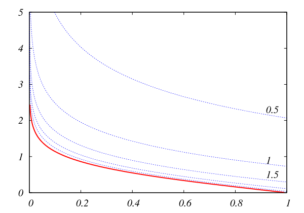
Viceversa, for any $\rho\geq\rho_{\rm c}(\delta)$ , we have $M^{*}(\delta,\rho)=\infty$ .

Figure 11 shows the location of the noise sensitivity boundary $\rho_{\rm c}(\delta)$ as well as the level lines of $M^{*}(\delta,\rho)$ for $\rho<\rho_{\rm c}(\delta)$ . Above $\rho_{\rm c}(\delta)$ the LASSO MSE is not uniformly bounded in terms of the measurement noise $\sigma^{2}$ . Other estimators (for instance one step of soft thresholding) can offer better stability guarantees in this region.

One remarkable fact is that the phase boundary $\rho=\rho_{\rm c}(\delta)$ coincides with the phase transition for $\ell_{0}-\ell_{1}$ equivalence derived earlier by Donoho [Don06] on the basis of random polytope geometry results by Affentranger-Schneider [AS92]. The same phase transition was further studied in a series of papers by Donoho, Tanner and coworkers [DT05, DT09], in connection with the noiseless estimation problem. For $\rho<\rho_{\rm c}$ estimating $x$ by $\ell_{1}$ -norm minimization returns the correct signal with high probability (over the choice of the random matrix $A$ ). For $\rho>\rho_{\rm c}(\delta)$ , $\ell_{1}$ -minimization fails.

Here this phase transition is derived from a completely different perspective as a special case of a stronger result. We indeed use a new method –the state evolution analysis of the AMP algorithm– which offers quantitative information about the noisy case as well, namely it allows to compute the value of $M^{*}(\delta,\rho)$ for $\rho<\rho_{\rm c}(\delta)$ . Within the present approach, the line $\rho_{\rm c}(\delta)$ admits a very simple expresson. In parametric form, it is given by

	$\displaystyle\delta$	$\displaystyle=$	$\displaystyle\frac{2\phi(\alpha)}{\alpha+2(\phi(\alpha)-\alpha\Phi(-\alpha))}\,,$		(6.22)
	$\displaystyle\rho$	$\displaystyle=$	$\displaystyle 1-\frac{\alpha\Phi(-\alpha)}{\phi(\alpha)}\,,$		(6.23)

where $\phi$ and $\Phi$ are the Gaussian density and Gaussian distribution function, and $\alpha\in[0,\infty)$ is the parameter. Indeed $\alpha$ has a simple and practically important interpretation as well. Recall that the AMP algorithm uses a sequence of thresholds $\theta_{t}=\alpha\widehat{\tau}_{t}$ , cf. Eqs. (5.6) and (5.7). How should the parameter $\alpha$ be fixed? A very simple prescription is obtained in the noiseless case. In order to achieve exact reconstruction for all $\rho<\rho_{\rm c}(\delta)$ for a given an undersampling ratio $\delta$ , $\alpha$ should be such that $(\delta,\rho_{\rm c}(\delta))=(\delta(\alpha),\rho(\alpha))$ with functions $\alpha\mapsto\delta(\alpha)$ , $\alpha\mapsto\rho(\alpha)$ defined as in Eq. (6.22), (6.23). In other words, this parametric expression yields each point of the phase boundary as a function of the threshold parameter used to achieve it via AMP.

6.7 On universality

The main results presented in this section, namely Theorems 6.1, 6.3 and 6.5, are proved for measurement matrices with i.i.d. Gaussian entries. As stressed above, it is expected that the same results hold for a much broader class of matrices. In particular, they should extend to matrices with i.i.d. or weakly correlated entries. For the sake of clarity, it is useful to put forward a formal conjecture, that generalizes Theorem 6.3.

Conjecture 6.6.

Let $\{x(n),w(n),A(n)\}_{n\in{\mathbb{N}}}$ be a converging sequence of instances with the entries of $A(n)$ i.i.d. with mean ${\mathbb{E}}\{A_{ij}\}=0$ , variance ${\mathbb{E}}\{A_{ij}^{2}\}=1/m$ and such that ${\mathbb{E}}\{A_{ij}^{6}\}\leq C/m$ for some fixed constant $C$ . Denote by $\widehat{x}(\lambda)$ the LASSO estimator for instance $(x(n),w(n),A(n))$ , with $\sigma^{2},\lambda>0$ , and let $\psi:{\mathbb{R}}\times{\mathbb{R}}\to{\mathbb{R}}$ be a pseudo-Lipschitz function. Then, almost surely

\displaystyle\lim_{n\to\infty}\frac{1}{n}\sum_{i=1}^{n}\psi\big(\widehat{x}_{i},x_{i}\big)={\mathbb{E}}\Big\{\psi\big(\eta(X_{0}+\tau_{*}Z;\theta_{*}),X_{0}\big)\Big\}\,,

(6.24)

where $Z\sim{\sf N}(0,1)$ is independent of $X_{0}\sim p_{0}$ , $\tau_{*}=\tau_{*}(\alpha(\lambda))$ and $\theta_{*}=\alpha(\lambda)\tau_{*}(\alpha(\lambda))$ are given by the same formulae holding for Gaussian matrices, cf. Section 6.3.

The conditions formulated in this conjecture are motivated by the universality result in [KM10b], that provides partial evidence towards this claim. Simulations (see for instance Fig. 10 and [BBM11]) strongly support this claim.

While proving Conjecture 6.6 is an outstanding mathematical challenge, many measurement models of interest do not fit the i.i.d. model. Does the theory developed in these section say anything about such measurements? Systematic numerical simulations [DMM10b, BBM11] reveal that, even for highly structured matrices, the same formula 6.24 is either surprisingly close to the actual empirical performances.

As an example, Fig. 12 presents the empirical mean square error for a partial Fourier measurement matrix $A$ , as a function of the regularization parameter $\lambda$ . The matrix is obtained by subsampling the rows of the $N\times N$ Fourier matrix $F$ , with entries $F_{ij}=e^{2\pi ij\sqrt{-1}}$ . More precisely we sample $n/2$ rows of $F$ with replacement, construct two rows of $A$ by taking real and imaginary part, and normalize the columns of the resulting matrix.

Figure 13 presents analogous results for the random demodulator matrix which is at the core of the analog-to-digital converter (ADC) of [TLD+10]. Schematically, this is obtained by normalizing the columns of $\widetilde{A}=HDF$ , with $F$ a Fourier matrix, $D$ a random diagonal matrix with $D_{ii}\in\{+1,-1\}$ uniformly at random, and $H$ an ‘accumulator’:

\displaystyle H=\left[\begin{array}[]{cccc}1111&&&\\ &1111&&\\ &&\cdots&\\ &&&1111\\ \end{array}\right]\,.

Both these examples show good agreement between the asymptotic prediction provided by Theorem 6.3 and the empirical mean square error. Such an agreement is surprising given that in both cases the measurement matrix is generated with a small amount of randomness, compared to a Gaussian matrix. For instance, the ADC matrix only requires $n$ random bits. Although statistically significant discrepancies can be observed (cf. for instance Fig. 13), the present approach provides quantitative predictions of great interest for design purposes. For a more systematic investigation, we refer to [BBM11].

6.8 Comparison with other analysis approaches

The analysis presented here is significantly different from more standard approaches. We derived an exact characterization for the high-dimensional limit of the LASSO estimation problem under the assumption of converging sequences of random sensing matrices.

Alternative approaches assume an appropriate ‘isometry’, or ‘incoherence’ condition to hold for $A$ . Under this condition upper bounds are proved for the mean square error. For instance Candes, Romberg and Tao [CRT06] prove that the mean square error is bounded by $C\sigma^{2}$ for some constant $C$ . Work by Candes and Tao [CT07] on the analogous Dantzig selector, upper bounds the mean square error by $C\sigma^{2}(k/n)\log n$ , with $k$ the number of non-zero entries of the signal $x$ .

These type of results are very robust but present two limitations: $(i)$ They do not allow to distinguish reconstruction methods that differ by a constant factor (e.g. two different values of $\lambda$ ); $(ii)$ The restricted isometry condition (or analogous ones) is quite restrictive. For instance, it holds for random matrices only under very strong sparsity assumptions. These restrictions are intrinsic to the worst-case point of view developed in [CRT06, CT07].

Guarantees have been proved for correct support recovery in [ZY06], under an incoherence assumption on $A$ . While support recovery is an interesting conceptualization for some applications (e.g. model selection), the metric considered in the present paper (mean square error) provides complementary information and is quite standard in many different fields.

Close to the spirit of the treatment presented here, [RFG09] derived expressions for the mean square error under the same model considered here. Similar results were presented recently in [KWT09, GBS09]. These papers argue that a sharp asymptotic characterization of the LASSO risk can provide valuable guidance in practical applications. Unfortunately, these results were non-rigorous and were obtained through the famously powerful ‘replica method’ from statistical physics [MM09]. The approach discussed here offers two advantages over these recent developments: $(i)$ It is completely rigorous, thus putting on a firmer basis this line of research; $(ii)$ It is algorithmic in that the LASSO mean square error is shown to be equivalent to the one achieved by a low-complexity message passing algorithm.

Finally, recently random models for the measurement matrix have been studied in [CP09, CP10b]. The approach developed in these papers allows to treat matrices that do not necessarily satisfy the restricted isometry property or similar conditions, and applies to a general class of random matrices $A$ with i.i.d. rows. On the other hand, the resulting bounds are not asymptotically sharp.

7 Generalizations

The single most important advantage of the point of view based on graphical models is that it offers a unified disciplined approach to exploit structural information on the signal $x$ . The use of such information can dramatically reduce the number of required compressed sensing measurements.

‘Model-based’ compressed sensing [BCDH10] provides a general framework for specifying such information. However, it focuses on ‘hard’ combinatorial information about the signal. Graphical models are instead a rich language for specifying ‘soft’ dependencies or constraints, and more complex models. These might include combinatorial constraints, but vastly generalize them. Also, graphical models come with an algorithmic arsenal that can be applied to leverage the potential of such more complex signal models.

Exploring such potential generalizations is –to a large extent– a future research program which is still in its infancy. Here we will only discuss a few examples.

7.1 Structured priors…

Block-sparsity is a simple example of combinatorial signal structure. We decompose the signal as $x=(x_{B(1)},$ $x_{B(2)},$ $\dots,$ $x_{B(\ell)})$ where $x_{B(i)}\in{\mathbb{R}}^{n/\ell}$ is a block for $\ell\in\{1,\dots,\ell\}$ . Only a fraction $\varepsilon\in(0,1)$ of the blocks is non-vanishing. This type of model naturally arises in many applications: for instance the case $\ell=n/2$ (blocks of size $2$ ) can model signals with complex-valued entries. Larger blocks can correspond to shared sparsity patterns among many vectors, or to clustered sparsity.

It is customary in this setting to replace the LASSO cost function with the following

\displaystyle{\cal C}^{{\rm Block}}_{A,y}(z)

\displaystyle\equiv\frac{1}{2}\|y-Az\|_{2}^{2}+\lambda\sum_{i=1}^{\ell}\|z_{B(i)}\|_{2}\,.

(7.1)

The block- $\ell_{2}$ regularization promotes block sparsity. Of course, the new regularization can be interpreted in terms of a new assumed prior that factorizes over blocks.

Figure 14 reproduces two possible graphical structures that encode the block-sparsity constraint. In the first case, this is modeled explicitly as a constraint over blocks of variable nodes, each block comprising $n/\ell$ variables. In the second case, blocks correspond explicitly to variables taking values in ${\mathbb{R}}^{n/\ell}$ . Each of these graphs dictates a somewhat different message passing algorithm.

An approximate message passing algorithm suitable for this case is developed in [DM10]. Its analysis allows to generalize $\ell_{0}-\ell_{1}$ phase transition curves reviewed in Section 6.6 to the block sparse case. This quantifies precisely the benefit of minimizing (7.1) over simple $\ell_{1}$ penalization.

As mentioned above, for a large class of signals sparsity is not uniform: some subsets of entries are sparser than others. Tanaka and Raymond [TR10], and Som, Potter and Schniter and [SSS10] studied the case of signals with multiple level of sparsity. The simplest example consists of a signal $x=(x_{B(1)},x_{B(2)})$ , where $x_{B(1)}\in{\mathbb{R}}^{n_{1}}$ , $x_{B(2)}\in{\mathbb{R}}^{n_{2}}$ , $n_{1}+n_{2}=n$ . Block $i\in\{1,2\}$ has a fraction $\varepsilon_{i}$ of non-zero entries, with $\varepsilon_{1}\neq\varepsilon_{2}$ . In the most complex case, one can consider a general factorized prior

\displaystyle p({\rm d}x)=\prod_{i=1}^{n}p_{i}({\rm d}x_{i})\,,

where each $i\in[n]$ has a different sparsity parameter $\varepsilon_{i}\in(0,1)$ , and $p_{i}\in{\cal F}_{\varepsilon_{i}}$ . In this case it is natural to use a weighted– $\ell_{1}$ regularization, i.e. to minimize

\displaystyle{\cal C}^{{\rm weight}}_{A,y}(z)

\displaystyle\equiv\frac{1}{2}\|y-Az\|_{2}^{2}+\lambda\sum_{i=1}^{n}w_{i}\,|z_{i}|\,,

(7.2)

for a suitable choice of the weights $w_{1},$ $\dots,$ $w_{n}\geq 0$ . The paper [TR10] studies the case $\lambda\to 0$ (equivalent to minimizing $\sum_{i}w_{i}|z_{i}|$ subject to $y=Az$ ), using non-rigorous statistical mechanics techniques that are equivalent to the state evolution approach presented here. Within a high-dimensional limit, it determines optimal tuning of the parameters $w_{i}$ , for given sparsities $\varepsilon_{i}$ . The paper [SSS10] follows instead the state evolution approach explained in the present chapter. The authors develop a suitable AMP iteration and compute the optimal thresholds to be used by the algorithm. These are in correspondence with the optimal weights $w_{i}$ mentioned above, and can be also interpreted within the minimax framework developed in the previous pages.

The graphical model framework is particularly convenient for exploiting prior information that is probabilistic in nature, see in particular [CHDB08, CICB10]. A prototypical example was studied by Schniter [Sch10] who considered the case in which the signal $x$ is generated by an Hidden Markov Model (HMM). As for the block-sparse model, this can be used to model signals in which the non-zero coefficients are clustered, although in this case one can accomodate greater stochastic variability of the cluster sizes.

In the simple case studied in detail in [Sch10], the underlying Markov chain has two states indexed by $s_{i}\in\{0,1\}$ , and

\displaystyle p({\rm d}x)=\sum_{s_{1},\dots,s_{n}}\Big\{\prod_{i=1}^{n}p({\rm d}x_{i}|s_{i})\cdot\prod_{i=1}^{n-1}p(s_{i+1}|s_{i})\,\cdot p_{1}(s_{1})\Big\}\,,

(7.3)

where $p(\,\cdot\,|0)$ and $p(\,\cdot\,|1)$ belong to two different sparsity classes ${\cal F}_{\varepsilon_{0}}$ , ${\cal F}_{\varepsilon_{1}}$ . For instance one can consider the case in which $\varepsilon_{0}=0$ and $\varepsilon_{1}=1$ , i.e. the support of $x$ coincides with the subset of coordinates such that $s_{i}=1$ .

Figure 15 reproduces the graphical structure associated with this type of models. This can be partitioned in two components: a bipartite graph corresponding to the compressed sensing measurements (upper part in Fig. 15) and a chain graph corresponding to the Hidden Markov Model structure of the prior (lower part in Fig. 15).

Reconstruction was performed in [Sch10] using a suitable generalization of AMP. Roughly speaking, inference is performed in the upper half of the graph using AMP and in the lower part using the standard forward-backward algorithm. Information is exchanged across the two component in a way that is very similar to what happens in turbo codes [RU08].

The example of HMM priors clarifies the usefulness of the graphical model structure in eliciting tractable substructures in the probabilistic model and hence leading to natural iterative algorithms. For an HMM prior, inference can be performed efficiently because the underlying graph is a simple chain.

A broader class of priors for which inference is tractable is provided by Markov-tree distributions [SPS10]. These are graphical models that factors according to a tree graph (i.e. a graph without loops). A cartoon of the resulting compressed sensing model is reproduced in Figure 16.

The case of tree-structured priors is particularly relevant in imaging applications. Wavelet coefficients of natural images are sparse (an important motivating remark for compressed sensing) and non-zero entries tend to be localized along edges in the image. As a consequence, they cluster in subtrees of the tree of wavelet coefficients. A Markov-tree prior can capture well this structure.

Again, reconstruction is performed exactly on the tree-structured prior (this can be done efficiently using belief propagation), while AMP is used to do inference over the compressed sensing measurements (the upper part of Figure 16).

7.2 Sparse sensing matrices

Throughout this review we focused for simplicity on dense measurement matrices $A$ . Several of the mathematical results presented in the previous sections do indeed hold for dense matrices with i.i.d. components. Graphical models ideas are on the other hand particularly useful for sparse measurements.

Sparse sensing matrices present several advantages, most remarkably lower measurement and reconstruction complexities [BGI+08]. While sparse constructions are not suitable for all applications, they appear a promising solution for networking applications, most notably in network traffic monitoring [CM04, LMP+08b].

In an over-simplified example, one would like to monitor the sizes of $n$ packet flows at a router. It is a recurring empirical observation that most of the flows consist of a few packets, while most of the traffic is accounted for by a few flows. Denoting by $x_{1}$ , $x_{2}$ , … $x_{n}$ the flow sizes (as measured, for instance, by the number of packets belonging to the flow), it is desirable to maintain a small sketch of the vector $x=(x_{1},\dots,x_{n})$ .

Figure 17 describes a simple approach: flow $i$ hashes into a small number –say $k$ – of memory spaces, ${\partial i}=\{a_{1}(i),\dots,a_{k}(i)\}\subseteq[m]$ . Each time a new packet arrives for flow $i$ , the counters in ${\partial i}$ are incremented. If we let $y=(y_{1},\dots,y_{m})$ be the contents of the counters, we have

\displaystyle y=Ax\,,

(7.4)

where $x\geq 0$ and $A$ is a matrix with i.i.d. columns with $k$ entries per column equal to $1$ and all the other entries equal to $0$ . While this simple scheme requires unpractically deep counters (the entries of $y$ can be large), [LMP+08b] showed how to overcome this problem by using a multi-layer graph.

Numerous algorithms were developed for compressed sensing reconstruction with sparse measurement matrices [CM04, XH07, BGI+08, Ind08]. Most of these algorithms are based on greedy methods, which are essentially of message passing type. Graphical models ideas can be used to construct such algorithms in a very natural way. For instance, the algorithm of [LMP+08b] (see also [LMP07, LMP08a, CSW10] for further analysis of the same algorithm) is closely related to the ideas presented in the rest of this chapter. It uses messages $x^{t}_{i\to a}$ (from variable nodes to function nodes) and $r_{a\to i}^{t}$ (from function nodes to variable nodes). These are updated according to

	$\displaystyle r^{t}_{a\to i}$	$\displaystyle=$	$\displaystyle y_{a}-\sum_{j\in{\partial a}\setminus i}x_{j\to a}^{t}\,,$		(7.5)
	$\displaystyle x^{t+1}_{i\to a}$	$\displaystyle=$	$\displaystyle\left\{\begin{array}[]{ll}\min\big\{r^{t}_{b\to i}:\;\;b\in{\partial i}\setminus a\big\}&\mbox{at even iterations $t$,}\\ \max\big\{r^{t}_{b\to i}:\;\;b\in{\partial i}\setminus a\big\}&\mbox{at odd iterations $t$,}\end{array}\right.$

where ${\partial a}$ denotes the set of neighbors of node $a$ in the factor graph. These updates are very similar to Eqs. (5.11), (5.12) introduced earlier in our derivation of AMP.

7.3 Matrix completion

‘Matrix completion’ is the task of inferring an (approximately) low rank matrix from observations on a small subset of its entries. This problem has attracted considerable interest offer the last two years due to its relevance in a number of applied domains (collaborative filtering, positioning, computer vision, etc.).

Significant progress has been achieved on the theoretical side. The reconstruction question has been addressed in analogy with compressed sensing in [CR09, CP10a, Gro09, NW09], while an alternative approach based on greedy methods was developed in [KMO10a, KMO10b, KM10a]. While the present chapter does not treat matrix completion in any detail, it is interesting to mention that graphical models ideas can be useful in this context as well.

Let $M\in{\mathbb{R}}^{m\times n}$ be the matrix to be reconstructed, and assume that a subset $E\subseteq[m]\times[n]$ of its entries is observed. It is natural to try to accomplish this task by minimizing the $\ell_{2}$ distance on observed entries. For $X\in{\mathbb{R}}^{m\times r}$ , $Y\in{\mathbb{R}}^{n\times r}$ , we introduce therefore the cost function

\displaystyle{\cal C}(X,Y)=\frac{1}{2}\,\|{\cal P}_{E}(M-XY^{T})\|_{F}^{2}

(7.9)

where ${\cal P}_{E}$ is the projector that sets to zero the entries outside $E$ (i.e. ${\cal P}_{E}(L)_{ij}=L_{ij}$ if $(i,j)\in E$ and ${\cal P}_{E}(L)_{ij}=0$ otherwise). If we denote the rows of $X$ as $x_{1},\dots,x_{m}\in{\mathbb{R}}^{r}$ and the rows in $Y$ as $y_{1},\dots,y_{n}\in{\mathbb{R}}^{r}$ , the above cost function can be rewritten as

\displaystyle{\cal C}(X,Y)=\frac{1}{2}\sum_{(i,j)\in E}\big(M_{ij}-\langle x_{i},y_{j}\rangle\big)^{2}\,,

(7.10)

with $\langle\,\cdot\,,\,\cdot,\rangle$ the standard scalar product on ${\mathbb{R}}^{r}$ . This cost function factors accordingly the bipartite graph $G$ with vertex sets $V_{1}=[m]$ and $V_{2}=[n]$ and edge set $E$ . The cost decomposes as a sum of pairwise terms associated with the edges of $G$ .

Figure 18 reproduces the graph $G$ that is associated to the cost function ${\cal C}(X,Y)$ . It is remarkable some properties of the reconstruction problem can be ‘read’ from the graph. For instance, in the simple case $r=1$ , the matrix $M$ can be reconstructed if and only if $G$ is connected (banning for degenerate cases) [KMO08]. For higher values of the rank $r$ , rigidity of the graph is related to uniqueness of the solution of the reconstruction problem [SC09]. Finally, message passing algorithms for this problem were studied in [KYP10, KM10a].

7.4 General regressions

The basic reconstruction method discussed in this review is the regularized least-squares regression defined in Eq. (2.8), also known as the LASSO. While this is by far the most interesting setting for signal processing applications, for a number of statistical learning problems, the linear model (1.1) is not appropriate. Generalized linear models provide a flexible framework to extend the ideas discussed here.

An important example is logistic regression, which is particularly suited for the case in which the measurements $y_{1},$ $\dots$ $y_{m}$ are $0$ – $1$ valued. Within logistic regression, these are modeled as independent Bernoulli random variables with

\displaystyle p(y_{a}=1|x)=\frac{e^{A_{a}^{T}x}}{1+e^{A_{a}^{T}x}}\,,

(7.11)

with $A_{a}$ a vector of ‘features’ that characterizes the $a$ -th experiment. The objective is to learn the vector $x$ of coefficients that encodes the relevance of each feature. A possible approach consists in minimizing the regularized (negative) log-likelihood, that is

\displaystyle{\cal C}^{{\rm LogReg}}_{A,y}(z)

\displaystyle\equiv-\sum_{a=1}^{m}y_{a}(A_{a}^{T}z)+\sum_{a=1}^{m}\log\big(1+e^{A_{a}^{T}z}\big)+\lambda\|z\|_{1}\,,

(7.12)

The papers [Ran10, BM10] develops approximate message passing algorithms for solving optimization problems of this type.

Acknowledgements

It is a pleasure to thank Mohsen Bayati, Jose Bento, David Donoho and Arian Maleki, with whom this research has been developed. This work was partially supported by a Terman fellowship, the NSF CAREER award CCF-0743978 and the NSF grant DMS-0806211.

References

[AJ07] G. Andrew and G. Jianfeng, Scalable training of $l^{1}$ -regularized log-linear models, Proceedings of the 24th international conference on Machine learning, 2007, pp. 33–40.
[AS92] R. Affentranger and R. Schneider, Random projections of regular simplices, Discr. and Comput. Geometry 7 (1992), 219–226.
[AS03] D. Aldous and J. M. Steele, The Objective Method: Probabilistic Combinatorial Optimization and Local Weak Convergence, Probability on discrete structures (H. Kesten, ed.), Springer Verlag, 2003, pp. 1–72.
[BBM11] M. Bayati, J. Bento, and A. Montanari, Universality in sparse reconstruction: A comparison between theories and empirical results, in preparation, 2011.
[BCDH10] R. G. Baraniuk, V. Cevher, M. F. Duarte, and C. Hegde, Model-Based Compressive Sensing, IEEE Trans. on Inform. Theory 56 (2010), 1982–2001.
[BGI⁺08] R. Berinde, A. C. Gilbert, P. Indyk, H. Karloff, and M. J. Strauss, Combining Geometry and Combinatorics: A Unified Approach to Sparse Signal Recovery, 46th Annual Allerton Conference (Monticello, IL), September 2008.
[Bil95] P. Billingsley, Probability and Measure, Wiley, USA, 1995.
[BM10] M. Bayati and A. Montanari, Approximate message passing algorithms for generalized linear models, in preparation, 2010.
[BM11] , The dynamics of message passing on dense graphs, with applications to compressed sensing, IEEE Trans. on Inform. Theory (2011), accepted, http://arxiv.org/pdf/1001.3448.
[CD95] S.S. Chen and D.L. Donoho, Examples of basis pursuit, Proceedings of Wavelet Applications in Signal and Image Processing III (San Diego, CA), 1995.
[Cev08] V. Cevher, Learning with compressible priors, Neural Information Processing Systems (Vancouver), December 2008.
[CHDB08] V. Cevher, C. Hegde, M. F. Duarte, and R. G. Baraniuk, Sparse Signal Recovery Using Markov Random Fields, Neural Information Processing Systems (Vancouver), December 2008.
[CICB10] V. Cevher, P. Indyk, L. Carin, and R.G. Baraniuk, Sparse Signal Recovery and Acquisition with Graphical Models, IEEE Signal Processing Magazine 27 (2010), 92–103.
[CM04] G. Cormode and S. Muthukrishnan, Improved data streams summaries: The count-min sketch and its aplications, Latin (Buenos Aires), 2004, pp. 29–38.
[CP09] E. J. Candès and Y. Plan, Near-ideal model selection by $\ell_{1}$ minimization, Ann. Statist. 37 (2009), 2145–2177.
[CP10a] , Matrix completion with noise, Proceedings of the IEEE 98 (2010), 925–936.
[CP10b] , A probabilistic and ripless theory of compressed sensing, arXiv:1011.3854, November 2010.
[CR09] E. J. Candès and B. Recht, Exact matrix completion via convex optimization, Found. of Comput. Math. 9 (2009), 717–772.
[CRT06] E. Candes, J. K. Romberg, and T. Tao, Stable signal recovery from incomplete and inaccurate measurements, Communications on Pure and Applied Mathematics 59 (2006), 1207–1223.
[CSW10] V. Chandar, D. Shah, and G. W. Wornell, A simple message-passing algorithm for compressed sensing, Proceedings of IEEE International Symposium on Inform. Theory (ISIT) (Austin), 2010.
[CT07] E. Candes and T. Tao, The Dantzig selector: statistical estimation when p is much larger than n, Annals of Statistics 35 (2007), 2313–2351.
[DJ94a] D. L. Donoho and I. M. Johnstone, Ideal spatial adaptation via wavelet shrinkage, Biometrika 81 (1994), 425–455.
[DJ94b] , Minimax risk over $l_{p}$ balls, Prob. Th. and Rel. Fields 99 (1994), 277–303.
[DJHS92] D.L. Donoho, I.M. Johnstone, J.C. Hoch, and A.S. Stern, Maximum entropy and the nearly black object, Journal of the Royal Statistical Society, Series B (Methodological) 54 (1992), no. 1, 41–81.
[DM10] D. Donoho and A. Montanari, Approximate message passing for reconstruction of block-sparse signals, in preparation, 2010.
[DMM09] D. L. Donoho, A. Maleki, and A. Montanari, Message Passing Algorithms for Compressed Sensing, Proceedings of the National Academy of Sciences 106 (2009), 18914–18919.
[DMM10a] , Message Passing Algorithms for Compressed Sensing: I. Motivation and Construction, Proceedings of IEEE Inform. Theory Workshop (Cairo), 2010.
[DMM10b] D.L. Donoho, A. Maleki, and A. Montanari, The Noise Sensitivity Phase Transition in Compressed Sensing, http://arxiv.org/abs/1004.1218, 2010.
[Don06] D. Donoho, High-dimensional centrally symmetric polytopes with neighborliness proportional to dimension, Discr. and Comput. Geometry 35 (2006), 617–652.
[DT05] D. L. Donoho and J. Tanner, Neighborliness of randomly-projected simplices in high dimensions, Proceedings of the National Academy of Sciences 102 (2005), no. 27, 9452–9457.
[DT09] , Counting faces of randomly projected polytopes when the projection radically lowers dimension, Journal of American Mathematical Society 22 (2009), 1–53.
[FN03] M.A.T. Figueiredo and R.D. Nowak, An EM algorithm for wavelet-based image restoration, IEEE Trans. on Image Proc. 12 (2003), 906–916.
[GB10] M. Grant and S. Boyd, CVX: Matlab software for disciplined convex programming, version 1.21, http://cvxr.com/cvx, May 2010.
[GBS09] D. Guo, D. Baron, and S. Shamai, A single-letter characterization of optimal noisy compressed sensing, 47th Annual Allerton Conference (Monticello, IL), September 2009.
[GK07] D. Gamarnik and D. Katz, Correlation decay and deterministic FPTAS for counting list-colorings of a graph, 18th annual ACM-SIAM Symposium On Discrete Algorithm (New Orleans), 2007, pp. 1245–1254.
[Gro09] D. Gross, Recovering low-rank matrices from few coefficients in any basis, arXiv:0910.1879v2, 2009.
[GV05] D. Guo and S. Verdu, Randomly Spread CDMA: Asymptotics via Statistical Physics, IEEE Trans. on Inform. Theory 51 (2005), 1982–2010.
[HTF03] T. Hastie, R. Tibshirani, and J. Friedman, The Elements of Statistical Learning, Springer-Verlag, New York, 2003.
[Ind08] P. Indyk, Explicit constructions for compressed sensing of sparse signals, 19th annual ACM-SIAM Symposium On Discrete Algorithm (San Francisco), January 2008.
[Joh02] I. Johnstone, Function Estimation and Gaussian Sequence Models, Draft of a book, available at http://www-stat.stanford.edu/ $\sim$ imj/based.pdf, 2002.
[Jor98] M. Jordan (ed.), Learning in graphical models, MIT Press, Boston, 1998.
[JXC08] S. Ji, Y. Xue, and L. Carin, Bayesian Compressive Sensing, IEEE Trans. on Signal Proc. 56 (2008), 2346–2356.
[KF09] D. Koller and N. Friedman, Probabilistic Graphical Models, MIT Press, Cambridge, 2009.
[KM10a] R. H. Keshavan and A. Montanari, Fast algorithms for matrix completion, In preparation, 2010.
[KM10b] S. Korada and A. Montanari, Applications of Lindeberg Principle in Communications and Statistical Learning, http://arxiv.org/abs/1004.0557, 2010.
[KMO08] R. H. Keshavan, A. Montanari, and S. Oh, Learning low rank matrices from $O(n)$ entries, Proc. of the Allerton Conf. on Commun., Control and Computing, September 2008, arXiv:0812.2599.
[KMO10a] , Matrix completion from a few entries, IEEE Trans. on Inform. Theory 56 (2010), 2980–2998.
[KMO10b] , Matrix completion from noisy entries, J. Mach. Learn. Res. 11 (2010), 2057–2078.
[KWT09] Y. Kabashima, T. Wadayama, and T. Tanaka, A typical reconstruction limit for compressed sensing based on lp-norm minimization, J.Stat. Mech. (2009), L09003.
[KYP10] B.-H. Kim, A. Yedla, and H. D. Pfister, Imp: A message-passing algorithmfor matrix completion, Proc. 6th International Symposium on Turbo Codes, September 2010, arXiv:1007.0481.
[LC98] E.L. Lehmann and G. Casella, Theory of Point Estimation, Springer-Verlag, New York, 1998.
[Led01] M. Ledoux, The concentration of measure phenomenon, American Mathematical Society, Berlin, 2001.
[LMP07] Y. Lu, A. Montanari, and B. Prabhakar, Detailed Network Measurements Using Sparse Graph Counters: The Theory, 45th Annual Allerton Conference (Monticello, IL), September 2007.
[LMP08a] , Counter Braids: Asymptotic optimality of the message passing decoding algorithm, 46th Annual Allerton Conference (Monticello, IL), September 2008.
[LMP⁺08b] Y. Lu, A. Montanari, B. Prabhakar, S. Dharmapurikar, and A. Kabbani, Counter braids: a novel counter architecture for per-flow measurement, SIGMETRICS 2010, 2008.
[MD10] A. Maleki and D. L. Donoho, Optimally tuned iterative thresholding algorithm for compressed sensing, IEEE Journal of Selected Topics in Signal Processing 4 (2010), 330–341.
[MM09] M. Mézard and A. Montanari, Information, Physics and Computation, Oxford University Press, Oxford, 2009.
[Mon08] A. Montanari, Estimating random variables from random sparse observations, Eur. Trans. on Telecom. 19 (2008), 385–403.
[MPV87] M. Mézard, G. Parisi, and M. A. Virasoro, Spin glass theory and beyond, World Scientific, Singapore, 1987.
[MR07] C. Moallemi and B. Van Roy, Convergence of the min-sum algorithm for convex optimization, 45th Annual Allerton Conference (Monticello, IL), September 2007.
[MT06] A. Montanari and D. Tse, Analysis of belief propagation for non-linear problems: the example of CDMA (or: how to prove Tanaka’s formula), Proceedings of IEEE Inform. Theory Workshop (Punta de l’Este, Uruguay), 2006.
[NW09] S. Negahban and M. J. Wainwright, Estimation of (near) low-rank matrices with noise and high-dimensional scaling, arXiv:0912.5100, 2009.
[Ons36] L. Onsager, Electric Moments of Molecules in Liquids, J. Amer. Chem. Soc. 58 (1936), 1486–1493.
[Pea88] J. Pearl, Probabilistic reasoning in intelligent systems: networks of plausible inference, Morgan Kaufmann, San Francisco, 1988.
[Ran10] S. Rangan, Generalized approximate message passing for estimation with random linear mixing, arXiv:1010.5141, 2010.
[RFG09] S. Rangan, A. K. Fletcher, and V. K. Goyal, Asymptotic analysis of map estimation via the replica method and applications to compressed sensing, PUT NIPS REF, 2009.
[RU08] T.J. Richardson and R. Urbanke, Modern Coding Theory, Cambridge University Press, Cambridge, 2008.
[SBB10] S. Sarvotham, D. Baron, and R. Baraniuk, Bayesian Compressive Sensing via Belief Propagation, IEEE Trans. on Signal Processing 58 (2010), 269–280.
[SC09] A. Singer and M. Cucuringu, Uniqueness of low-rank matrix completion by rigidity theory, arXiv:0902.3846, January 2009.
[Sch10] P. Schniter, Turbo Reconstruction of Structured Sparse Signals, Proceedings of the Conference on Information Sciences and Systems (Princeton), 2010.
[SPS10] S. Som, L. C. Potter, and P. Schniter, Compressive Imaging using Approximate Message Passing and a Markov-Tree Prior, Proc. Asilomar Conf. on Signals, Systems, and Computers, November 2010.
[SSS10] L.C. Potter S. Som and P. Schniter, On Approximate Message Passing for Reconstruction of Non-Uniformly Sparse Signals, Proceedings of the National Aereospace and Electronics Conference (Dayton, OH), 2010.
[Tan02] T. Tanaka, A Statistical-Mechanics Approach to Large-System Analysis of CDMA Multiuser Detectors, IEEE Trans. on Inform. Theory 48 (2002), 2888–2910.
[TAP77] D. J. Thouless, P. W. Anderson, and R. G. Palmer, Solution of ‘Solvable model of a spin glass’, Phil. Mag. 35 (1977), 593–601.
[Tib96] R. Tibshirani, Regression shrinkage and selection with the lasso, J. Royal. Statist. Soc B 58 (1996), 267–288.
[TLD⁺10] J. A. Tropp, J. N. Laska, M. F. Duarte, J. K. Romberg, and R. G. Baraniuk, Beyond Nyquist: Efficient Sampling of Sparse Bandlimited Signals, IEEE Trans. on Inform. Theory 56 (2010), 520–544.
[TR10] T. Tanaka and J. Raymond, Optimal incorporation of sparsity information bt weighted $L_{1}$ optimization, Proceedings of IEEE International Symposium on Inform. Theory (ISIT) (Austin), 2010.
[vdV00] A.W. van der Vaart, Asymptotic Statistics, Cambridge University Press, Cambridge, 2000.
[Wei05] D. Weitz, Combinatorial criteria for uniqueness of Gibbs measures, Rand. Struct. Alg. 27 (2005), 445475.
[Wil91] D. Williams, Probability with Martingales, Cambridge University Press, Cambridge, 1991.
[WJ08] M. J. Wainwright and M. I. Jordan, Graphical Models, Exponential Families, and Variational Inference, Foundations and Trends in Machine Learning 1 (2008).
[XH07] W. Xu and B. Hassibi, Efficient Compressive Sensing with Deterministic Guarantees Using Expander Graphs, Proceedings of IEEE Inform. Theory Workshop (Tahoe City, CA), 2007.
[ZY06] P. Zhao and B. Yu, On model selection consistency of Lasso, The Journal of Machine Learning Research 7 (2006), 2541–2563.