Regge Field Theory in zero transverse dimensions:
loops versus ”net” diagrams
Thanks: Email: sergeyb@ariel.ac.il
Abstract
Toy models of interacting Pomerons with triple and quaternary Pomeron vertices in zero transverse dimension are investigated. Numerical solutions for eigenvalues and eigenfunctions of the corresponding Hamiltonians are obtained, providing the quantum solution for the scattering amplitude in both models. The equations of motion for the Lagrangians of the theories are also considered and the classical solutions of the equations are found. Full two-point Green functions (”effective” Pomeron propagator) and amplitude of diffractive dissociation process are calculated in the framework of RFT-0 approach. The importance of the loops contribution in the amplitude at different values of the model parameters is discussed as well as the difference between the models with and without quaternary Pomeron vertex.
1 Introduction
The complete understanding of the high energy scattering processes is impossible without the calculation of the contributions of the different unitarization corrections to the amplitude. In the QCD Pomeron framework, [1, 2, 3], these corrections are arose due the self Pomeron interactions via the triple Pomeron interactions vertices [4, 5]. These self Pomeron interactions lead to the very complicated picture of the amplitude’s evolution with rapidity, see for example [6, 7, 8, 9, 10].
There are few main approaches which claim that they properly describe the Pomeron self interactions. The first one is presented as a chain of the evolution equations with Balitsky-Kovchegov (BK) equation as a main field equation of the hierarchy, [11]. The BK equation may be formulated in the framework of the Color Glass Condensate Approach (CGK), [10], and may be properly analyzed in the terms of s-channel interacting color dipoles, [12]. This equation correctly describes the interaction of two non identical objects, for example such interactions as DIS on nuclei, see [13, 14, 15, 16, 17, 18, 19, 20]. Another approach is the QCD Reggeon Field Theory (RFT-QCD), which is formulated in the momentum space and based on the standard diagrammatic calculus, [6, 7, 8, 9, 21, 22, 23]. In this approach the BK equation describes a resummation of the ”fan” diagrams of the type depicted in Fig.1a with only Pomerons merging vertices considered.
Usual BK equation, describing ”fan” diagrams, does not include Pomeron’s splitting vertex. Therefore, the next natural step toward the unitarization of the amplitude is a symmetrical consideration of the scattering process with both vertices included. In this case the splitting vertex may be accounted differently in two different approximations. In the first approach the semi-classical problem of the interest is considered and there the sum of the diagrams depicted in Fig.1b is calculated, neglecting Pomeron loops contribution into amplitude. The second approach is concentrated on the solution of the full quantum problem basing on some effective high-energy QCD inspired models, accounting diagrams of Fig.1c type, see for example [24]. So far several attempts of the calculations were done in both directions, on the basis of QCD-RFT theory, [21, 22, 23] and in the framework of CGC and dipole model, [25]. The NLO and one-loop contribution into the amplitude also were calculated , see for example [26, 27], but the full solution still seems very far from it’s completeness. In this situation it is very natural to consider much simpler zero transverse dimensional model, in hope that some important properties of solutions of this model will be faced in QCD as well.
The RFT-0 (Reggeon Field Theory in zero transverse dimensions) model is attracted much interest during few last years, see [31]. The approach was formulated and studied a long time ago, even before the QCD era, see [28, 29, 30]. The interest to the approach is due very attractive properties of the model. First of all, RFT-0 is solvable at different parameters of the model. This possibility to find full solution for the different regimes of the theory is an important feature of the model, since we hope that we will understand more about RFT-QCD if we will have full and semi-classical solutions for RFT-0, see examples in [32, 33, 34]. Therefore, the second important fact about the RFT-0 is that in this theory we can find both classical and quantum solutions for the amplitude that provides us with the information about the relative contribution of the loops to the amplitude. The possibility to consider in RFT-0 different types of the Pomeron vertices is an another property of the RFT-0 which is very useful and which could clarify the situation in QCD.
In the paper we consider two RFT-0 models, in the second one together with usual triple Pomeron vertex we also include the quaternary Pomeron vertex. The paper is organized as follows. In the second section we consider the RFT-0 model with only triple Pomeron vertex. In two subsections of the section we introduce an whole machinery of the problem for the both quantum and classical solutions. In the following subsections we present the results of our calculations for the amplitude at different parameters of the model as well as the results for the two point Green’s function (”effective” Pomeron propagator ) of the theory. In the Sec.3 we solve the same problems for the RFT-0 theory with the quaternary Pomeron vertex included. The next section, Sec.4, is dedicated to the possible application of the solution to the problem of diffractive dissociation. The Sec.6 presents a summary of the results of the calculations and the last section, Sec.7, is the conclusion of our paper.
2 Solution of RFT in zero transverse dimension with only triple Pomeron coupling
In this paper we investigate the one-dimensional problem of the interacting Pomerons described by Lagrangian, which in the terms of Gribov fields has the following form:
| (1) |
where is the intercept of the bare Gribov field, is the triple field interactions vertex and differentiation means differentiation on rapidity (y) variable, which is only the variable of the problem. Introducing the Pomeron fields, and we rewrite the Lagrangian in the form of real coupling:
| (2) |
The field q and p may be understood now in the terms of the Pomeron creation and Pomeron annihilation operators :
| (3) |
The Hamiltonian of the problem in the terms of the operators q and p has the following form
| (4) |
being the second order differential operator:
| (5) |
The full, quantum solution of the theory will coincide, therefore, with the solution of the quantum mechanics problem with the Hamiltonian given by Eq.5:
| (6) |
where the function
| (7) |
is the full quantum amplitude of the process of the scattering of two particles. Here and denote eigenvalues and eigenfunctions of the operator Eq. 5, and are the normalized projections coefficients of the eigenfunctions on the value of at .
The classical solution of the theory, i.e. the solution with only ”tree” diagrams without loops also may be obtained in the given framework. It is simply the solution of equations of motion for the Lagrangian given by Eq. 2

2.1 The quantum solution of the model
An approximate solution of the Eq.6 was found many years ago, see [28, 29, 30]. Analytical solutions of the Eq.6 at large value of the ratio for ground state and first exited state were considered at the same time as well. Nevertheless, the spectrum of the theory and eigenfunctions for next exited states at large value of as well as the solutions for arbitrary values of were not obtained. Therefore, we want to define the procedure for the numerical calculations of the spectrum of the theory and corresponding eigenfunctions for the cases of the strong triple Pomeron coupling (small ) and week coupling (large ) as well. In the following we will be more interesting in the case of the small triple coupling as the case which is mostly correspond to the real perturbative QCD situation. So, we need to solve the second order differential equation (see more detailed in [29]):
| (8) |
with the initial and boundary conditions on the function :
| (11) | |||||
where form of depends on the particularly considered physical problem. Now it is constructive to make a transformation of the eigenfunctions:
| (12) |
In this case the term which is proportional to the first derivative over q is eliminated leading to hermitian Hamiltonian for the problem. After this transformation we obtain a Shredinger type eigenvalue equation:
| (13) |
with the following boundary conditions on the function :
| (15) | |||||
Our problem of interest is the scattering of two particles, therefore we define initial condition for the in the eikonal form (see more in [29]) :
| (16) |
here is a value of the source for the Pomeron field at zero rapidity. The function results the evolution of interacting Pomeron fields for the value of the Pomeron-external particle vertex equal to at zero rapidity, till the value of the single Pomeron field equal to at rapidity y.
The last ingredients of the theory are projection coefficients of the eigenfunctions of the solution on the initial state I(q). Having in mind, that our eigenfunctions are orthogonal on interval of q from to with weight function :
| (17) |
we obtain for :
| (18) |
where the weight function has the following form (see [29] and also [Heun]):
| (19) |
The numerical solution of Eq.13 with the boundary conditions given by Eq.15 is the solution for the eigenvalues and eigenfunctions of the second order differential equation with two boundary value conditions. These solutions for eigenfunctions and eigenvalues may be found for each values of and , i.e. for the different values of parameter . The obtained values of eigenfunctions and eigenfunctions allow to complete the calculation of the full quantum scattering amplitude and , therefore, solve our problem. So, considering the scattering of two particles , where the vertex of interaction of the first particle with Pomeron is equal and the vertex of interaction of the second particle with Pomeron is equal , we define the full , quantum solution for the scattering amplitude at given rapidity y as
| (20) |
with the given by Eq. 18 for the known values of eigenfunctions, see Fig.1c. The solution for the amplitude, Eq. 20, does not depend from which value of Pomeron field, or , the evolution begins. If we consider the evolution of the Pomeron from to we will obtain the same answer for the amplitude, as for the case of evolution from to .
2.2 The classical solution of the model
In order to see the role of the Pomeron loops in the scattering amplitude it is important to calculate the classical solution of our problem, given by the ”net” diagrams of Fig.1b. The comparison between two solutions will show a relative weight of the loops in the scattering amplitude and, therefore, an applicability of the classical solution at given values of the theory parameters. The required classical solution we obtain solving equations of motion for the Lagrangian given by Eq.2 with the sources of Pomeron fields at zero rapidity and final rapidity of the process Y:
| (21) |
where are the sources of the Pomeron fields. The equations of the motion for the fields p and q are the following:
| (25) | |||||
This system of equations is another example of two value boundary problem for the system of first order differential equations, and may be also solved for different values of parameters . The solutions of the system Eq.25 at given value of final rapidity Y and given values of parameters we will denote by . With the solution the ”net”, classical amplitude , represented by diagrams Fig.1b, is defined by standard way as:
| (26) |
where
| (27) |
The amplitude Eq.26 describes the eikonalized interactions of ”net” diagrams and for symmetric boundary conditions, , the amplitude is invariant under the duality transformations:
| (28) |
The interesting feature of the classical solution of the system defined by the Lagrangian Eq.21 is that starting from some critical rapidity the solution of equation of motion is not unique for . From the rapidity there are at least three classical trajectories which locally minimize the action and with increasing of the rapidities the number of the trajectories is growing. Each from them provides the local minimum of the action and the amplitude of the theory, therefore, must be rewritten in the following form:
| (29) |
where is the quantum weight of the corresponding classical trajectories. In the following consideration these weights we take equal 1 or -1, depending on the type of trajectory, see more detailed consideration of this problem in [30].
In our calculations of the classical amplitude for the symmetrical case , we always will use three solutions of the equations of motion. The first one, , is the symmetrical in the sence of Eq.28, which trajectory will be similar to the trajectory number 1 in the Fig.2. Another two dominant solutions, which we use in the calculations and which arise from some rapidity , are the solutions for the trajectories similar to the trajectories 2 and 3 in the Fig.2. Separately each of them is not symmetrical in the sense of the symmetry transformation given by the Eq.28, but instead, under the duality transformation of rapidity given by the Eq.28, there is a pair symmetry of these two solutions
| (30) |
It is interesting to note, that asymptotic behavior of these two classical solutions is well known, each of them may be described by ”fan” diagram amplitude of Fig.1a, see [29], and being the dominant contributions these solutions lead to the ”fan” dominance effect, see [32].
The final solution of our problem in the classical approximation we can write with the help of these three particular solutions as
| (31) |
which is symmetrical in respect to the duality transformation Eq.28. In our plots for the symmetrical interactions, , the classical solution will be always presented by amplitude of Eq.31, which contains three parts beginning from critical rapidity , and only one part, symmetrical solution, at rapidities smaller than . In the asymmetrical case the symmetry is broken initially, and, therefore, only one ”fan” configuration survives in the classical solution.

It is important to underline, that this picture for classical solution holds for each from the considered models, for RFT-0 with triple Pomeron vertex only and for RFT-0 model with both triple and quaternary vertexes.
2.3 Parameters of the model
First of all, we define the range and value of parameters for which the calculations were done in both cases, quantum and classical. We calculated quantum and classical amplitudes, and , for the following value of :
| (32) |
The reason of the main attention on this value of is very simple. The coupling constant in RFT-0 may be defined as and at we have, therefore, . This value for the coupling constant is reasonable also in QCD that provides the possibility of some analogies between two theories. The value of the external sources we take as follow
- •
symmetrical case:
(33) - •
non-symmetrical case:
(34)
As an example of the case of the strong coupling , i.e. large value of the triple vertex, we also will present the quantum solution for the symmetrical case of interaction at
| (35) |
Now it is instructive to consider the spectrum of the RFT-0 theory at different . The Table1 presents the found eigenvalues of the theory, for as well as for and for .
| 0.0546 | 0.292 | 0.609 | 0.997 | 1.447 | 1.95 | 2.503 | 3.103 | 3.745 | 4.427 | |
|---|---|---|---|---|---|---|---|---|---|---|
| 0.00217 | 0.142 | 0.297 | 0.507 | 0.759 | 1.047 | 1.37 | 1.724 | 2.108 | 2.579 | |
| 0.144 | 0.178 | 0.276 | 0.386 | 0.519 | 0.671 | 0.841 | 1.03 | 1.228 |
The asymptotic behavior of the amplitude is clearly seen from the Fig.3 which represents the behavior of the ground state as a function of .

Being important at small rapidity, all exited states, i.e. states with eigenvalues , at larger rapidities are decreasing very rapidly to zero. Therefore, at asymptotically large rapidity only the ground state survives, which nonzero origin is due the tunneling effect of the order which arises between the Coulomb and harmonic wells of the potential of the Eq.13, see [28, 29, 30]. At large enough rapidity the amplitude for any value of is zero: for small it happens rapidly already at small rapidities, at large huge rapidity needs. As we will see further, this is a particular property of the model with only triple Pomeron vertex, the theory with additional quaternary vertex has precisely zero ground state.
2.4 Numerical results: loops versus ”net” diagrams
The results of the calculations of the scattering amplitude for the quantum and classical cases are presented in the Fig.4-Fig.7 for the symmetrical values of the external sources. In the Fig.8-Fig.9 the results for the non symmetrical case are represented. These results are presented in the form of 3D plots as well, as in the form of contour plots. The white color of the contour plot corresponds to the maximum value of the z axis function of the 3D plot, and the black color , correspondingly, to the minimum value of the same function. The amplitude is given as a function of two variables, rapidity and value of sources. In a symmetrical case the sources are the same, in non symmetrical case we fix one sources, , and the second variable is the value of the second, external source . We also present the absolute ratio of the difference between quantum amplitude and classical amplitude to the quantum amplitude, , in order to illustrate the relative contribution of the loops in the full solution comparatively to the classical solution. The rapidity variable Y of the plots is scaled, i.e. in the plots the variable was used instead usual rapidity . Therefore, in order to obtain the value of the amplitude at some physical rapidity it needs to divide the Y variable of the plot on intercept : . For any value of intercept we have the plot of the amplitude for rapidities at triple Pomeron vertex equal to . We see, that for the maximum value of the at intercept, for example, the normal rapidity is large: and covers the reasonable rapidity range which may be interesting in the high energy physics.
 |
 |
| Fig. (4)-a | Fig. (4)-b |
 |
 |
| Fig. (5)-a | Fig. (5)-b |
 |
 |
| Fig. (6)-a | Fig. (6)-b |
 |
 |
| Fig. (7)-a | Fig. (7)-b |
 |
 |
| Fig. (8)-a | Fig. (8)-b |
 |
 |
| Fig. (9)-a | Fig. (9)-b |
We also present a quantum amplitude calculated for the small value of . This value of means large value of triple Pomeron vertex and relatively large value of the ground state energy, see table 1. From the plot Fig10 is clearly seen, that at large enough rapidities the amplitude approaches zero as it must be for such value of .


2.5 ”Effective” Pomeron propagator
With the knowledge of the spectrum of RFT, the calculation of the ”effective” Pomeron propagator is easy task. First of all, we change the initial condition for our equations, instead Eq.16 now we have
| (36) |
The scattering amplitude now describes the Green’s function of transition from one Pomeron created from source at rapidity zero to any number N Pomerons interacting with sources at final rapidity.
 |
 |
| Fig. (11)-a | Fig. (11)-b |
Therefore, in order to obtain requested ”effective” Pomeron propagator with only one Pomeron interacting with one source at final rapidity, we also need to take the derivative of over Pomeron field at and multiply obtained function on Pomeron field :
| (37) |
The function is simply the second term of the Tailor expansion of the around . Dividing obtained propagator on the sources , we obtain the Green’s function of the theory, which does not depend on the values of the sources:
| (38) |
does not depend on the sources of the Pomerons fields and in order to obtain requested propagator with given sources we need simply to multiply on the values of these sources . Fig11 presents a plot of the function and plot for the function at . The interesting question, which we can address in this calculations, it is the question about the importance of in RFT-0. Namely, let’s define with the help of the eikonalized ”effective” Pomeron amplitude
| (39) |
which account loops in the ”effective” propagator and does not account interactions between different propagators and between propagators and external sources. This amplitude could clarify the precision of this approximation in comparison with the full solution. So, the required ratio is presented in the Fig12 .


3 Solution of RFT in zero transverse dimension with triple and quaternary Pomeron vertices
In this section we discuss a RFT-0 model given by the following Lagrangian:
| (40) |
where new quaternary Pomeron vertex is introduced in comparison to the Eq.2. In the terms of the operators, see Eq.3, the Hamiltonian of the problem has the form
| (41) |
and the full, quantum solution of the theory will coincide with the solution of the quantum mechanical problem determined by the new Hamiltonian Eq.41:
| (42) |
where the function
| (43) |
is the full quantum amplitude of two scattering particles. As before, and denote eigenvalues and eigenfunctions of the Hamiltonian given by the Eq.41, coefficients are the normalized projections coefficients of the eigenfunctions on the value of at .
The value of the quaternary vertex is important for our following calculations. If the vertex is very small, then all results of the Section 1 will stay the same with only very small corrections to the amplitude, it is was known many years ago, see [29]. Our calculations support this conclusion. Therefore, for our calculations more interesting to take another value of the vertex, so called ”magic” value of , which is given by the following expression
| (44) |
The important property of the theory with this ”magic” value of is that in this theory , unlike previous cases, the ground state is precisely zero, as we will see later. Another important feature of the Hamiltonian Eq.41 with the ”magic” value of the vertex is that this model has precise correspondence with the s-channel reaction-diffusion models, see [35], and with conformal approach for the QCD Pomeron, see [36, 37].
As in the previous model, in this section we will also consider only the calculations with the value of the parameter . Nevertheless, the qualitative understanding of the behavior of the amplitude at smaller values of also will be clear.
3.1 The quantum solution of the second model
The quantum solution of the Hamiltonian Eq.41 is a solution of the following second order differential equation
| (45) |
with the initial and boundary conditions on the function :
| (48) | |||||
where as before, the form of the function depends on the particular physical problem. Very important property of Eq.45 is the existing of the ground state with the zero energy . In this case the solution for Eq.45 is trivial:
| (49) |
This ground state is not orthogonal to the other eigenfunctions of the Hamiltonian, , which are orthogonal to each other:
| (50) |
with the weight function
| (51) |
where
| (53) | |||||
Using these properties of th eigenfunctions we obtain for the projection coefficient:
| (54) |
All other projection coefficients, , may be calculated using the following expression:
| (55) |
For the functions the equation Eq.45 has the form
| (56) |
and with the help of the transformation
| (57) |
this equation gets the following standard Shredinger form:
| (58) |
for the functions. The function are defined on the edges of interval as
| (60) | |||||
and they are orthogonal each to other on the interval from to with the new weight function
| (61) |
Our problem we also can solve using hermitian Hamiltonian defined by Eq.58 with the projection coefficients
| (62) |
3.2 The classical solution for the second model
Comparison between the contribution to the amplitude of diagrams with loops and without loops may be performed again if we additionally will calculate classical solutions for the Lagrangian Eq.40:
| (64) |
The equation of motion for the fields p and q in this case are the following:
| (68) | |||||
The solutions of these equations, of course, are different from the solutions of the equations of motion for the Lagrangian Eq.21, but the representation of the amplitude in the terms of three classical solutions of the system Eq.68 is the same as in the Subsection 2.2 ( see also Fig.13) :
| (69) |
Therefore, here we will not repeat all steps of the Subsection 2.2. The picture for the classical solution derived for the model with only triple Pomeron vertex is the same for the model with both triple and quaternary vertices. The only difference between two models is the value of critical rapidity from which the additional solutions arising, breaking the target-projectile symmetry of the initial symmetrical solution, but for our consideration it is not important.

3.3 Parameters and asymptotic behavior of the amplitude in the second model
As in the previous case, for the second model we will consider quantum amplitude for the following value of :
| (70) |
and for the following values of the external sources (only symmetrical case ):
| (71) |
The ground state of this model has precisely zero eigenvalue, as we showed before, see Eq.49 and for other eigenvalues of the model see Table.55.
| 0 | 0.182 | 0.189 | 0.307 | 0.338 | 0.42 | 0.513 | 0.626 | 0.756 | 0.905 |
|---|
Indeed, now, at asymptotically large rapidity, the amplitude is fully defined by the ground state:
| (72) |
In the case of the eikonal type initial conditions the quantum amplitude at has the following form
| (73) |
and, therefore, we obtain the following asymptotic behavior of our quantum amplitude :
| (74) |
For the ”effective” Pomeron propagator, the initial condition is different:
| (75) |
Using the definition of the propagator given by Eq.37 at asymptotically large rapidity we obtain:
| (76) |
As we see, for each particular values of sources and parameter neither quantum amplitude nor full Pomeron propagator are not decreasing to zero at asymptotically large rapidity, approaching instead some constant values defined by Eq.74 and Eq.76 correspondingly.
3.4 Numerical results for the the second model
The results of our calculations of the scattering amplitude for the quantum case are presented in the same from as for the first model. Due the similarities between these two models, in this section we present only quantum solution for the amplitude for the symmetrical case of interactions, see Fig.14. We also present the ratio between the difference of the triple Pomeron vertex model quantum amplitude and quantum amplitude of the second model to the the quantum amplitude of the first model : , see Fig.15.
 |
 |
| Fig. (14)-a | Fig. (14)-b |

3.5 ”Effective” Pomeron propagator in the second model
The ”effective” Pomeron propagator we define as in the previous model
| (77) |
with the initial condition given by
| (78) |
The asymptotic behavior of the at asymptotically large rapidities is defined by expression Eq.76:
| (79) |
For the values , we obtain that at large rapidity this function reaches unitarity limit see plot Fig.16 and more detailed derivation in [35]. The plot of the Green’s function of the theory
| (80) |
is presented in Fig.16.


4 Diffractive dissociation process in RFT-0
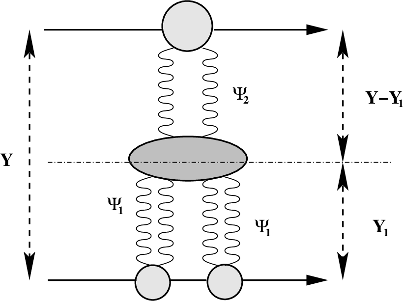
As an example of applications of the methods developed in the paper, we present calculations of the diffractive dissociation process in the RFT-0 with only triple Pomeron vertex. The algorithm of the calculations is defined as follows. We have the quantum solution of the theory
| (81) |
defined at all range of rapidity at some values of the sources and . Let’s now consider this solution at the rapidity interval . With the help of the we define another function
| (82) |
on the rapidity interval with the following initial condition:
| (83) |
The illustration of this construction see in the Fig.17.
The only numbers that we need to calculate now are the coefficients . But their calculation is trivial, they simply
| (84) |
where the weight function is the same as in the Eq.19. The coefficients fully determine requested function, which represents the differential cross section of the single diffraction process at given and fixed rapidity interval
Integrating this function over rapidity interval we obtain as the answer the sum of the total diffractive dissociation cross sections on this rapidity interval and elastic cross section
| (85) |
So, the value of the single difractive cross section integrated over rapidity interval is the following
| (86) |
where is the total rapidity of the process, is the rapidity ”gap” of the process, is the value of the rapidity taken by produced diffractive state and elastic cross section of the process is defined as . In general we do not expect that the numbers given by RFT-0 theory will be correct. The only interesting value in the given model, therefore, is the ratio of the single diffractive cross section to the total cross section.
| (87) |
where . Considering this ratio we can not prove, of course, that the same value of the we will obtain in QCD as well, but, nevertheless, it is interesting to see what new about this ratio we obtain using full quantum solution for the amplitudes. Another interesting ratio, which we can calculate in the given framework, this is a ratio of differential single diffraction cross section to the total cros section:
| (88) |
In ratio the dependence on diffractive mass is present, and it allows to as to trace the energy dependence of the ratio of the diffractive state to the total cross section. Therefore, the following calculations are presented. We fix the value of diffractive state equal 1-4 units of scaled rapidity as a one variable and as a second variable in the 3D plot we consider the value of total rapidity , which we take equal 4-8 units. These plots we make for the two different symmetrical values of the external sources: 0.2 and 0.7. Obtained plots, see Fig.18 for the ratio and Fig.19 for the ratio , show the changes of the ration accordingly to the total rapidity changes.
 |
 |
| Fig. (18)-a | Fig. (18)-b |
 |
 |
| Fig. (18)-c | Fig. (18)-d |
 |
 |
| Fig. (19)-a | Fig. (19)-b |
 |
 |
| Fig. (19)-c | Fig. (19)-d |
5 Discussion of results
The are the following main results of the paper. First of all, we obtained the full quantum solutions for the models and compared it with the classical solutions, illustrating the relative contribution of the loops to the amplitude. In order to find an useful approximation to the full quantum solution we also considered an eikonalized amplitude which was built with the help of the full two point Green’s functions. All these amplitudes were calculated for different values of external vertexes that allows to trace the applicability of each approximation separately in different parameter’s regions. Another important result is a comparison of quantum solutions with and without quaternary Pomeron vertex that clarify the contribution of this vertex to the process amplitude .
Plots Fig.4-Fig.9 represents the result of the calculations in the RFT-0 approach with triple Pomeron vertex only. The quantum solution of the model is presented in the plot Fig.4, whereas the classical solution is presented in the plot Fig.5. The comparison between these two solutions could be found in the plots Fig.6-Fig.7. From the Fig.4 we see, that our full solution for small values of external sources does not reach unitarity really. Instead of ”black” disk the ”grey” one is achieved. This is may be easily explained if we will remember that our initial conditions have a eikonal form, whereas in the s-channel model, see [35] and references therein, the propagator form of initial conditions is always applied. In RFT-0 model the black disk limit, as it must be, achieved only at large values of the sources, that corresponds to the nuclei interaction in usual QCD, see [21, 22, 38]. Other interesting results are represented in the Fig.6-Fig.7. Indeed, the natural question, which in fact is very important in any practical calculations with BK equation involved, is a question about applicability of classical solutions of the model. Namely, at which values of external sources the difference between the classical and quantum solutions is acceptable from the point of view of the precision of the amplitude calculations. In real QCD this answer may be obtained only approximately, at least. In RFT-0 calculations the answer is clear, at large values of the external sources the classical solution is acceptable only at large values of the sources. In the symmetrical case of interactions with the small sources involved, the relative difference between the amplitudes is very large. The difference pretty fast decreases with the increasing of the value of the sources, but still the difference is not negligible even when , see Fig.6-Fig.7. Important to underline, that one from the main reasons that provides the applicability of the classical solution is a presence of the third classical solution arose at some rapidity ( see Section 2.2 an Eq. (29)) in the framework. The third solution provides the decrease of the classical amplitude at large values of the total rapidity and without this solution the precision of the model was even worse. The situation with the non-symmetrical case of interactions is better, see Fig.8-Fig.9. Due the initially broken symmetry of the interaction, the fan diagrams are initially dominant and provide the better precision of the classical solution in comparison to the symmetrical case of interactions.
Considering the second possible candidate on the role of ”good amplitude approximation”, eikonalized function Eq. (39), see Fig.12, we see that at small values of the external sources this amplitude is indeed better than the classical solution. In the region of large values of the sources both amplitude are equal more or less - the unitarization corrections are small for the large sources. We also could compare the effective Pomeron propagator with the asymptotic results obtained in the framework of s-channel model, see [35]. Looking in the Fig.11 and Fig.16, we see, that the value of the full propagator, which considered as an amplitude in s-channel model, is close to one, especially for the second considered model with quaternary vertex included, which has direct relations with s-channel model, see again [35]. But, in general, for an arbitrary value of a source there is no propagator’s unitarization and the way to achieve the unitarization in this case is the eikonalization of the propagator only.
Interesting problem, which also could be investigated in the framework of RFT-0, is a problem of the influence of the value of the triple Pomeron vertex on the behavior of the amplitude. Changing value of the parameter from the till we change the value of the triple vertex from till . The resulting amplitude is depicted in the Fig.10. From this plot we see, that already at relatively small values of rapidity this amplitude is decreasing till zero. This fast of the decreasing of the amplitude at large values of denote a main difference between the models of RFT-0 with and without quaternary vertex. In RFT-0 without the quaternary vertex the amplitude, as it mentioned above, approaches zero whereas in RFT-0 with the quaternary vertex the amplitude approach constant with any value of triple vertex and correctly adjusted value of quaternary vertex, see Eq. (44), Eq. (74) and Eq. (76). Of course, when the value of the triple vertex is small, two models do not so differ, see Fig.15. This difference in the behavior of the amplitudes in two models may be also analyzed in the terms of s-channel model, see [35] for the details and explanations.
As a possible example of the application of the model we calculated the values of the ratios of the single diffractive and differential single diffractive cross sections to the total cross section in the given framework, see Eq.87 and Eq.88. The results of these calculations are present in the Fig.18 - Fig.19. The plot Fig.18 represents the ratio of single diffractive cross section (integrated over rapidity of the diffractive state) to the value of the total cross section. In two cases when the sources are equal 0.2 and 0.7, we obtain, that for the fixed value of the diffractive state this ratio almost does not change with energy. More precisely, in both cases there is a tiny change in the ratio behavior at small rapidities 4-5, and constant behavior at large rapidiies 6-8. Tracing the relative contribution of the diffractive state at fixed rapidity in both cases we see, that the contribution of the large mass diffractive state, , approximately two times large than the contribution from small , ”elastic”, diffractive state , as it must be in reality. We see, that the simple RFT-0 model correctly reproduce main futures of the real QCD. It is also interesting to note, that the relative contribution of the large mass diffractive state is larger for the case of small external sources, there is for source against for source . Concerning the calculations of the second ratio, , see Fig.19, we obtain that these two cases are different. At small source, , the maximum of the ratio is at small diffractive state, which has almost constant behavior with total rapidity. At large vale of source, , the situation is opposite, the maximim contribution comes from the large mass diffractive state. The contribution of the small diffractive state at is zero in Fig.19 at large values of Y, that means constant value of single diffraction cross section at small values of and large values of . In general, considering Fig.18 - Fig.19, we can conclude, that the description of the diffractive states in RFT in the case when we include in calculations all possible re-scattering corrections is different from the ”naive” diffraction models, where only part of corrections is included. Therefore, there is a hope, that using the same receipts of calculations in the QCD RFT, we will be able correctly describe diffraction data and their energy dependence.
6 Conclusion
In this paper we performed calculations of the different amplitudes in the framework of the RFT-0 model. Comparing different approximation we analyze the applicability of the different approximation schemes and their dependence on the parameters of the model. The main conclusion of the calculations is that we could trust to the classical approximation for the amplitude only when the value of the triple Pomeron vertex is small. In this region the difference between models with and without quaternary vertexes is negligible. Nevertheless, the important condition for this approximation in the case of interacting of symmetrical particles is an including of the third classical solution in the set of classical solutions, which arises at some critical value of rapidity. Without this solution the classical approximation is not good, even at not small values of the external sources. For the case of the small values of these vertexes the eikonalized Green’s function amplitude is more precise solution then the classical one. Unfortunately, in real QCD this amplitude also could not be calculated precisely and therefore we could not trust to the classical solutions at all when the values of the external sources is not large enough. Does the proton is ”large enough” in the case of real QCD is an open question, which could not be answered, unfortunately, in the given framework.
When the value of the triple vertex is growing, the picture is changing drastically. In this case we could not trust anymore to the classical solutions of the models. Also, there is a large difference in the behavior of the amplitude in models with and without quaternary vertex, it’s presence changes the asymptotic behavior of the amplitude. In real QCD it could means, that the different evolution equations must be applied in the different regions of the impact parameter space with the different values of the coupling constant. If we assume, that the influence of the non-perturbative effects is in the change of the value of the coupling constant only, then we must separate the contribution of the perturbative spots in impact parameter space, which evolution is described by the BK equation, from the non-perturbative regions where different evolution equations must be applied. In this case the overall amplitude is a sum of the amplitudes described by the different evolution equations in different regions, with the BK equation applicable in the regions of high partons density only. This picture will lead to the factorization of the non-perturbative effects from the perturbative ones, first of all, and also it could explain the possible applicability of the BK equation in case of proton-proton collisions. Namely, at high enough energies the overall contribution of ”black” spots may be larger then the contribution of the ”white” and ”grey” ones and we could describe even inclusive data by the BK equation formalism. The large but constant non-perturbative contributions into the amplitude in this case may be accounted by the adjusting of the values of the external sources in interaction of interests.
Concluding we underline, that RFT-0 model is a very interesting and important ground for an initial implementation of the different ideas which further could be applied in real QCD calculations as well.
Acknowledgments
I am grateful to Leszek Motyka for his participation in the development of the main themes of the paper and to M.Braun for his support and interest to the paper during period of it’s writing.
References
- [1] L. N. Lipatov, Sov. J. Nucl. Phys. 23 (1976) 338 [Yad. Fiz. 23 (1976) 642]; E. A. Kuraev, L. N. Lipatov and V. S. Fadin, Sov. Phys. JETP 45 (1977) 199 [Zh. Eksp. Teor. Fiz. 72 (1977) 377]; I. I. Balitsky and L. N. Lipatov, Sov. J. Nucl. Phys. 28 (1978) 822 [Yad. Fiz. 28 (1978) 1597].
- [2] L. N. Lipatov, Phys. Rept. 286 (1997) 131.
- [3] V. S. Fadin and L. N. Lipatov, Phys. Lett. B 429 (1998) 127; M. Ciafaloni and G. Camici, Phys. Lett. B 430 (1998) 349; V. S. Fadin and R. Fiore, Phys. Lett. B 610 (2005) 61 [Erratum-ibid. B 621 (2005) 61]; V. S. Fadin and R. Fiore, Phys. Rev. D 72 (2005) 014018.
- [4] J. Bartels, Z. Phys. C 60 (1993) 471.
- [5] J. Bartels and M. Wüsthoff, Z. Phys. C 66 (1995) 157.
- [6] J. Bartels and C. Ewerz, JHEP 9909 (1999) 026.
- [7] C. Ewerz, Phys. Lett. B 512 (2001) 239.
- [8] C. Ewerz and V. Schatz, Nucl. Phys. A 736 (2004) 371.
- [9] T. Bittig and C. Ewerz, Nucl. Phys. A 755 (2005) 616.
- [10] J. Jalilian-Marian, A. Kovner and H. Weigert, Phys. Rev. D 59 (1999) 014015; J. Jalilian-Marian, A. Kovner, A. Leonidov and H. Weigert, Phys. Rev. D 59 (1999) 014014; E. Iancu, A. Leonidov and L. D. McLerran, Nucl. Phys. A 692 (2001) 583; E. Iancu, A. Leonidov and L. D. McLerran, Phys. Lett. B 510 (2001) 133; E. Iancu and L. D. McLerran, Phys. Lett. B 510 (2001) 145; E. Ferreiro, E. Iancu, A. Leonidov and L. McLerran, Nucl. Phys. A 703 (2002) 489.
- [11] I. Balitsky, Nucl. Phys. B 463 (1996) 99; Y. V. Kovchegov, Phys. Rev. D 60 (1999) 034008; Y. V. Kovchegov, Phys. Rev. D 61 (2000) 074018.
- [12] A. H. Mueller, Nucl. Phys. B 415 (1994) 373.
- [13] E. Levin and K. Tuchin, Nucl. Phys. B 573 (2000) 833; M. Braun, Eur. Phys. J. C 16 (2000) 337; H. Weigert, Nucl. Phys. A 703 (2002) 823; N. Armesto and M. A. Braun, Eur. Phys. J. C 20 (2001) 517; K. Golec-Biernat, L. Motyka and A. M. Staśto, Phys. Rev. D 65 (2002) 074037; G. Chachamis, M. Lublinsky and A. Sabio Vera, Nucl. Phys. A 748 (2005) 649.
- [14] K. Golec-Biernat and A. M. Staśto, Nucl. Phys. B 668 (2003) 345.
- [15] K. Rummukainen and H. Weigert, Nucl. Phys. A 739 (2004) 183.
- [16] E. Levin and K. Tuchin, Nucl. Phys. A 691 (2001) 779; J. Kwieciński and A. M. Staśto, Phys. Rev. D 66 (2002) 014013; E. Iancu, K. Itakura and L. McLerran, Nucl. Phys. A 708 (2002) 327.
- [17] A. H. Mueller and D. N. Triantafyllopoulos, Nucl. Phys. B 640 (2002) 331; D. N. Triantafyllopoulos, Nucl. Phys. B 648 (2003) 293; L. Motyka, Phys. Lett. B, in print; arXiv:hep-ph/0509270.
- [18] E. Gotsman, E. Levin, M. Lublinsky and U. Maor, Eur. Phys. J. C 27 (2003) 411;
- [19] K. Kutak and J. Kwieciński, Eur. Phys. J. C 29 (2003) 521; K. Kutak and A. M. Staśto, Eur. Phys. J. C 41 (2005) 343.
- [20] E. Iancu, K. Itakura and S. Munier, Phys. Lett. B 590 (2004) 199.
- [21] M. A. Braun, Phys. Lett. B 483 (2000) 115.
- [22] M. A. Braun, Eur. Phys. J. C 33 (2004) 113.
- [23] M. A. Braun, Phys. Lett. B 632 (2006) 297.
- [24] L. N. Lipatov, Nucl. Phys. B 452 (1995) 369.
- [25] A. Kovner and M. Lublinsky, Phys. Rev. Lett. 94 (2005) 181603; J. P. Blaizot, E. Iancu, K. Itakura and D. N. Triantafyllopoulos, Phys. Lett. B 615 (2005) 221; Y. Hatta, E. Iancu, L. McLerran, A. Staśto and D. N. Triantafyllopoulos, Nucl. Phys. A 764 (2006) 423; C. Marquet, A. H. Mueller, A. I. Shoshi and S. M. H. Wong, Nucl. Phys. A 762 (2005) 252.
- [26] I. Balitsky, Phys. Rev. D 75 (2007) 014001; I. Balitsky and G. A. Chirilli, Phys. Rev. D 77 (2008) 014019; Y. V. Kovchegov and H. Weigert, Nucl. Phys. A 784 (2007) 188; J. L. Albacete and Y. V. Kovchegov, Phys. Rev. D 75 (2007) 125021.
- [27] J. Bartels, M. G. Ryskin and G. P. Vacca, Eur. Phys. J. C 27, 101 (2003); M. A. Braun, Eur. Phys. J. C 63, 287 (2009).
- [28] D. Amati, L. Caneschi and R. Jengo, Nucl. Phys. B 101 (1975) 397.
- [29] R. Jengo, Nucl. Phys. B 108 (1976) 447; D. Amati, M. Le Bellac, G. Marchesini and M. Ciafaloni, Nucl. Phys. B 112 (1976) 107; M. Ciafaloni, M. Le Bellac and G. C. Rossi, Nucl. Phys. B 130 (1977) 388.
- [30] M. Ciafaloni, Nucl. Phys. B 146 (1978) 427.
- [31] A. H. Mueller, Nucl. Phys. B 437 (1995) 107; P. Rembiesa and A. M. Stasto, Nucl. Phys. B 725, 251 (2005); A. I. Shoshi and B. W. Xiao, Phys. Rev. D 73 (2006) 094014; M. Kozlov and E. Levin, Nucl. Phys. A 779, 142 (2006); A. I. Shoshi and B. W. Xiao, Phys. Rev. D 73, 094014 (2006); M. A. Braun and G. P. Vacca, Eur. Phys. J. C 50, 857 (2007); J. P. Blaizot, E. Iancu and D. N. Triantafyllopoulos, Nucl. Phys. A 784, 227 (2007); N. Armesto, S. Bondarenko, J. G. Milhano and P. Quiroga, JHEP 0805, 103 (2008).
- [32] S. Bondarenko and L. Motyka, Phys. Rev. D 75, 114015 (2007).
- [33] S. Bondarenko and M. A. Braun, Nucl. Phys. A 799, 151 (2008).
- [34] M. A. Braun, Nucl. Phys. A 806 (2008) 230.
- [35] S. Bondarenko, L. Motyka, A.H. Mueller, A.I. Shoshi and B.-W.Xiao, Eur. Phys. J. C 50, 593 (2007).
- [36] G. P. Korchemsky, Nucl. Phys. B 550, 397 (1999).
- [37] S. Bondarenko, Nucl. Phys. A 792, 264 (2007)
- [38] S. Bondarenko, E. Gotsman, E. Levin and U. Maor, Nucl. Phys. A 683, 649 (2001).