Optimal Distributed Beamforming for MISO Interference Channels
Abstract
We consider the problem of quantifying the Pareto optimal boundary in the achievable rate region over multiple-input single-output (MISO) interference channels, where the problem boils down to solving a sequence of convex feasibility problems after certain transformations. The feasibility problem is solved by two new distributed optimal beamforming algorithms, where the first one is to parallelize the computation based on the method of alternating projections, and the second one is to localize the computation based on the method of cyclic projections. Convergence proofs are established for both algorithms.
Index Terms:
MISO-Interference Channel, Distributed Beamforming, Achievable Rate Region, Pareto OptimalI Introduction
Traditional wireless mobile systems are designed with the cellular architecture, in which neighboring base stations (BSs) in different cells try to manage communications for their intended mobile stations (MSs) over non-overlapping channels. The associated inter-cell interferences, from non-neighboring cells, are treated as additive background noises. To improve the performance of traditional systems, most beyond-3G wireless technologies relax the frequency reuse constraint such that the whole frequency band becomes available for all cells. As such, joint signal processing across neighboring BSs is needed to cope with the strong inter-cell interferences in the future cellular systems.
In this paper, we study a particular type of multi-BS cooperation for downlink transmissions, where we assume a scenario with each BS equipped with multiple antennas and each MS equipped with a single antenna. Besides, only one MS is assumed to be active in each cell at any given time (over a particular frequency band). Our problem setup can be modeled as a multiple-input single-output (MISO) Gaussian interference channel (IC), termed as MISO-IC.
From an information-theoretic viewpoint, the best achievable rate region to date for an IC was established by Han and Kobayashi in [1], termed as the Han-Kobayashi region, which utilizes rate splitting at transmitters, joint decoding at receivers, and time sharing among codebooks. The Han-Kobayashi region was simplified in [2] and proved to be within 1-bit of the capacity region of the Gaussian IC in [3]. However, in cellular systems, practical constraints often limit MSs to only implement single-user detection (SUD) schemes, i.e., treating the interference from all other unintended BSs as noise. Hence, in this work, we assume SUD at the MS receivers. With SUD, it has been shown that transmit beamforming is optimal for MISO IC in [4] and [5]. For the two-user case, Jorswieck et al. [6] proved that the Pareto-optimal beamforming vectors can be represented as linear combinations of the zero-forcing (ZF) and maximum-ratio transmission (MRT) beamformers. Previous studies [7] and [8] over MISO-IC beamforming usually assumed a central processing unit with global knowledge of all the downlink channels, which may not be feasible in practical systems. To make the result more implementable, our work focuses on multi-cell cooperative downlink beamforming, which involves distributed computations based on the local channel knowledge at each BS. Such decentralized multi-cell cooperative beamforming problems were previously studied in [9] based on the uplink-downlink duality to minimize the sum transmission power. Furthermore, a heuristic decentralized algorithm was developed in [4] for multi-cell cooperative downlink beamforming based on the iterative updates of certain interference-temperature constraints across different pairs of BSs.
It has been discussed in [4] that quantifying the Pareto optimal points in the achievable rate region over MISO IC may boil down to solving a sequence of convex feasibility problems after certain transformations, where the feasibility problems can be recast as second-order cone programming (SOCP) problems as shown in [10]. In this paper, we propose two algorithms to solve the resulting feasibility problem parallelly or distributively. In the first parallized beamforming algorithm based on alternating projections, we assume a computation-power limited centralized processing unit such that part of the computation duties need to be parallely conducted in each individual BS. In the second beamforming algorithm, localized sequential optimizations across the BSs are performed iteratively, where the need for a central processing unit is eliminated. Convergence in norm for both algorithms is established. Besides, a set of feasibility decision rules is established to implement our algorithms for practical engineering applications.
The rest of the paper is organized as follows. Section II presents the MISO-IC model for multi-cell downlink beamforming, defines the Pareto optimality, and reviews the rate profile approach, which transforms the whole problem into solving a sequence of SOCP feasibility problems. Section III proposes the parallelized algorithm to parallelly solve the SOCP feasibility problem based on the method of alternating projections. Section IV presents the distributed beamforming algorithm to solve the SOCP feasibility problem based on the method of cyclic projections. Numerical examples are provided in Section V with conclusions in Section VI.
Notations: Bold face letters, e.g., and , denote vectors and matrices, respectively. and denote the identity matrix and the all-zero matrix, respectively, with appropriate dimensions. defines a block diagonal matrix in which the diagonal elements are . and respectively denote the transpose and the Hermitian of a matrix or a vector. and denote the space of real matrices and the space of complex matrices respectively. denotes the Euclidean norm of a complex vector . All the functions are with base 2 by default. and denote the real part and imaginary part of a complex argument respectively. defines a vector that stacks into one column. By default, all the vectors are column vectors.
II System Model and Preliminaries
II-A Signal Model
We address downlink transmissions in a cellular network consisting of cells, each having a multi-antenna BS to transmit an independent message to one active single-antenna MS. With the assumption that the same band is shared among all BSs for downlink transmissions, the system could be modeled as a -user MISO-IC. Specifically, we assume that each BS is equipped with transmitting antennas, . With the assumption of single-user detection at each receiver, it has been shown in [4] and [5] that beamforming is optimal to maximize the rate region. Hence, the discrete-time baseband received signal of the active MS in the th cell is given by
| (1) |
where denotes the beamforming vector at the th BS; denotes the channel vector from the th BS to its intended MS, while denotes the cross-link channel from the th BS to the MS in the th cell, ; denotes the symbol transmitted by the th BS; and denotes the additive circular symmetric complex Gaussian (CSCG) noise at the th receiver. It is assumed that and ’s are independent.
We assume that the th receiver only knows channel , and decodes its own messages by treating interferences from all other BSs as noise. With SUD, the achievable rate for the th MS is thus given as
| (2) |
where the maximum transmission power is limited as
| (3) |
where is the power constraint at the th BS.
II-B Pareto Optimality
We define the achievable rate region for the MISO-IC to be the collection of rate-tuples for all MSs that can be simultaneously achievable under a certain set of transmit-power constraints:
The upper-right boundary of this region is called the Pareto boundary, since it consists of rate-tuples at which it is impossible to increase some user’s rate without simultaneously decreasing the rate of at least one other users. To be more precise, the Pareto optimality of rate-tuple is defined as follows [6].
Definition 1
A rate-tuple is Pareto optimal if there is no other rate-tuple with and , with the inequality being component-wise.
In this paper, we are interested in searching the beamforming vectors for all BSs that lead to Parato optimal rate-tuples.
II-C Rate Profile Approach
The rate profile approach [11] is an effective way to characterize the Pareto boundary of MISO-IC [4], where the key is that any rate tuple on the Pareto boundary can be obtained by solving the following optimization problem given a specified rate-profile vector, :
| (7) | |||||
where satisfies that , and . Denote the optimal objective value of Problem (7) as . As shown in [4], corresponds to a particular Pareto optimal rate tuple. Hence, by exhausting all possible values for , solving Problem (7) yields the whole Pareto boundary.
II-D SOCP Feasibility Problem
Directly solving Problem (7) is usually difficult due to its non-convexity. However given the fact that the objective function is a single variable, we could adopt the bisection search algorithm to efficiently find as shown in [4]. Specifically, we could solve a sequence of the following feasibility problems each for a given :
| (8) | |||||
Therefore if the above problem is feasible for , it follows that ; otherwise, . Hence, a bisection search over can be done. However, Problem (8) is still non-convex.
As shown in [10], we can adjust the phase of in (8) to make real and non-negative without affecting the value of . Hence, by denoting , Problem (8) can be recast as
| (9) |
We further define , , with , and . For convenience, we add a term to both sides of the first constraint in Problem (9) as
| (10) |
where . Finally, with our newly defined variables and coefficients, we recast Problem (9) as
| (11) |
where vector is of the same dimension as with all zero elements except for the last one being 1, such that the last element of is guaranteed to be 0.
Consequently, Problem (11) is a SOCP problem, which can be efficiently solved by numerical tools [12]. However, directly solving Problem (11) requires a centralized algorithm running at a control center, which may not be desired in certain engineering applications. Accordingly, there are usually two motivations for seeking distributed algorithms: one is to decompose the computations into multiple sub-programs such that the requirement for the central processing power is reduced; and the other is to localize computations such that no central control facility is required. In Section III and Section IV, we propose two algorithms based upon the above two motivations, respectively.
III Alternating Projections Based Distributed Beamforming
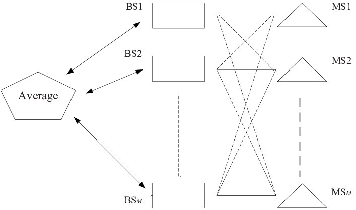
In this section, in order to reduce the requirement on processing power at the control center, we develop a downlink beamforming algorithm, termed as alternating projections based distributed beamforming (APB), to solve Problem (11) parallelly in sub-problems. With our algorithm, the only processing power needed at the central unit is to calculate an average value over all the localized solutions from the BSs. The algorithm is iterative, where parallel optimizations across BSs are performed at each round. The convergence issue of APB is also studied in this section.
III-A APB Algorithm
At the initialization stage, the computation-limited centralized unit is assigned with the values for , , and . Then the central unit broadcasts the information to all BSs with an arbitrary initial point . It is assumed that the th BS has the perfect knowledge of the channels from all BSs to the th MS, i.e., all ’s. Furthermore, all BSs operate according to the same protocol described as follows. At the th round, we denote the solution vector that the central unit broadcasts as . Then at the th BS, the corresponding problem is expressed as
| (12) | |||||
where , with denoting the optimal solution for Problem (12) of the ()th round at the th BS. A rough description of the algorithm is depicted in Fig. 1.
Remark 1
Note that if Problem (12) is infeasible at the th BS (), we can directly claim that the associated Problem (11) is infeasible and quit APB. As such, from now on we only focus on the cases where Problem (12) is always feasible at each individual BS, and run APB to check when the overall problem in (11) is feasible and when it is not. With a feasible Problem (12), we need the optimal solution to satisfy all the transmitter power constraints and the th receiver’s SNR demand. The reason why we keep all power constraints at each individual BS is for that fast convergence, which can be observed from simulations. Since all the values are typically predetermined in cellular systems, no extra system overhead is needed. In the second-order cone constraint of Problem (12), directly using the term implies that and .
III-B Convergence Analysis
Since APB is iterative, the convergence is an important issue to address. The convergence of APB is formally stated as follows.
Proposition 1
As increases, the optimal solution for Problem (12) converges in norm to the limit when Problem (11) is either feasible or infeasible. Furthermore, the averaged solution also converges in norm to satisfying that . In particular, if Problem (11) is feasible, all ’s coincide in the same point that lies in the feasible set of Problem (11) with . If Problem (11) is infeasible, ’s do not coincide in the same solution.
Proof: 1) For the case of Problem (11) being feasible, we have the following proof.
We first introduce the concept of finding the closest point to some given point in a closed convex set and alternating projections.
In mathematics, a Hilbert space is defined with the inner product and the induced norm . If is a nonempty closed convex set in , Riesz [13] states that each has a unique best approximation (or nearest point) in . That is, . The mapping is called the projection onto , i.e., finding the closest point to in a closed nonempty convex set. In this paper, we use the general Euclidean inner product definitions in the complex space and in the real space.
Definition 2
Suppose and are two closed nonempty convex sets in with corresponding projections and . Let and fix a starting point . Then the sequence of alternating projections is generated by
Let denote the feasible set of Problem (12) at the th BS, , and ; note that is exactly the feasible set of Problem (11). Thus solving Problem (12) at the th BS can be viewed as finding the closest point to in a non-empty closed convex set , i.e., the projection of onto . Next we transform the variable defined over the complex Hilbert space to a double-dimensioned real Hilbert space such that we can use some existed results in alternating projections. We transform to by letting , where . Similarly, we map the complex set to a double-dimensioned real set , and map to a double-dimensioned real vector . We rewrite Problem (12) as
| (13) | |||||
where
From the constraints of Problem (13), we observe that the feasible set is the intersection of a collection of second-order cones, some subspaces, and some norm balls, which is nonempty closed and bounded. Next we show how to transform our algorithm into a problem of alternating projections. Let’s define two product sets:
and
Meanwhile£¬ we define two new variables as
| (14) |
Obviously, . By the results of Pierra in [14], we have the following two lemmas:
Lemma 1
Solving Problems (12) for in parallel at the th round is equivalent to projecting vector onto the closed convex set and obtaining .
Lemma 2
Computing is equivalent to projecting onto and getting .
Therefore, APB can be interpreted as alternating projections between and . Note that the idea of Alternating Projections was first proposed by von Neumann in [15], where only subspaces are assumed as the projection sets. Then many researchers extended this technique to more general scenarios [16], [17]. For alternating projections between two non-empty closed convex sets and , Cheney [16] proved that convergence in norm is always assured when either (a) one set is compact, or (b) one set is of finite dimension. Since set is bounded and our underlying Hilbert space is of finite dimension, both conditions (a) and (b) are satisfied. Therefore, APB always leads to strong convergence, i.e., convergence in norm, due to the facts that the numbers of cells and antennas are always finite. As shown in [17], all ’s will coincide into the same point that lies in .
2) For the case of Problem (11) being infeasible, we have the following proof.
With , the convergence of APB is still equivalent to the convergence of alternating projections between and , where Cheney’s results in [16] are applicable in this case. Thus, the convergence in norm is still valid for infeasible cases. Besides, it is easy to verify that . However, ’s do not coincide into the same point.
We now complete the proof for Proposition 1.
III-C Practical Feasibility Decision Rules
With convergence in norm for APB established, we now need to establish some practical feasibility check rules to correctly terminate APB when it converges.
From Lemma 1 and Lemma 2, we know that the feasibility of Problem (11) is totally determined by whether and intersect or not. By Proposition 1, if Problem (11) is feasible, all convergent solutions coincide at a common point which belongs to . In this case, all optimal values of Problems (12) converge to 0. On the other hand, if any of the optimal values of Problems (12) do not converge to 0, Problem (11) is infeasible. Based on the above discussions, we develop the following APB terminating procedures:
Step 1: We set two threshold parameters and . The selection of and affects the effectiveness of the algorithm.
Step 2: Initialization: Let be the optimal value of Problem (12) at the th cell in the current computation round, be the optimal value Problem (12) at the th cell in the previous computation round, and , be the flags for the BSs. At the beginning, we set and all zeros.
Step 3: Repeat: For , the th BS solves Problem (12) and compares against . If , we refresh and proceed to Step 4; if , we compare with : If , we claim that Problem (11) is infeasible and stop; otherwise, we mark this cell as and proceed to Step 4.
Step 4: If for all , we claim that the Problem (11) is feasible, then stop. Otherwise, return to Step 3.
Remark 2
Note that here we applied several approximations in making the decisions. First, we claim that Problem (12) at the th BS converges when . Thus, is considered as the limit of th BS’s optimal solution. Second, we set as the threshold dividing zero and non-zero values: If , we consider the limit non-zero, and vice versa. In simulations, we usually set both and small with . For example, and are chosen for the simulation results in Section V.
IV Cyclic Projections Based Distributed Beamforming
In this section, to localize computations such that no central control unit is required, we propose a decentralized algorithm that practically implements the multi-cell cooperative downlink beamforming. It is still assumed that the th BS in the cellular network has the perfect knowledge of the channels from all BSs to the th MS. Similar to APB, we decompose Problem (11) to sub-problems and compute them at BSs individually. In particular, the problems are solved sequentially at each round, and the algorithm proceeds iteratively, which is termed as Cyclic Projections Based Distributed Beamforming (CPB).
IV-A CPB Algorithm
A certain cyclic update order among the BSs needs to be determined at the initialization stage, where the 1st BS sends its solution to the 2nd, , the ()th BS sends its solution to the th BS, and the th BS sends its solution to the 1st, in a cyclic fashion. At the beginning, the BSs should obtain the values for , , and . The algorithm starts from the 1st BS, after choosing an arbitrary initial point , it solves the following problem
| (15) | |||||
where the optimal solution for the above problem is labelled as and sent to the 2nd BS. Then the other BSs begin to solve their own problems sequentially according to the predefined order. In particular, at the th round the th BS () solves the following problem
| (16) | |||||
where is the solution sent over by the preceding BS, and is used to denote the newly solved optimal solution. For simplicity, we refer the problem in (16) as a cyclic subproblem. Such a scheme is illustrated in Fig. 2.

IV-B Convergence Analysis
We first introduce the concept of cyclic projections.
Definition 3
Suppose are closed convex sets in the Hilbert space with , and let be the projection for , . The operation of cyclic projections is an iterative process that can be described as follows. Start with any point , and define the sequence () by
| (17) |
where is the projection operator to .
In the literature, Bregman [18] showed that the above sequence generated by cyclic projections always converges weakly to some point provided that , and Gubin [19] et al. provided a systematic study over general cyclic projections including the case of . Based on these results, we have the following proposition.
Proposition 2
Proof: It is obvious that the optimal solutions for cyclic subproblems in (16) form a sequence of cyclic projections. Since weak convergence is always guaranteed [18], by the equivalence of weak convergence and convergence in norm in a finite dimensional space [20], we obtain Proposition 2.
Remark 4
Note that the convergence proof of CPB is more general than that of APB since alternating projections is actually a special case of cyclic projections where the number of projection sets is two.
IV-C Practical Feasibility Decision Rules
For CPB, the algorithm termination rules are similar to that of APB, which is skipped here.
V Simulation Results
The performance of APB is first simulated. In the simulations, we set and . We set the power constraints as 15, 18, and 21, respectively, for the three BSs. In Fig. 3, we demonstrates the convergence behavior as described in Proposition 1. The three curves correspond to the required SNR ’s as 5, 10, and 20, respectively. We observe that their asymptotic behaviors are similar. In Fig. 4, with a feasible choice of , , we draw how the achieved SNR values approach the target values over iterations. If Problem (11) is infeasible, for example, when setting target SNR as , the SNR evolution curves are given in Fig. 5, where we see that none of the target SNRs are satisfied.
For the performance of CPB, the simulation setup is exactly the same as that for APB. In Fig. 6, with a feasible choice of , , we see how the achieved SNR values approach the target values with less iterations needed compared with Fig. 4.
We observe from multiple simulations that the convergence speed of CPB is much faster than APB.
VI Concluding Remarks
In this paper, based on alternating projections and cyclic projections, we have developed two optimal distributed beamforming schemes to cooperatively solve the SOCP feasibility problem that is the key for quantifying the Pareto optimal points in the achievable rate region of MISO interference channels. The convergence in norm for both algorithms was established, which was further verified by numerical simulations.


References
- [1] T. S. Han and K. Kobayashi, “A new achievable rate region for the interference channel,” IEEE Trans. Inf. Theory, vol. 27, no. 1, pp. 49-60, Jan. 1981.
- [2] H. F. Chong, M. Motani, H. K. Garg, and H. El. Gamal, “On the Han-Kobayashi region for the interference channel,” IEEE Trans. Inf. Theory, vol. 54, no. 7, pp. 3188-3195, Jul. 2008.
- [3] R. H. Etkin, D. N. C. Tse, and H. Wang, “Gaussian interference channel capacity to within one bit,” IEEE Trans. Inf. Theory, vol. 54, no. 12, pp. 5534-5562, Dec. 2008.
- [4] R. Zhang and S. Cui, “Cooperative interference management in multi-cell downlink beamforming,” IEEE Trans. Sig. Process., vol. 58, no. 10, pp. 5450-5458, Oct. 2010.
- [5] X. Shang, B. Chen, H. V. Poor, “Multi-user MISO interference channels with single-user detection: optimality of beamforming and the achievable rate region,” submitted to IEEE Trans. Inf. Theory, May, 2009.
- [6] E. A. Jorswieck, E. G. Larsson, and D. Danev, “Complete characterization of the Pareto boundary for the MISO interference channel,” IEEE Trans. Sig. Process., vol. 56, no. 10, pp. 5292-5296, Oct. 2008.
- [7] S. Shamai (Shitz) and B. M. Zaidel, “Enhancing the cellular downlink capacity via co-processing at the transmitting end,” in Proc. IEEE Veh. Technol. Conf. (VTC), vol. 3, pp. 1745-1749, May 2001.
- [8] O. Somekh, B. Zaidel, and S. Shamai (Shitz), “Sum rate characterization of joint multiple cell-site processing,” IEEE Trans. Inf. Theory, vol. 53, no. 12, pp. 4473-4497, Dec. 2007.
- [9] H. Dahrouj and W. Yu, “Coordinated beamforming for the multi-cell multi–antenna wireless system,” in Proc. Conf. Inf. Sciences and Systems (CISS), Mar. 2008.
- [10] M. Bengtsson and B. Ottersten, “Optimal downlink beamforming using semidefinite optimization,” in Proc. Annual Allerton Conf. Commun., Control and Comput., pp. 987-996, Monticello, Illinois, Sept. 1999.
- [11] M. Mohseni, R. Zhang, and J. M. Cioffi, “Optimized transmission for fading multiple-access and broadcast channels with multiple antennas,” IEEE Journal of Sel. Areas Commun., vol. 24, no. 8, pp. 1627-1639, Aug. 2006.
- [12] S. Boyd and L. Vandenberghe, Convex Optimization, Cambridge University Press, 2004.
- [13] F. Riesz, “Zur Theorie des Hilbertschen Raumes,” Acta Sci. Math. Szeged, vol. 7, pp. 34-38, 1934.
- [14] G. Pierra, “Decomposition through formalization in a product space,” Math. Programming, 28, pp. 96-115, 1984.
- [15] J. von Neumann, Functional Operators, Vol. II, Princeton University Press, 1950. (Reprint of mimeographed lecture notes first distributed in 1933.)
- [16] W. Cheney and A. A. Goldstein. “Proximity maps for convex sets,” in Proc. Am. Math. Soc., vol. 10, no. 3, pp. 448-450, 1959.
- [17] H. H. Bauschke and J. M. Borwein, “On the convergence of von Neumann’s alternating projection algorithm for two sets,” Set-Valued Analysis, vol. 1, no. 2, pp. 185-212, 1993.
- [18] L. M. Bregman, “The method of successive projection for finding a common point of convex sets,” Soviet Math. Dokl., vol. 6, pp. 688-692, 1965.
- [19] L. G. Gubin, B. T. Polyak, and E. V. Raik, “The method of projections for finding the common point of convex sets,” U.S.S.R. Comput. Math. and Math. Phys., pp. 1-24, 1967.
- [20] F. Deutsch and H. Hundal, “The rate of convergence for the cyclic projections algorithm I: Angles between convex sets,” Journal of Approximation Theory, 142(1), pp. 36-55, 2006.