跳到论文正文
W Papers独立论文阅读器 arXiv:1011.3760 论文正文 计算阅读时间 · 0%
引用这篇论文根据当前论文元数据生成,正式投稿前建议核对。


License: arXiv.org perpetual non-exclusive license
arXiv:1011.3760v3 [hep-th] 31 Jan 2011

Entanglement Entropy of Two Black Holes and
Entanglement Entropic Force

Preprint: OU-HET 683/2010
Noburo Shiba Email: shiba@het.phys.sci.osaka-u.ac.jp Affiliation: Department of Physics, Graduate School of Science, Osaka University, Toyonaka, Osaka 560-0043, Japan
August 24, 2026
Abstract

We study the entanglement entropy, SCS_{C}, of the massless free scalar field on the outside region CC of two black holes AA and BB whose radii are R1R_{1} and R2R_{2} and how it depends on the distance, r(≫R1,R2)r(\gg R_{1},R_{2}) , between two black holes. If we can consider the entanglement entropy as thermodynamic entropy, we can see the entropic force acting on the two black holes from the rr dependence of SCS_{C}. We develop the computational method based on that of Bombelli et al to obtain the rr dependence of SCS_{C} of scalar fields whose Lagrangian is quadratic with respect to the scalar fields. First we study SCS_{C} in d+1d+1 dimensional Minkowski spacetime. In this case the state of the massless free scalar field is the Minkowski vacuum state and we replace two black holes by two imaginary spheres, and we take the trace over the degrees of freedom residing in the imaginary spheres. We obtain the leading term of SCS_{C} with respect to 1/r1/r. The result is SC=SA+SB+1r2​d−2​G​(R1,R2)S_{C}=S_{A}+S_{B}+\tfrac{1}{r^{2d-2}}G(R_{1},R_{2}), where SAS_{A} and SBS_{B} are the entanglement entropy on the inside region of AA and BB, and G⁡(R1,R2)≤0G(R_{1},R_{2})\leq 0. We do not calculate G⁡(R1,R2)G(R_{1},R_{2}) in detail, but we show how to calculate it. In the black hole case we use the method used in the Minkowski spacetime case with some modifications. We show that SCS_{C} can be expected to be the same form as that in the Minkowski spacetime case. But in the black hole case, SAS_{A} and SBS_{B} depend on rr, so we do not fully obtain the rr dependence of SCS_{C}. Finally we assume that the entanglement entropy can be regarded as thermodynamic entropy, and consider the entropic force acting on two black holes. We argue how to separate the entanglement entropic force from other force and how to cancel SAS_{A} and SBS_{B} whose rr dependence are not obtained. Then we obtain the physical prediction which can be tested experimentally in principle.

pacs
03.65.Ud, 04.70.Dy, 11.90.+t

I Introduction

Entanglement entropy in quantum field theory (QFT) was originally studied to explain the black hole entropy [1, 2]. Entanglement entropy is generally defined as the von Neumann entropy SA=−T​r​ρA​ln⁡ρAS_{A}=-Tr\rho_{A}\ln\rho_{A} corresponding to the reduced density matrix ρA\rho_{A} of a subsystem AA. When we consider quantum field theory in d+1d+1 dimensional spacetime ℝ×N\mathbb{R}\times N, where ℝ\mathbb{R} and NN denote the time direction and the dd dimensional space-like manifold respectively, we define the subsystem by a dd dimensional domain A⊂NA\subset N at fixed time t=t0t=t_{0}. (So this is also called geometric entropy.) Entanglement entropy naturally arises when we consider the black hole because we cannot obtain the information in the black hole. In fact, in the vacuum state the leading term of the entanglement entropy of AA is proportional to the area of the boundary ∂A\partial A in many cases [1, 2]. This is similar to the black hole entropy, and extensive studies have been carried out [3, 4, 5, 6, 7, 8].

In this paper we study the entanglement entropy, SCS_{C}, of the massless free scalar field on the outside region CC of two black holes AA and BB whose radii are R1R_{1} and R2R_{2} and how it depends on the distance, r(≫R1,R2)r(\gg R_{1},R_{2}) , between two black holes. We consider the case that the state of the massless free scalar field is the vacuum state which depends how to choose the time coordinate. We choose the coordinate system which covers whole space time and does not have the coordinate singularity on the horizons. If we can consider the entanglement entropy as thermodynamic entropy, we can see the entropic force (we call this entanglement entropic force) acting on the two black holes from the rr dependence of SCS_{C}.

In Section II we obtain the general behavior of the entanglement entropy of two disjoint regions in translational invariant vacuum in general QFT. In Section III we review the computational method of entanglement entropy in free scalar fields [1]. There are some computational methods of entanglement entropy [9, 10, 11] . See [12, 13] for reviews. That of Bombelli et al [1] is most straightforward and powerful enough to obtain the rr dependence of SCS_{C} in free scalar field theory. In Section IV we study SCS_{C} in d+1d+1 dimensional Minkowski spacetime. In this case the state of the massless free scalar field is the Minkowski vacuum state and we replace two black holes by two imaginary spheres, and we take the trace over the degrees of freedom residing in the imaginary spheres. We develop the method of Bombelli et al and obtain the leading term of SCS_{C} with respect to 1/r1/r. The result in this section agrees with the general behavior in Section II. This method can be used for any scalar fields in curved space time whose Lagrangian is quadratic with respect to the scalar fields (i.e higher derivative terms can exist). In Section V we consider the black hole case. We use the method used in Section IV with some modifications. We show that SCS_{C} can be expected to be the same form as that in the Minkowski spacetime case. But in the black hole case SAS_{A} and SBS_{B} depend on rr, so we do not fully obtain the rr dependence of SCS_{C}. In Section VI we assume that the entanglement entropy can be regarded as thermodynamic entropy, and consider the entanglement entropic force. We argue how to separate the entanglement entropic force from other force and how to cancel SAS_{A} and SBS_{B} whose rr dependence are not obtained. Then we obtain the physical prediction which can be tested experimentally in principle, and discuss the possibility to measure the entanglement entropic force. In Appendix B we obtain a formula for a finite series as a by-product of our calculation.

II general behavior

We consider entanglement entropy of two disjoint regions (AA and BB) in translational invariant vacuum in general QFT in d+1d+1 dimensional spacetime (d≥2)(d\geq 2). We will show that SCS_{C} reaches its maximum value when r→∞r\rightarrow\infty.

There are several useful properties which entanglement entropy enjoys generally.(See e.g. [14].) We summarize some of them for later use.
1. If a composite system AB is in a pure state, then SA=SBS_{A}=S_{B}.
2. If ρA​B=ρA⊗ρB\rho_{AB}=\rho_{A}\otimes\rho_{B}, then SA​B=SA+SBS_{AB}=S_{A}+S_{B}.
3. For any subsystem AA and BB, the following inequalities hold:

SA​B≤SA+SB,\displaystyle S_{AB}\leq S_{A}+S_{B}, (1)
SA​B≥∣SA−SB∣.\displaystyle S_{AB}\geq\mid S_{A}-S_{B}\mid. (2)

The first is the subadditivity inequality, and the second is the triangle inequality.

Because of translational invariance, SAS_{A} and SBS_{B} are independent of their positions, so,∂SA∂r=0\tfrac{\partial S_{A}}{\partial r}=0 and ∂SB∂r=0\tfrac{\partial S_{B}}{\partial r}=0. And the total system is in a pure state, so we have SC=SA​BS_{C}=S_{AB}. Moreover, in the vacuum state, limr→∞ρA​B=ρA⊗ρB\lim_{r\rightarrow\infty}\rho_{AB}=\rho_{A}\otimes\rho_{B} because of the cluster decomposition principle [16]. So the property 2 suggests

limr→∞SC​(r)=SA+SB.\lim_{r\rightarrow\infty}S_{C}(r)=S_{A}+S_{B}. (3)

We apply (1) and (2)to this system, then we obtain

∣SA−SB∣≤SC​(r)≤SA+SB.\mid S_{A}-S_{B}\mid\leq S_{C}(r)\leq S_{A}+S_{B}. (4)

Eqs. (3) and (4) show that SCS_{C} (as a function of rr) reaches its maximum value when r→∞r\rightarrow\infty.

III how to compute entanglement entropy

In this section we review the computational method developed by Bombelli et al [1].

III.1 Entanglement entropy of a collection of coupled harmonic oscillators

We model the scalar field on ℝd\mathbb{R}^{d} as a collection of coupled oscillators on a lattice of space points, labeled by capital Latin indices, the displacement at each point giving the value of the scalar field there. In this case the Lagrangian can be given by

L=12​GM​N​q˙M​q˙N−12​VM​N​qM​qN,L=\dfrac{1}{2}G_{MN}\dot{q}^{M}\dot{q}^{N}-\dfrac{1}{2}V_{MN}q^{M}q^{N}, (5)

where qMq^{M} gives the displacement of the Mth oscillator and q˙M\dot{q}^{M} its generalized velocity. The symmetric matrix GM​NG_{MN} is positive definite, and therefore invertible, i.e, there exists the inverse matrix GM​NG^{MN} such that

GM​P​GP​N=δNM.G^{MP}G_{PN}=\delta^{M}_{~~N}. (6)

The matrix VM​NV_{MN} is also symmetric and positive definite. Next, consider the positive definite symmetric matrix WM​NW_{MN} defined by

WM​A​GA​B​WB​N=VM​N.W_{MA}G^{AB}W_{BN}=V_{MN}. (7)

The matrix WW is the square root of VV in the scalar product GG.

Now consider a region Ω\Omega in ℝd\mathbb{R}^{d}. The oscillators in this region will be specified by Greek letters, and those in the complement of Ω\Omega will be specified by lowercase Latin letters. We will use the following notation

WA​B=(Wa​bWa​βWα​bWα​β)≡(ABBTC)\displaystyle W_{AB}=\begin{pmatrix}W_{ab}&W_{a\beta}\\ W_{\alpha b}&W_{\alpha\beta}\end{pmatrix}\equiv\begin{pmatrix}A&B\\ B^{T}&C\end{pmatrix} WA​B=(Wa​bWa​βWα​bWα​β)≡(DEETF),\displaystyle~~~~~~W^{AB}=\begin{pmatrix}W^{ab}&W^{a\beta}\\ W^{\alpha b}&W^{\alpha\beta}\end{pmatrix}\equiv\begin{pmatrix}D&E\\ E^{T}&F\end{pmatrix}, (8)

where WA​BW^{AB} is the inverse matrix of WA​BW_{AB} (WA​BW^{AB} is not obtained by raising indices with GA​BG^{AB}). So we have

(1001)=(ABBTC)​(DEETF)=(A​D+B​ETA​E+B​FBT​D+C​ETBT​E+C​F).\displaystyle\begin{pmatrix}1&0\\ 0&1\end{pmatrix}=\begin{pmatrix}A&B\\ B^{T}&C\end{pmatrix}\begin{pmatrix}D&E\\ E^{T}&F\end{pmatrix}=\begin{pmatrix}AD+BE^{T}&AE+BF\\ B^{T}D+CE^{T}&B^{T}E+CF\end{pmatrix}. (9)

If we consider the information on the displacement of the oscillators inside Ω\Omega as unavailable, we can obtain a reduced density matrix ρr​e​d\rho_{red} for the outside Ω\Omega, integrating out over 𝐑\mathbf{R} for each of the oscillators in the region Ω\Omega, then we have

ρr​e​d​(qa,q′b)=∫∏αd​qα​ρ​(qa,qα,q′b,qα),\rho_{red}({q^{a}},{q^{\prime b}})=\int\prod_{\alpha}dq^{\alpha}\rho({q^{a},q^{\alpha}},{q^{\prime b},q^{\alpha}}), (10)

where ρ\rho is a density matrix of the total system.

We can obtain the density matrix for the ground state by standard method, and it is a Gaussian density matrix. Then, ρr​e​d\rho_{red} is obtained by a Gaussian integral , and it is also a Gaussian density matrix. The entanglement entropy, S=−t​r​ρr​e​d​ln⁡ρr​e​dS=-tr\rho_{red}\ln\rho_{red} , is given by [1]

S=∑nf⁡(λn),\displaystyle S=\sum_{n}f(\lambda_{n}), (11)
f(λ)≡ln(12λ1/2)+(1+λ)1/2ln[(1+λ−1)1/2+λ−1/2],\displaystyle f(\lambda)\equiv\ln(\dfrac{1}{2}\lambda^{1/2})+(1+\lambda)^{1/2}\ln[(1+\lambda^{-1})^{1/2}+\lambda^{-1/2}], (12)

where λn\lambda_{n} are the eigenvalues of the matrix

Λba=−Wa​α​Wα​b=−(E​BT)ba.\Lambda^{a}_{~b}=-W^{a\alpha}W_{\alpha b}=-(EB^{T})^{a}_{~~b}. (13)

It can be shown that all of λn\lambda_{n} are nonnegative as follows. From (9) we have

A​Λ=−A​E​BT=B​F​BT.A\Lambda=-AEB^{T}=BFB^{T}. (14)

It is easy to show that A,C,DA,C,D and FF are positive definite matrices when WW and W−1W^{-1} are positive definite matrices. Then A​ΛA\Lambda is a positive semi definite matrix as can be seen from (14). So all eigenvalues of Λ\Lambda are nonnegative. Finally, we can obtain the entanglement entropy by solving the eigenvalue problem of Λ\Lambda.

III.2 The continuum limit

Next, we apply the above formalism to a massless free scalar field in (d+1) dimensional Minkowski spacetime. We take the continuum limit in the above formalism. In this case the Lagrangian is given by

L=∫dd​x​12​[ϕ˙2−(∇ϕ)2].L=\int d^{d}x\dfrac{1}{2}[\dot{\phi}^{2}-(\nabla\phi)^{2}]. (15)

Then the potential term becomes

12​VA​B​qA​qB→∫dd​x​12​[(∇ϕ)2].\dfrac{1}{2}V_{AB}q^{A}q^{B}\rightarrow\int d^{d}x\dfrac{1}{2}[(\nabla\phi)^{2}]. (16)

The matrices V,WV,W and W−1W^{-1} are given in the momentum representation by,

V⁡(x,y)=∫dd​k(2​π)d​(k2)​ei​k⋅(x−y)\displaystyle V(x,y)=\int\dfrac{d^{d}k}{(2\pi)^{d}}(k^{2})e^{ik\cdot(x-y)} (17)
W⁡(x,y)=∫dd​k(2​π)d​(k2)1/2​ei​k⋅(x−y)\displaystyle W(x,y)=\int\dfrac{d^{d}k}{(2\pi)^{d}}(k^{2})^{1/2}e^{ik\cdot(x-y)} (18)
W−1(x,y)=∫dd​k(2​π)d(k2)−1/2ei​k⋅(x−y)\displaystyle W^{-1}(x,y)=\int\dfrac{d^{d}k}{(2\pi)^{d}}(k^{2})^{-1/2}e^{ik\cdot(x-y)} (19)

From (13), the matrix Λ\Lambda is obtained as a sum over the oscillators in the region Ω\Omega,

Λ(x,y)=−∫ΩddzW−1(x,z)W(z,y).\Lambda(x,y)=-\int_{\Omega}d^{d}zW^{-1}(x,z)W(z,y). (20)

We now have to solve the eigenvalue equation

∫Ωcdd​y​Λ​(x,y)​f​(y)=λ​f​(x),\int_{\Omega^{c}}d^{d}y\Lambda(x,y)f(y)=\lambda f(x), (21)

where Ωc\Omega^{c} is the complementary set of Ω\Omega, and then we use the eigenvalues in the expression for the entropy (11).

IV entanglement entropy of two disjoint regions in a d+1d+1 dimensional massless free scalar field

We consider two spheres AA and BB whose radii are R1R_{1} and R2R_{2}, and define the outside region as CC. (See Fig 1.) We derive the r(≫R1,R2)r(\gg R_{1},R_{2}) dependence of SC​(r,R1,R2)S_{C}(r,R_{1},R_{2}) by using the formalism of the preceding section. (In the later analysis we do not use the shapes of AA and BB, so all analysis in this section holds for AA and BB which have arbitrary shapes. In this case R1R_{1} and R2R_{2} are the characteristic sizes of AA and BB.)

We consider SA​B​(r,R1,R2)S_{AB}(r,R_{1},R_{2}) because SC=SA​BS_{C}=S_{AB} in a pure state and the rr dependence of SA​BS_{AB} is clearer than that of SCS_{C} in the calculation. In this case the region Ω\Omega is CC.

We obtain the rr dependence of SA​BS_{AB} by following three steps:

(1) We obtain the rr dependence of Λ\Lambda by using the ‖x−y‖\|x-y\| dependences of W⁡(x,y)W(x,y) and W−1​(x,y)W^{-1}(x,y). We decompose Λ\Lambda into the non-perturbative part and the perturbative part as Λ=Λ0+δ​Λ\Lambda=\Lambda^{0}+\delta\Lambda, where Λ0≡limr→∞Λ\Lambda^{0}\equiv\lim_{r\rightarrow\infty}\Lambda.

(2) We obtain λm​(r)\lambda_{m}(r) which are the eigenvalues of Λ\Lambda by perturbation theory. This is almost similar to the time-independent perturbation theory in quantum mechanics in the presence of degeneracy. We can regard Λ\Lambda as Hamiltonian. Note that Λ\Lambda is not a symmetric matrix. So we must slightly modify the perturbation theory in quantum mechanics.

(3) In Step (2), we had λm​(r)\lambda_{m}(r) as λm​(r)=λm0+δ​λm​(r)\lambda_{m}(r)=\lambda_{m}^{0}+\delta\lambda_{m}(r), where λm0\lambda_{m}^{0} are the eigenvalues of Λ0\Lambda^{0}. We substitute these λm​(r)\lambda_{m}(r) into (12), then we obtain SA​B​(r,R1,R2)S_{AB}(r,R_{1},R_{2}).

First we examine the ‖x−y‖\|x-y\| dependences of W⁡(x,y)W(x,y) and W−1​(x,y)W^{-1}(x,y). Generally entanglement entropy has UV divergence as discussed in [1]. So we use a momentum cutoff l−1l^{-1} in integrals (17)-(19), though these integrals are well defined as Fourier transforms of distributions. (The other regularization methods are discussed in [1].) When d≥2d\geq 2 and l/‖x−y‖→0l/\|x-y\|\rightarrow 0 , W⁡(x,y)W(x,y) and W−1​(x,y)W^{-1}(x,y) are

W(x,y)=Ad‖x−y‖d+1,W−1(x,y)=Bd‖x−y‖d−1,Ad,Bd∈ℝW(x,y)=\dfrac{A_{d}}{\|x-y\|^{d+1}}~,~~~~W^{-1}(x,y)=\dfrac{B_{d}}{\|x-y\|^{d-1}},~~~A_{d},B_{d}\in\mathbb{R} (22)

where AdA_{d} and BdB_{d} are nonzero dimensionless constants (see Appendix A). We cannot obtain (22) by only using a dimensional analysis because l/‖x−y‖l/\|x-y\| is dimensionless. Indeed V⁡(x,y)→0V(x,y)\rightarrow 0 when l/‖x−y‖→0l/\|x-y\|\rightarrow 0, i.e. V⁡(x,y)V(x,y) is zero when ‖x−y‖\|x-y\| is finite. On the other hand WW and W−1W^{-1} have nonzero value for ‖x−y‖>0\|x-y\|>0 because they are kernels of integral operators of nonlocal interaction (i.e Fourier transformations of (k2)±1(\sqrt{k^{2}})^{\pm 1}) . In Appendix A we explicitly show that WW and W−1W^{-1} have nonzero value for ‖x−y‖>0\|x-y\|>0 and Eq. (22) holds.

Refer to caption
Figure 1: Two spheres AA and BB, and the outside region CC.
Refer to caption
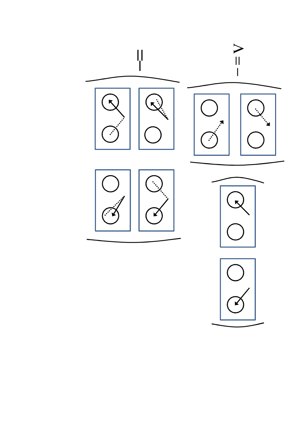
Figure 2: The matrix elements of W. The lines denote the matrix elements W⁡(x,y)W(x,y) in (22). An initial point and an end point of an arrow denote a row and a column respectively. We can obtain products of matrices by connecting arrows and integrating joint points on regions where the joint points exist. Instead of solid lines we use dotted lines for W−1W^{-1}.
Refer to caption
Figure 3: The diagrammatic calculation of Λ\Lambda in (23).
Refer to caption
Figure 4: The diagrammatic representations of Λ\Lambda in (25) and the identity in (24).
Refer to caption
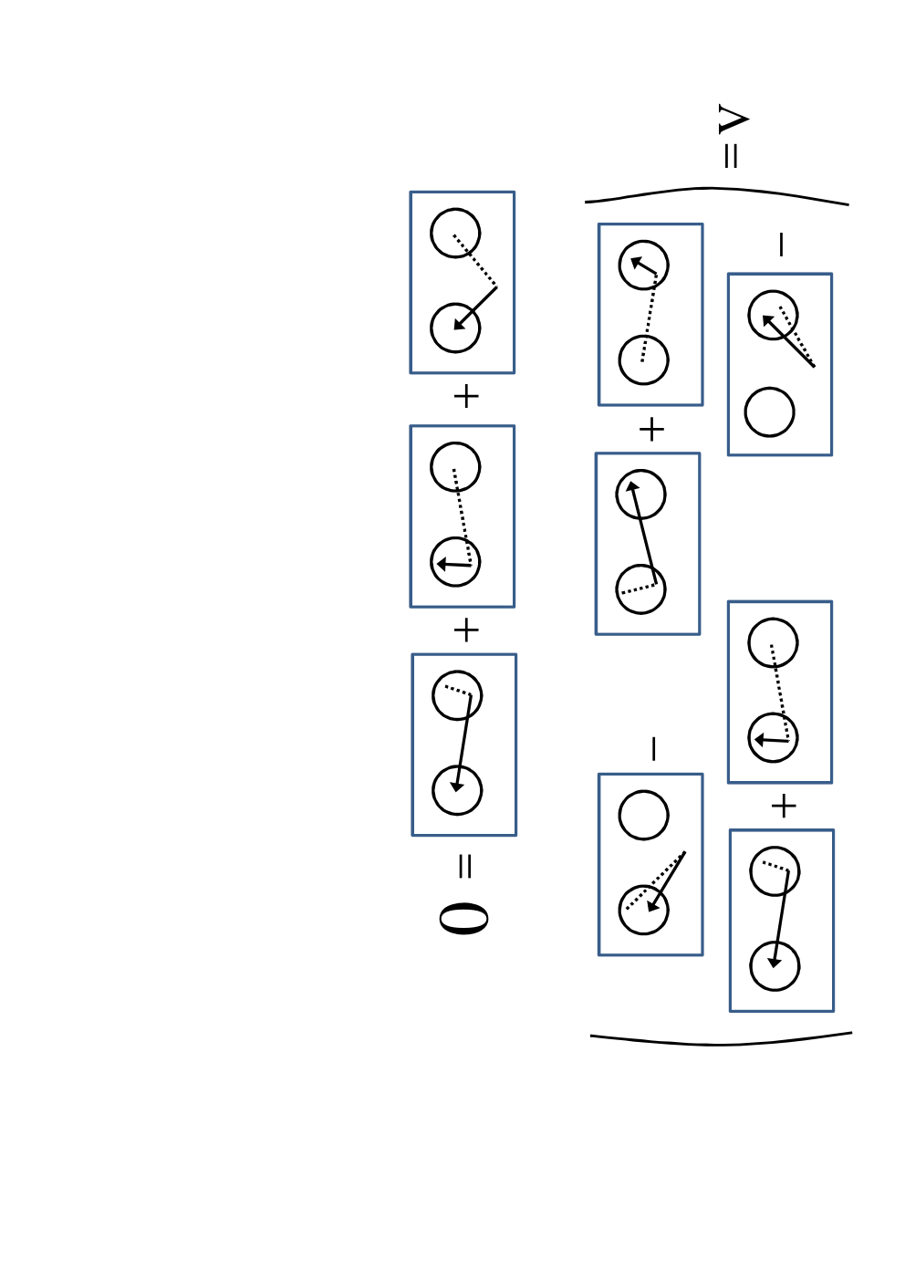
Figure 5: The diagrammatic representations of δ​Λ1\delta\Lambda_{1}, δ​Λ2\delta\Lambda_{2} and ΛD\Lambda_{D}.
Refer to caption
Figure 6: The diagrammatic representations of Λ0\Lambda^{0}, A0A^{0} and A0​δ​Λ1A^{0}\delta\Lambda_{1}.
Refer to caption
Figure 7: The diagrammatic calculation of δ​ΛD\delta\Lambda_{D} in (34).

Next, we obtain the rr dependence of Λ\Lambda by using (22). We represent the matrix elements of W⁡(W−1)W(W^{-1}) diagrammatically in Fig 2. Instead of solid lines we use dotted lines for W−1W^{-1}. The lines denote the matrix elements W⁡(x,y)W(x,y)(or W−1​(x,y)W^{-1}(x,y)) in (22). An initial point and an end point of an arrow denote a row and a column respectively. We can obtain products of matrices by connecting arrows and integrating joint points on regions where the joint points exist. We label coordinates in A,BA,B and CC as xa,xbx_{a},x_{b} and xcx_{c}. Then, from Fig 3 we obtain Λ=−E​BT\Lambda=-EB^{T} as

Λ=(Λ⁡(xa,ya)Λ⁡(xa,yb)Λ⁡(xb,ya)Λ⁡(xb,yb))=−(W−1​(xa,zc)W−1​(xb,zc))​(W⁡(zc,ya)W⁡(zc,yb))=−(∫Cdd​zc​W−1​(xa,zc)​W​(zc,ya)∫Cdd​zc​W−1​(xa,zc)​W​(zc,yb)∫Cdd​zc​W−1​(xb,zc)​W​(zc,ya)∫Cdd​zc​W−1​(xb,zc)​W​(zc,yb)).\begin{split}\Lambda&=\begin{pmatrix}\Lambda(x_{a},y_{a})&\Lambda(x_{a},y_{b})\\ \Lambda(x_{b},y_{a})&\Lambda(x_{b},y_{b})\end{pmatrix}=-\begin{pmatrix}W^{-1}(x_{a},z_{c})\\ W^{-1}(x_{b},z_{c})\end{pmatrix}\begin{pmatrix}W(z_{c},y_{a})&W(z_{c},y_{b})\end{pmatrix}\\ &=-\begin{pmatrix}\int_{C}d^{d}z_{c}W^{-1}(x_{a},z_{c})W(z_{c},y_{a})&\int_{C}d^{d}z_{c}W^{-1}(x_{a},z_{c})W(z_{c},y_{b})\\ \int_{C}d^{d}z_{c}W^{-1}(x_{b},z_{c})W(z_{c},y_{a})&\int_{C}d^{d}z_{c}W^{-1}(x_{b},z_{c})W(z_{c},y_{b})\end{pmatrix}.\end{split} (23)

To make the rr dependence of the non-diagonal elements of Λ\Lambda clear, we use the following identity,

∫A+B+Cdd​z​W−1​(xa,z)​W​(z,yb)=δ⁡(xa−yb)=0.\int_{A+B+C}d^{d}zW^{-1}(x_{a},z)W(z,y_{b})=\delta(x_{a}-y_{b})=0. (24)

We represent this identity diagrammatically in Fig 4. From (23) and (24) we obtain (see Fig 4)

Λ⁡(xa,yb)=∫Add​za​W−1​(xa,za)​W​(za,yb)+∫Bdd​zb​W−1​(xa,zb)​W​(zb,yb)Λ⁡(xb,ya)=∫Add​za​W−1​(xb,za)​W​(za,ya)+∫Bdd​zb​W−1​(xb,zb)​W​(zb,ya).\begin{split}&\Lambda(x_{a},y_{b})=\int_{A}d^{d}z_{a}W^{-1}(x_{a},z_{a})W(z_{a},y_{b})+\int_{B}d^{d}z_{b}W^{-1}(x_{a},z_{b})W(z_{b},y_{b})\\ &\Lambda(x_{b},y_{a})=\int_{A}d^{d}z_{a}W^{-1}(x_{b},z_{a})W(z_{a},y_{a})+\int_{B}d^{d}z_{b}W^{-1}(x_{b},z_{b})W(z_{b},y_{a}).\end{split} (25)

Note that from (22) W⁡(x,y)W(x,y) and W−1​(x,y)W^{-1}(x,y) have the different ‖x−y‖\|x-y\| dependence. So, from (23) and (25) we decompose Λ\Lambda as

Λ=ΛD+δ​Λ1+δ​Λ2\Lambda=\Lambda_{D}+\delta\Lambda_{1}+\delta\Lambda_{2} (26)

where we define (see Fig 5)

ΛD≡(Λ⁡(xa,ya)00Λ⁡(xb,yb)),\displaystyle\Lambda_{D}\equiv\begin{pmatrix}\Lambda(x_{a},y_{a})&0\\ 0&\Lambda(x_{b},y_{b})\end{pmatrix}, (27)
δ​Λ1≡(0∫Bdd​zb​W−1​(xa,zb)​W​(zb,yb)∫Add​za​W−1​(xb,za)​W​(za,ya)0),\displaystyle\delta\Lambda_{1}\equiv\begin{pmatrix}0&\int_{B}d^{d}z_{b}W^{-1}(x_{a},z_{b})W(z_{b},y_{b})\\ \int_{A}d^{d}z_{a}W^{-1}(x_{b},z_{a})W(z_{a},y_{a})&0\end{pmatrix}, (28)
δ​Λ2≡(0∫Add​za​W−1​(xa,za)​W​(za,yb)∫Bdd​zb​W−1​(xb,zb)​W​(zb,ya)0).\displaystyle\delta\Lambda_{2}\equiv\begin{pmatrix}0&\int_{A}d^{d}z_{a}W^{-1}(x_{a},z_{a})W(z_{a},y_{b})\\ \int_{B}d^{d}z_{b}W^{-1}(x_{b},z_{b})W(z_{b},y_{a})&0\end{pmatrix}. (29)

We approximate W⁡(xa,yb)≈Adrd+1W(x_{a},y_{b})\approx\tfrac{A_{d}}{r^{d+1}} and W−1​(xa,yb)≈Bdrd−1W^{-1}(x_{a},y_{b})\approx\tfrac{B_{d}}{r^{d-1}} because r≫R1,R2r\gg R_{1},R_{2}. Then we have

δ​Λ1≈Bdrd−1​(0∫Bdd​zb​W​(zb,yb)∫Add​za​W​(za,ya)0),\displaystyle\delta\Lambda_{1}\approx\dfrac{B_{d}}{r^{d-1}}\begin{pmatrix}0&\int_{B}d^{d}z_{b}W(z_{b},y_{b})\\ \int_{A}d^{d}z_{a}W(z_{a},y_{a})&0\end{pmatrix}, (30)
δ​Λ2≈Adrd+1​(0∫Add​za​W−1​(xa,za)∫Bdd​zb​W−1​(xb,zb)0).\displaystyle\delta\Lambda_{2}\approx\dfrac{A_{d}}{r^{d+1}}\begin{pmatrix}0&\int_{A}d^{d}z_{a}W^{-1}(x_{a},z_{a})\\ \int_{B}d^{d}z_{b}W^{-1}(x_{b},z_{b})&0\end{pmatrix}. (31)

Next we consider the non-perturbative part Λ0=limr→∞Λ\Lambda^{0}=\lim_{r\rightarrow\infty}\Lambda. From (30) and (31) we can see that δ​Λ1\delta\Lambda_{1} and δ​Λ2\delta\Lambda_{2} become 00 when r→∞r\rightarrow\infty. Note that the integral region of the integral in Λ⁡(xa,ya)\Lambda(x_{a},y_{a}) (Λ⁡(xb,yb)\Lambda(x_{b},y_{b})) become Ac≡ℝd−AA^{c}\equiv\mathbb{R}^{d}-A (Bc≡ℝd−BB^{c}\equiv\mathbb{R}^{d}-B) when r→∞r\rightarrow\infty, then we obtain (see Fig 6)

Λ0=−(∫Acdd​z​W−1​(xa,z)​W​(z,ya)00∫Bcdd​z​W−1​(xb,z)​W​(z,yb)).\Lambda^{0}=-\begin{pmatrix}\int_{A^{c}}d^{d}zW^{-1}(x_{a},z)W(z,y_{a})&0\\ 0&\int_{B^{c}}d^{d}zW^{-1}(x_{b},z)W(z,y_{b})\end{pmatrix}. (32)

From (32) we rewrite (26) as follows,

Λ=Λ0+δ​Λ1+δ​Λ2+δ​ΛD,\Lambda=\Lambda^{0}+\delta\Lambda_{1}+\delta\Lambda_{2}+\delta\Lambda_{D}, (33)

where we define (see Fig 7)

δ​ΛD≡ΛD−Λ0=(∫Bdd​zb​W−1​(xa,zb)​W​(zb,ya)00∫Add​za​W−1​(xb,za)​W​(za,yb)).\delta\Lambda_{D}\equiv\Lambda_{D}-\Lambda^{0}=\begin{pmatrix}\int_{B}d^{d}z_{b}W^{-1}(x_{a},z_{b})W(z_{b},y_{a})&0\\ 0&\int_{A}d^{d}z_{a}W^{-1}(x_{b},z_{a})W(z_{a},y_{b})\end{pmatrix}. (34)

We use the same approximation as we used in (30) and (31), then we obtain

δ​ΛD≈Ad​Bdr2​d​(∫Bdd​zb00∫Add​za).\delta\Lambda_{D}\approx\dfrac{A_{d}B_{d}}{r^{2d}}\begin{pmatrix}\int_{B}d^{d}z_{b}&0\\ 0&\int_{A}d^{d}z_{a}\end{pmatrix}. (35)

When we perform the perturbative calculation to obtain λm​(r)\lambda_{m}(r) which is the eigenvalues of Λ\Lambda, from (30), (31), (33) and (35) we can neglect δ​ΛD\delta\Lambda_{D} because it is higher order than δ​Λ1\delta\Lambda_{1} and δ​Λ2\delta\Lambda_{2} with respect to 1/r1/r. And we can neglect δ​Λ2\delta\Lambda_{2} because its nonzero matrix elements are in the same position as δ​Λ1\delta\Lambda_{1} and δ​Λ2\delta\Lambda_{2} is higher order than δ​Λ1\delta\Lambda_{1} with respect to 1/r1/r.

Because Λ\Lambda is not a symmetric matrix, in the later perturbative calculation we need A0​δ​Λ1A^{0}\delta\Lambda_{1} where A0A^{0} is defined as (see Fig 6)

A0≡limr→∞A=(W⁡(xa,ya)00W⁡(xb,yb)).A^{0}\equiv\lim_{r\rightarrow\infty}A=\begin{pmatrix}W(x_{a},y_{a})&0\\ 0&W(x_{b},y_{b})\end{pmatrix}. (36)

From (28), (30) and (36) we obtain (see Fig 6)

A0​δ​Λ1=(0∫Add​za​∫Bdd​zb​W​(xa,za)​W−1​(za,zb)​W​(zb,yb)∫Bdd​zb​∫Add​za​W​(xb,zb)​W−1​(zb,za)​W​(za,ya)0)≈Bdrd−1​(0∫Add​za​W​(xa,za)​∫Bdd​zb​W​(zb,yb)∫Bdd​zb​W​(xb,zb)​∫Add​za​W​(za,ya)0).\begin{split}A^{0}\delta\Lambda_{1}&=\begin{pmatrix}0&\int_{A}d^{d}z_{a}\int_{B}d^{d}z_{b}W(x_{a},z_{a})W^{-1}(z_{a},z_{b})W(z_{b},y_{b})\\ \int_{B}d^{d}z_{b}\int_{A}d^{d}z_{a}W(x_{b},z_{b})W^{-1}(z_{b},z_{a})W(z_{a},y_{a})&0\end{pmatrix}\\ &\approx\dfrac{B_{d}}{r^{d-1}}\begin{pmatrix}0&\int_{A}d^{d}z_{a}W(x_{a},z_{a})\int_{B}d^{d}z_{b}W(z_{b},y_{b})\\ \int_{B}d^{d}z_{b}W(x_{b},z_{b})\int_{A}d^{d}z_{a}W(z_{a},y_{a})&0\end{pmatrix}.\end{split} (37)

We have finished the first step.

Next, we calculate λm​(r)\lambda_{m}(r) by perturbation theory. This is almost similar to the time-independent perturbation theory with degeneracy of quantum mechanics. The only difference is that Λ\Lambda is not a symmetric matrix and A​ΛA\Lambda is a symmetric matrix.

We can approximate Λ≈Λ0+δ​Λ1\Lambda\approx\Lambda^{0}+\delta\Lambda_{1} and regard δ​Λ1\delta\Lambda_{1} as the perturbative part. Then, from (30) we expand λm​(r)\lambda_{m}(r) with respect to 1/rd−11/r^{d-1}. We expand λm\lambda_{m} around λm0≡λm​(r=∞)\lambda_{m}^{0}\equiv\lambda_{m}(r=\infty),

λm=λm0+δ​λm1+δ​λm2,\lambda_{m}=\lambda_{m}^{0}+\delta\lambda_{m}^{1}+\delta\lambda_{m}^{2}, (38)

where δ​λm1\delta\lambda_{m}^{1} and δ​λm2\delta\lambda_{m}^{2} are the first and the second order perturbations.

Next we substitute (38) into (12),

SA​B​(r,R1,R2)=∑mf⁡(λm)=SA​(R1)+SB​(R2)+∑m[δ​λm​d​fd​λm|λm=λm0+12​(δ​λm)2​d2​fd​λm2|λm=λm0],\begin{split}S_{AB}(r,R_{1},R_{2})&=\sum_{m}f(\lambda_{m})\\ &=S_{A}(R_{1})+S_{B}(R_{2})+\sum_{m}\left[\delta\lambda_{m}\left.\dfrac{df}{d\lambda_{m}}\right|_{\lambda_{m}=\lambda_{m}^{0}}+\dfrac{1}{2}(\delta\lambda_{m})^{2}\left.\dfrac{d^{2}f}{d\lambda_{m}^{2}}\right|_{\lambda_{m}=\lambda_{m}^{0}}\right],\end{split} (39)

where δ​λm≡δ​λm1+δ​λm2\delta\lambda_{m}\equiv\delta\lambda_{m}^{1}+\delta\lambda_{m}^{2}. We will show that the first order perturbation in (39) (i.e ∑mδ​λm1​d​fd​λm|λm=λm0\sum_{m}\delta\lambda_{m}^{1}\left.\dfrac{df}{d\lambda_{m}}\right|_{\lambda_{m}=\lambda_{m}^{0}}) is zero, so we must calculate the second order perturbations.

We label the λm0\lambda_{m}^{0}’s as λm0>λn0​when​m>n\lambda_{m}^{0}>\lambda_{n}^{0}~\textrm{when}~m>n. And we define the eigenvectors of Λ0\Lambda^{0},

fm​1​α0=(fm​1​α0​(xa)0),fn​2​β0=(0fn​2​β0​(xb)),Λ0​fm​1​α0=λm0​fm​1​α0,Λ0​fm​2​β0=λm0​fm​2​β0,f_{m1\alpha}^{0}=\begin{pmatrix}f_{m1\alpha}^{0}(x_{a})\\ 0\end{pmatrix},f_{n2\beta}^{0}=\begin{pmatrix}0\\ f_{n2\beta}^{0}(x_{b})\end{pmatrix},\Lambda^{0}f_{m1\alpha}^{0}=\lambda_{m}^{0}f_{m1\alpha}^{0},\Lambda^{0}f_{m2\beta}^{0}=\lambda_{m}^{0}f_{m2\beta}^{0}, (40)

where α=1,⋯,Mm\alpha=1,\cdots,M_{m} and β=1,⋯,Nn\beta=1,\cdots,N_{n} are the labels of the degeneracy. And we normalize fm​i​α0​(i=1,2)f_{mi\alpha}^{0}~~(i=1,2) as follow,

fm​i​α0​T​A0​fn​j​β0=δm​n​δi​j​δα​β.f_{mi\alpha}^{0T}A^{0}f_{nj\beta}^{0}=\delta_{mn}\delta_{ij}\delta_{\alpha\beta}. (41)

This normalization is always possible because A0A^{0} is a positive definite symmetric matrix. For general R1R_{1} and R2R_{2}, Λ01\Lambda^{01} and Λ02\Lambda^{02} have different eigenvalues, so there are two groups of λm0\lambda_{m}^{0}; one is the group of the common eigenvalues of Λ01\Lambda^{01} and Λ02\Lambda^{02}, the other is not. We will see that δ​λm1\delta\lambda_{m}^{1} of the latter group are zero. We expand fm​γf_{m\gamma} which is the eigenvector of Λ\Lambda in the following way,

fm​γ=∑αaγ​α​fm​1​α0+∑βbγ​β​fm​2​β0+fm​γ1+fm​γ2≡ξm​γ0+fm​γ1+fm​γ2f_{m\gamma}=\sum_{\alpha}a_{\gamma\alpha}f_{m1\alpha}^{0}+\sum_{\beta}b_{\gamma\beta}f_{m2\beta}^{0}+f_{m\gamma}^{1}+f_{m\gamma}^{2}\equiv\xi_{m\gamma}^{0}+f_{m\gamma}^{1}+f_{m\gamma}^{2} (42)

where fm​γ1f_{m\gamma}^{1} and fm​γ2f_{m\gamma}^{2} are the first and the second order perturbations. Note that when λm0\lambda_{m}^{0} is an eigenvalue of Λ01\Lambda^{01} (Λ02\Lambda^{02}) and is not an eigenvalue of Λ02\Lambda^{02} (Λ01\Lambda^{01}), then the coefficients bγ​βb_{\gamma\beta} (aγ​αa_{\gamma\alpha}) are zero ; because the zeroth order eigenvectors fm​2​β0f_{m2\beta}^{0} (fm​1​α0f_{m1\alpha}^{0}) do not exist. So either the coefficients aγ​αa_{\gamma\alpha} or bγ​βb_{\gamma\beta} are zero when λm0\lambda_{m}^{0} is not a common eigenvalue of Λ01\Lambda^{01} and Λ02\Lambda^{02}. We substitute (42) into the eigenvalue equation (we approximate Λ≈Λ0+δ​Λ1\Lambda\approx\Lambda^{0}+\delta\Lambda_{1}) , then we have

(Λ0+δ​Λ1)​fm​γ=(λm0+δ​λm​γ1+δ​λm​γ2)​fm​γ.(\Lambda^{0}+\delta\Lambda_{1})f_{m\gamma}=(\lambda_{m}^{0}+\delta\lambda_{m\gamma}^{1}+\delta\lambda_{m\gamma}^{2})f_{m\gamma}. (43)

We obtain equations of the first and the second order perturbation.

Λ0​fm​γ1+δ​Λ1​ξm​γ0=λm0​fm​γ1+δ​λm​γ1​ξm​γ0,\displaystyle\Lambda^{0}f_{m\gamma}^{1}+\delta\Lambda_{1}\xi_{m\gamma}^{0}=\lambda_{m}^{0}f_{m\gamma}^{1}+\delta\lambda_{m\gamma}^{1}\xi_{m\gamma}^{0}, (44)
Λ0​fm​γ2+δ​Λ1​fm​γ1=λm0​fm​γ2+δ​λm​γ1​fm​γ1+δ​λm​γ2​ξm​γ0.\displaystyle\Lambda^{0}f_{m\gamma}^{2}+\delta\Lambda_{1}f_{m\gamma}^{1}=\lambda_{m}^{0}f_{m\gamma}^{2}+\delta\lambda_{m\gamma}^{1}f_{m\gamma}^{1}+\delta\lambda_{m\gamma}^{2}\xi_{m\gamma}^{0}. (45)

We multiply (44) by fm​j​γ′0​T​A0f_{mj\gamma^{\prime}}^{0T}A^{0} from the left . The first term of the left hand side of (44) cancel the first term of the right hand side of (44) because A0​Λ0A^{0}\Lambda^{0} is a symmetric matrix, then we obtain

∑αaγ​α​Vm​γ′​m​αj​1+∑βbγ​β​Vm​γ′​m​βj​2=δ​λm​γ1​(aγ​γ′​δj​1+bγ​γ′​δj​2),\displaystyle\sum_{\alpha}a_{\gamma\alpha}V_{m\gamma^{\prime}m\alpha}^{j1}+\sum_{\beta}b_{\gamma\beta}V_{m\gamma^{\prime}m\beta}^{j2}=\delta\lambda_{m\gamma}^{1}(a_{\gamma\gamma^{\prime}}\delta^{j1}+b_{\gamma\gamma^{\prime}}\delta^{j2}), (46)

where

Vm​α​n​βi​j≡fm​i​α0​T​A0​δ​Λ1​fn​j​β0.\displaystyle V_{m\alpha n\beta}^{ij}\equiv f_{mi\alpha}^{0T}A^{0}\delta\Lambda_{1}f_{nj\beta}^{0}. (47)

From (37) we obtain Vm​α​n​β11=Vm​α​n​β22=0V_{m\alpha n\beta}^{11}=V_{m\alpha n\beta}^{22}=0 and

Vm​α​n​β12=(fm​1​α0​(xa)0)​(A0​δ​Λ1​(xa,ya)A0​δ​Λ1​(xa,yb)A0​δ​Λ1​(xb,ya)A0​δ​Λ1​(xb,yb))​(0fn​2​β0​(yb))=Bdrd−1​∫Add​xa​∫Add​za​W​(xa,za)​fm​1​α0​(xa)​∫Bdd​yb​∫Bdd​zb​W​(yb,zb)​fn​2​β0​(yb)≡Bdrd−1​Cm​α​n​β\displaystyle\begin{split}V_{m\alpha n\beta}^{12}&=\begin{pmatrix}f_{m1\alpha}^{0}(x_{a})&0\end{pmatrix}\begin{pmatrix}A^{0}\delta\Lambda_{1}(x_{a},y_{a})&A^{0}\delta\Lambda_{1}(x_{a},y_{b})\\ A^{0}\delta\Lambda_{1}(x_{b},y_{a})&A^{0}\delta\Lambda_{1}(x_{b},y_{b})\end{pmatrix}\begin{pmatrix}0\\ f_{n2\beta}^{0}(y_{b})\end{pmatrix}\\ &=\dfrac{B_{d}}{r^{d-1}}\int_{A}d^{d}x_{a}\int_{A}d^{d}z_{a}W(x_{a},z_{a})f_{m1\alpha}^{0}(x_{a})\int_{B}d^{d}y_{b}\int_{B}d^{d}z_{b}W(y_{b},z_{b})f_{n2\beta}^{0}(y_{b})\equiv\dfrac{B_{d}}{r^{d-1}}C_{m\alpha n\beta}\end{split} (48)

and Vm​α​n​β12=Vn​β​m​α21V_{m\alpha n\beta}^{12}=V_{n\beta m\alpha}^{21}. We define an Mm×NnM_{m}\times N_{n} matrix Cm​nC_{mn} as (Cm​n)α​β=Cm​α​n​β(C_{mn})_{\alpha\beta}=C_{m\alpha n\beta} and write (46) as follows,

Bdrd−1​(0Cm​mCm​mT0)​(𝐚γ𝐛γ)=δ​λm​γ1​(𝐚γ𝐛γ)\dfrac{B_{d}}{r^{d-1}}\begin{pmatrix}0&C_{mm}\\ C_{mm}^{T}&0\end{pmatrix}\begin{pmatrix}\mathbf{a}_{\gamma}\\ \mathbf{b}_{\gamma}\end{pmatrix}=\delta\lambda_{m\gamma}^{1}\begin{pmatrix}\mathbf{a}_{\gamma}\\ \mathbf{b}_{\gamma}\end{pmatrix} (49)

where (𝐚γ)α=aγ​α(\mathbf{a}_{\gamma})_{\alpha}=a_{\gamma\alpha} and (𝐛γ)β=bγ​β(\mathbf{b}_{\gamma})_{\beta}=b_{\gamma\beta}. From (49), if λm0\lambda_{m}^{0} is not a common eigenvalue of Λ01\Lambda^{01} and Λ02\Lambda^{02}, δ​λm​γ1\delta\lambda_{m\gamma}^{1} is zero; because either aγ​αa_{\gamma\alpha} or bγ​βb_{\gamma\beta} are zero when λm0\lambda_{m}^{0} is not a common eigenvalue of Λ01\Lambda^{01} and Λ02\Lambda^{02}. We first consider the case that Mm≥NmM_{m}\geq N_{m}. In this case we obtain the following eigenvalue equation [17].

det|x​1Mm×Mm−Cm​m−Cm​mTx​1Nm×Nm|=det(x​1Mm×Mm)​det(x​1Nm×Nm−x−1​Cm​mT​Cm​m)=xMm−Nm​det(x2​1Nm×Nm−Cm​mT​Cm​m)=0.\begin{split}\det\begin{vmatrix}x1_{M_{m}\times M_{m}}&-C_{mm}\\ -C_{mm}^{T}&x1_{N_{m}\times N_{m}}\end{vmatrix}&=\det(x1_{M_{m}\times M_{m}})\det(x1_{N_{m}\times N_{m}}-x^{-1}C_{mm}^{T}C_{mm})\\ &=x^{M_{m}-N_{m}}\det(x^{2}1_{N_{m}\times N_{m}}-C_{mm}^{T}C_{mm})=0.\end{split} (50)

We define the eigenvalues of Cm​mT​Cm​mC_{mm}^{T}C_{mm} as cm​α(α=1,⋯Mm)c_{m\alpha}~~~(\alpha=1,\cdots M_{m}). Cm​mT​Cm​mC_{mm}^{T}C_{mm} is a positive semidefinite matrix because Cm​mC_{mm} is a real matrix, so cm​α≥0c_{m\alpha}\geq 0. Then we obtain δ​λm​γ1\delta\lambda_{m\gamma}^{1} from (49) and (50) .

δ​λm​γ1={0±Bdrd−1​cm​α(α=1,⋯Mm).\delta\lambda_{m\gamma}^{1}=\begin{cases}0&\\ \pm\dfrac{B_{d}}{r^{d-1}}\sqrt{c_{m\alpha}}&(\alpha=1,\cdots M_{m})\end{cases}. (51)

When Mm<NmM_{m}<N_{m}, we can obtain δ​λm​γ1\delta\lambda_{m\gamma}^{1} in the same way. We define the eigenvalues of Cm​m​Cm​mTC_{mm}C_{mm}^{T} as dm​α(≥0)(α=1,⋯Nm)d_{m\alpha}(\geq 0)~~~(\alpha=1,\cdots N_{m}). Then we obtain

δ​λm​γ1={0±Bdrd−1​dm​α(α=1,⋯Nm).\delta\lambda_{m\gamma}^{1}=\begin{cases}0&\\ \pm\dfrac{B_{d}}{r^{d-1}}\sqrt{d_{m\alpha}}&(\alpha=1,\cdots N_{m})\end{cases}. (52)

Then ∑m,γδ​λm​γ1​d​fd​λm|λm=λm0=0\sum_{m,\gamma}\delta\lambda_{m\gamma}^{1}\left.\dfrac{df}{d\lambda_{m}}\right|_{\lambda_{m}=\lambda_{m}^{0}}=0, because we have ∑γδ​λm​γ1=0\sum_{\gamma}\delta\lambda_{m\gamma}^{1}=0 from (51) and (52).

Next we consider δ​λm​γ2\delta\lambda_{m\gamma}^{2}. We skip the detailed calculation because it is also almost similar to the time-independent perturbation theory with degeneracy of quantum mechanics. Then we can write δ​λm​γ2\delta\lambda_{m\gamma}^{2} as follows

δ​λm​γ2=∑n(≠m),i,β1λm0−λn0​(fn​i​β0​T​A0​δ​Λ1​ξm​γ0)​(ξm​γ0​T​A0​δ​Λ1​fn​i​β0)=∑n(≠m)1λm0−λn0​ξm​γ0​T​A0​δ​Λ1​ϕ^n​δ​Λ1​ξm​γ0\begin{split}\delta\lambda_{m\gamma}^{2}&=\sum_{n(\neq m),i,\beta}\dfrac{1}{\lambda_{m}^{0}-\lambda_{n}^{0}}(f_{ni\beta}^{0T}A^{0}\delta\Lambda_{1}\xi_{m\gamma}^{0})(\xi_{m\gamma}^{0T}A^{0}\delta\Lambda_{1}f_{ni\beta}^{0})\\ &=\sum_{n(\neq m)}\dfrac{1}{\lambda_{m}^{0}-\lambda_{n}^{0}}\xi_{m\gamma}^{0T}A^{0}\delta\Lambda_{1}\hat{\phi}_{n}\delta\Lambda_{1}\xi_{m\gamma}^{0}\end{split} (53)

where

ϕ^n≡∑i,βfn​i​β0​fn​i​β0​T​A0.\hat{\phi}_{n}\equiv\sum_{i,\beta}f_{ni\beta}^{0}f_{ni\beta}^{0T}A^{0}. (54)

ϕ^n\hat{\phi}_{n} is a projection operator on the eigenspace of λn0\lambda_{n}^{0}. To obtain δ​λm​γ2\delta\lambda_{m\gamma}^{2} we must obtain ξm​γ0\xi_{m\gamma}^{0} by solving the eigenvalue problem, but it is not necessary for our purpose because we want to know only ∑m,γδ​λm​γ2​d​fd​λm|λm=λm0\sum_{m,\gamma}\delta\lambda_{m\gamma}^{2}\left.\dfrac{df}{d\lambda_{m}}\right|_{\lambda_{m}=\lambda_{m}^{0}}. From (53) we obtain

∑m,γδ​λm​γ2​d​fd​λm|λm=λm0=∑m,γ∑n(≠m)1λm0−λn0​ξm​γ0​T​A0​δ​Λ1​ϕ^n​δ​Λ1​ξm​γ0​d​fd​λm|λm=λm0=∑m,n⁡(m≠n)1λm0−λn0​T​r​(ϕ^m​δ​Λ1​ϕ^n​δ​Λ1)​d​fd​λm|λm=λm0=∑m,n⁡(m>n)1λm0−λn0​T​r​(ϕ^m​δ​Λ1​ϕ^n​δ​Λ1)​(d​fd​λm|λm=λm0−d​fd​λn|λn=λn0).\begin{split}\sum_{m,\gamma}\delta\lambda_{m\gamma}^{2}\left.\dfrac{df}{d\lambda_{m}}\right|_{\lambda_{m}=\lambda_{m}^{0}}&=\sum_{m,\gamma}\sum_{n(\neq m)}\dfrac{1}{\lambda_{m}^{0}-\lambda_{n}^{0}}\xi_{m\gamma}^{0T}A^{0}\delta\Lambda_{1}\hat{\phi}_{n}\delta\Lambda_{1}\xi_{m\gamma}^{0}\left.\dfrac{df}{d\lambda_{m}}\right|_{\lambda_{m}=\lambda_{m}^{0}}\\ &=\sum_{m,n(m\neq n)}\dfrac{1}{\lambda_{m}^{0}-\lambda_{n}^{0}}Tr(\hat{\phi}_{m}\delta\Lambda_{1}\hat{\phi}_{n}\delta\Lambda_{1})\left.\dfrac{df}{d\lambda_{m}}\right|_{\lambda_{m}=\lambda_{m}^{0}}\\ &=\sum_{m,n(m>n)}\dfrac{1}{\lambda_{m}^{0}-\lambda_{n}^{0}}Tr(\hat{\phi}_{m}\delta\Lambda_{1}\hat{\phi}_{n}\delta\Lambda_{1})\left(\left.\dfrac{df}{d\lambda_{m}}\right|_{\lambda_{m}=\lambda_{m}^{0}}-\left.\dfrac{df}{d\lambda_{n}}\right|_{\lambda_{n}=\lambda_{n}^{0}}\right).\end{split} (55)

In the second line we have used

∑γξm​γ0​ξm​γ0​T​A0=ϕ^m,\sum_{\gamma}\xi_{m\gamma}^{0}\xi_{m\gamma}^{0T}A^{0}=\hat{\phi}_{m}, (56)

and in the third line we have used cyclic property of trace. Next we examine the sign of (55). Its trace term is positive because

T​r​(ϕ^m​δ​Λ1​ϕ^n​δ​Λ1)=∑i,α,j,β(fn​i​α0​T​A0​δ​Λ1​fm​j​β0)​(fm​j​β0​T​A0​δ​Λ1​fn​i​α0)=∑i,α,j,βVn​α​m​βi​j​Vm​β​n​αj​i=∑i,α,j,β(Vn​α​m​βi​j)2=2​(Bdrd−1)2​∑α,β(Cm​α​n​β)2≥0.\begin{split}Tr(\hat{\phi}_{m}\delta\Lambda_{1}\hat{\phi}_{n}\delta\Lambda_{1})&=\sum_{i,\alpha,j,\beta}(f_{ni\alpha}^{0T}A^{0}\delta\Lambda_{1}f_{mj\beta}^{0})(f_{mj\beta}^{0T}A^{0}\delta\Lambda_{1}f_{ni\alpha}^{0})\\ &=\sum_{i,\alpha,j,\beta}V_{n\alpha m\beta}^{ij}V_{m\beta n\alpha}^{ji}=\sum_{i,\alpha,j,\beta}(V_{n\alpha m\beta}^{ij})^{2}=2\left(\dfrac{B_{d}}{r^{d-1}}\right)^{2}\sum_{\alpha,\beta}(C_{m\alpha n\beta})^{2}\geq 0.\end{split} (57)

And from (12) we obtain

d​fd​λ\displaystyle\dfrac{df}{d\lambda} =12​1+λ​ln⁡[1+1λ+1λ]>0​for​λ>0,\displaystyle=\dfrac{1}{2\sqrt{1+\lambda}}\ln\left[\sqrt{1+\dfrac{1}{\lambda}}+\dfrac{1}{\sqrt{\lambda}}\right]>0~~~\textrm{for}~~\lambda>0, (58)
d2​fd​λ2\displaystyle\dfrac{d^{2}f}{d\lambda^{2}} =−14​1+λ​[11+λ​ln⁡[1+1λ+1λ]+1λ​1+λ]<0​for​λ>0.\displaystyle=-\dfrac{1}{4\sqrt{1+\lambda}}\left[\dfrac{1}{1+\lambda}\ln\left[\sqrt{1+\dfrac{1}{\lambda}}+\dfrac{1}{\sqrt{\lambda}}\right]+\dfrac{1}{\lambda\sqrt{1+\lambda}}\right]<0~~~\textrm{for}~~\lambda>0. (59)

From (57), (59) and λm0>λn0​(m>n)\lambda_{m}^{0}>\lambda_{n}^{0}~~(m>n) , (55) is negative. And from (59) we obtain

∑m,γ(δ​λm​γ1)2​d2​fd​λm2|λm=λm0≤0.\sum_{m,\gamma}(\delta\lambda_{m\gamma}^{1})^{2}\left.\dfrac{d^{2}f}{d\lambda_{m}^{2}}\right|_{\lambda_{m}=\lambda_{m}^{0}}\leq 0. (60)

Finally, from (39), (51), (52), (55) and (57) we obtain

SA​B​(r,R1,R2)−SA​(R1)−SB​(R2)=∑m,γ[δ​λm​γ2​d​fd​λm|λm=λm0+12​(δ​λm1)2​d2​fd​λm2|λm=λm0]=(Bdrd−1)2[∑m,n⁡(m>n)2λm0−λn0∑α,β(Cm​α​n​β)2(d​fd​λm|λm=λm0−d​fd​λn|λn=λn0)+∑m′,αcm′​αd2​fd​λm2|λm=λm′0+∑m′′,αdm′′​αd2​fd​λm2|λm=λm′′0]≡1r2​d−2G(R1,R2)≤0\begin{split}&S_{AB}(r,R_{1},R_{2})-S_{A}(R_{1})-S_{B}(R_{2})=\sum_{m,\gamma}\left[\delta\lambda_{m\gamma}^{2}\left.\dfrac{df}{d\lambda_{m}}\right|_{\lambda_{m}=\lambda_{m}^{0}}+\dfrac{1}{2}(\delta\lambda_{m}^{1})^{2}\left.\dfrac{d^{2}f}{d\lambda_{m}^{2}}\right|_{\lambda_{m}=\lambda_{m}^{0}}\right]\\ &=\left(\dfrac{B_{d}}{r^{d-1}}\right)^{2}\Bigl[\sum_{m,n(m>n)}\dfrac{2}{\lambda_{m}^{0}-\lambda_{n}^{0}}\sum_{\alpha,\beta}(C_{m\alpha n\beta})^{2}\left(\left.\dfrac{df}{d\lambda_{m}}\right|_{\lambda_{m}=\lambda_{m}^{0}}-\left.\dfrac{df}{d\lambda_{n}}\right|_{\lambda_{n}=\lambda_{n}^{0}}\right)\\ &+\sum_{m^{\prime},\alpha}c_{m^{\prime}\alpha}\left.\dfrac{d^{2}f}{d\lambda_{m}^{2}}\right|_{\lambda_{m}=\lambda_{m^{\prime}}^{0}}+\sum_{m^{\prime\prime},\alpha}d_{m^{\prime\prime}\alpha}\left.\dfrac{d^{2}f}{d\lambda_{m}^{2}}\right|_{\lambda_{m}=\lambda_{m^{\prime\prime}}^{0}}\Bigr]\equiv\dfrac{1}{r^{2d-2}}G(R_{1},R_{2})\leq 0\end{split} (61)

where ∑m′\sum_{m^{\prime}} denotes the summation taken over the common eigenvalues of Λ01\Lambda^{01} and Λ02\Lambda^{02}, whose degeneracy is Mm≥NmM_{m}\geq N_{m}, and ∑m′′\sum_{m^{\prime\prime}} denotes the summation taken over the common eigenvalues of Λ01\Lambda^{01} and Λ02\Lambda^{02}, whose degeneracy is Mm<NmM_{m}<N_{m}.

We have obtained the rr dependence of SC​(r,R1,R2)=SA​B​(r,R1,R2)S_{C}(r,R_{1},R_{2})=S_{AB}(r,R_{1},R_{2}) in (61), then we next consider G⁡(R1,R2)G(R_{1},R_{2}). To calculate G⁡(R1,R2)G(R_{1},R_{2}) we need to know λm0\lambda_{m}^{0} and fm​i​α0f_{mi\alpha}^{0} which we do not examine in this paper. But from Cm​α​n​β​(R1=0,R2)=Cm​α​n​β​(R1,R2=0)=0C_{m\alpha n\beta}(R_{1}=0,R_{2})=C_{m\alpha n\beta}(R_{1},R_{2}=0)=0 we obtain a trivial property of G⁡(R1,R2)G(R_{1},R_{2}),

G⁡(R1=0,R2)=G⁡(R1,R2=0)=0.G(R_{1}=0,R_{2})=G(R_{1},R_{2}=0)=0. (62)

And G⁡(R1,R2)G(R_{1},R_{2}) depends on the cutoff length ll because λm0,fm​i​α0\lambda_{m}^{0}~,~f_{mi\alpha}^{0} and Cm​α​n​βC_{m\alpha n\beta} depend on ll. (λm0\lambda_{m}^{0} are dimensionless, so they depend on R1/lR_{1}/l or R2/lR_{2}/l. And in (48) ∫Add​za​W​(xa,za)\int_{A}d^{d}z_{a}W(x_{a},z_{a}) and ∫Bdd​zb​W​(yb,zb)\int_{B}d^{d}z_{b}W(y_{b},z_{b}) depend on ll because W⁡(x,y)W(x,y) depend on ll for x≈yx\approx y, so Cm​α​n​βC_{m\alpha n\beta} depends on ll. ) Probably G⁡(R1,R2)G(R_{1},R_{2}) diverges when l→0l\rightarrow 0, as SA​(R1)S_{A}(R_{1}) and SB​(R2)S_{B}(R_{2}) have 1/ld−11/l^{d-1} divergence [1, 2]. And G⁡(R1,R2)G(R_{1},R_{2}) most likely diverges more weakly than SA​(R1)S_{A}(R_{1}) and SB​(R2)S_{B}(R_{2}). Then, by dimensional analysis, when R1=R2≡RR_{1}=R_{2}\equiv R we can assume

G⁡(R1=R,R2=R)=g​R2​d−2​(Rl)m​(ln⁡(Rl))nd−1≥m≥0,n≥0,g<0G(R_{1}=R,R_{2}=R)=gR^{2d-2}\left(\dfrac{R}{l}\right)^{m}\left(\ln\left(\dfrac{R}{l}\right)\right)^{n}~~~~d-1\geq m\geq 0,n\geq 0,g<0 (63)

where gg is a dimensionless constant.

Finally we consider the condition under which the approximations are good. When r≫R1,R2r\gg R_{1},R_{2},   δ​Λ≈δ​Λ1\delta\Lambda\approx\delta\Lambda_{1} is a good approximation. When |Bdrd−1​Cm​α​n​β|≪|λm0−λn0||\dfrac{B_{d}}{r^{d-1}}C_{m\alpha n\beta}|\ll|\lambda_{m}^{0}-\lambda_{n}^{0}|, the perturbation theory is a good approximation. The latter condition might have ll dependence, so we might need the condition R/r≪(l/R)aR/r\ll(l/R)^{a}, where a≥0a\geq 0.

Refer to caption
Figure 8: The diagrammatic representations of Λ~D\tilde{\Lambda}_{D}, A~\tilde{A} and δ​Λ~D\delta\tilde{\Lambda}_{D}.

V entanglement entropy of two black holes in a d+1d+1 dimensional massless free scalar field

In this section we consider the entanglement entropy of the massless free scalar field on the outside region CC of two black holes AA and BB whose radii are R1R_{1} and R2R_{2}. The action of the massless free scalar field is given by

S=−12∫ddx−ggμ​ν∇μϕ∇νϕ.S=-\dfrac{1}{2}\int d^{d}x\sqrt{-g}g^{\mu\nu}\nabla_{\mu}\phi\nabla_{\nu}\phi. (64)

First we specify the vacuum state of the scalar field. The vacuum state is specified by specifying the time coordinate tt. We use the coordinate system which have following properties: this coordinate system covers the inside and the outside regions of two black holes and does not have the coordinate singularity on the horizons and becomes the orthogonal coordinate system of Minkowski spacetime in the region far from the two black holes. To construct this coordinate system, we use the coordinates which is similar to the Kruskal coordinates in the inside regions and the neighborhood of black holes, and similar to the Schwarzschild coordinates in the other region. In this coordinate system gt​tg^{tt} is positive everywhere, then from (64) GM​NG_{MN} and VM​NV_{MN} in (5) are positive definite. So we can use the formalism in the Section III.

We can use the method of the last section with some modifications. In the black hole case W⁡(x,y)W(x,y) and W−1​(x,y)W^{-1}(x,y) depend on rr, so we write them as W⁡(x,y,r)W(x,y;r) and W−1​(x,y,r)W^{-1}(x,y;r). Exactly in the same way as in Minkowski spacetime, Eqs. (26)-(29) hold because (24) holds. On the other hand Λ0(=limr→∞Λ)\Lambda_{0}(=\lim_{r\rightarrow\infty}\Lambda) changes because W⁡(x,y,r)W(x,y;r) and W−1​(x,y,r)W^{-1}(x,y;r) depend on rr. We define WA​(x,y)W_{A}(x,y) and WA−1​(x,y)W_{A}^{-1}(x,y)(WB​(x,y)W_{B}(x,y) and WB−1​(x,y)W_{B}^{-1}(x,y)) as W⁡(x,y)W(x,y) and W−1​(x,y)W^{-1}(x,y) in the case that the only one black hole AA(BB) exists. Then we have

Λ0=−(∫Acdd​z​WA−1​(xa,z)​WA​(z,ya)00∫Bcdd​z​WB−1​(xb,z)​WB​(z,yb)).\Lambda^{0}=-\begin{pmatrix}\int_{A^{c}}d^{d}zW_{A}^{-1}(x_{a},z)W_{A}(z,y_{a})&0\\ 0&\int_{B^{c}}d^{d}zW_{B}^{-1}(x_{b},z)W_{B}(z,y_{b})\end{pmatrix}. (65)

It is difficult to evaluate the rr dependence of δ​ΛD=ΛD−Λ0\delta\Lambda_{D}=\Lambda_{D}-\Lambda^{0} because it is difficult to evaluate W⁡(x,y,r)−WA⁡(B)​(x,y)W(x,y;r)-W_{A(B)}(x,y) and W−1​(x,y,r)−WA⁡(B)−1​(x,y)W^{-1}(x,y;r)-W^{-1}_{A(B)}(x,y). So, in the black hole case we do not consider Λ0\Lambda_{0} as the non-perturbative part. Instead we define Λ~D​(r)\tilde{\Lambda}_{D}(r) and A~​(r)\tilde{A}(r) as (see Fig 8)

Λ~D​(r)≡(ΛA​(xa,ya,r)00ΛB​(xb,yb,r))\displaystyle\tilde{\Lambda}_{D}(r)\equiv\begin{pmatrix}\Lambda_{A}(x_{a},y_{a};r)&0\\ 0&\Lambda_{B}(x_{b},y_{b};r)\end{pmatrix}
≡(−∫AcddzW−1(xa,z;r)W(z,ya;r)00−∫BcddzW−1(xb,z;r)W(z,yb;r)),\displaystyle\equiv\begin{pmatrix}-\int_{A^{c}}d^{d}zW^{-1}(x_{a},z;r)W(z,y_{a};r)&0\\ 0&-\int_{B^{c}}d^{d}zW^{-1}(x_{b},z;r)W(z,y_{b};r)\end{pmatrix}, (66)
A~​(r)≡(W⁡(xa,ya,r)00W⁡(xb,yb,r)),\displaystyle\tilde{A}(r)\equiv\begin{pmatrix}W(x_{a},y_{a};r)&0\\ 0&W(x_{b},y_{b};r)\end{pmatrix}, (67)

and we consider Λ~D\tilde{\Lambda}_{D} as the non-perturbative part. Note that ΛA\Lambda_{A} and ΛB\Lambda_{B} are the matrices Λ\Lambda corresponding to SA​(r,R1,R2)S_{A}(r,R_{1},R_{2}) and SB​(r,R1,R2)S_{B}(r,R_{1},R_{2}). So we will obtain SA​BS_{AB} as the following form, SA​B​(r,R1,R2)=SA​(r,R1,R2)+SB​(r,R1,R2)+δ​SA​B​(r,R1,R2)S_{AB}(r,R_{1},R_{2})=S_{A}(r,R_{1},R_{2})+S_{B}(r,R_{1},R_{2})+\delta S_{AB}(r,R_{1},R_{2}). We calculate the leading term of δ​SA​B​(r,R1,R2)\delta S_{AB}(r,R_{1},R_{2}) with respect to 1/r1/r.

We define δ​Λ~D≡ΛD−Λ~D\delta\tilde{\Lambda}_{D}\equiv\Lambda_{D}-\tilde{\Lambda}_{D} (see Fig 8), then we have Λ=Λ~D+δ​Λ1+δ​Λ2+δ​Λ~D\Lambda=\tilde{\Lambda}_{D}+\delta\Lambda_{1}+\delta\Lambda_{2}+\delta\tilde{\Lambda}_{D}. To evaluate δ​Λ1\delta\Lambda_{1}, δ​Λ2\delta\Lambda_{2} and δ​Λ~D\delta\tilde{\Lambda}_{D}, we evaluate W⁡(xa,yb,r)W(x_{a},y_{b};r) and W−1​(xa,yb,r)W^{-1}(x_{a},y_{b};r). When r≫R1,R2r\gg R_{1},R_{2}, by dimensional analysis we obtain W⁡(xa,yb,r)≈Adrd+1​L1​(R1/r,R2/r)W(x_{a},y_{b};r)\approx\tfrac{A_{d}}{r^{d+1}}L_{1}(R_{1}/r,R_{2}/r) and W−1​(xa,yb,r)≈Bdrd−1​L2​(R1/r,R2/r)W^{-1}(x_{a},y_{b};r)\approx\tfrac{B_{d}}{r^{d-1}}L_{2}(R_{1}/r,R_{2}/r), where L1L_{1} and L2L_{2} are dimensionless functions of R1/rR_{1}/r and R2/rR_{2}/r. The space time becomes Minkowski space time when R1→0R_{1}\rightarrow 0 and R2→0R_{2}\rightarrow 0, so in this limit probably we have L1→1L_{1}\rightarrow 1 and L2→1L_{2}\rightarrow 1. This limit is equivalent to r→∞r\rightarrow\infty, so we have limr→∞L1=limr→∞L2=1\lim_{r\rightarrow\infty}L_{1}=\lim_{r\rightarrow\infty}L_{2}=1. Then we obtain δ​Λ1=O⁡(1/rd−1)\delta\Lambda_{1}=O(1/r^{d-1}), δ​Λ2=O⁡(1/rd+1)\delta\Lambda_{2}=O(1/r^{d+1}) and δ​Λ~D=O⁡(1/r2​d)\delta\tilde{\Lambda}_{D}=O(1/r^{2d}) as well as the Minkowski spacetime case. We can neglect δ​Λ2\delta\Lambda_{2} and δ​Λ~D\delta\tilde{\Lambda}_{D} for the same reason as in the Minkowski spacetime case (see below Eq.(35)). So we can approximate Λ≈Λ~D+δ​Λ1\Lambda\approx\tilde{\Lambda}_{D}+\delta\Lambda_{1}. Then we change the perturbative calculation in the last section as follow

Λ0→Λ~D​(r)A0→A~​(r)λm0→λ~m0​(r)fm​i​α0→f~m​i​α0​(r)\Lambda^{0}\rightarrow\tilde{\Lambda}_{D}(r)~~~~A^{0}\rightarrow\tilde{A}(r)~~~~\lambda_{m}^{0}\rightarrow\tilde{\lambda}_{m}^{0}(r)~~~~f_{mi\alpha}^{0}\rightarrow{\tilde{f}_{mi\alpha}}^{0}(r) (68)

where λ~m0​(r)\tilde{\lambda}_{m}^{0}(r) and f~m​i​α0​(r)\tilde{f}_{mi\alpha}^{0}(r) are the eigenvalues and the eigenvectors of Λ~D​(r)\tilde{\Lambda}_{D}(r). The perturbative calculation is the same as that in the last section. In this case A~​(r)\tilde{A}(r), λ~m0​(r)\tilde{\lambda}_{m}^{0}(r) and f~m​i​α0​(r){\tilde{f}_{mi\alpha}}^{0}(r) depend on rr, but we can remove their rr dependence as follow. Because we want to calculate the leading term of SA​B​(r,R1,R2)−SA​(r,R1,R2)−SB​(r,R1,R2)S_{AB}(r,R_{1},R_{2})-S_{A}(r,R_{1},R_{2})-S_{B}(r,R_{1},R_{2}) with respect to 1/r1/r, we can approximate

A~​δ​Λ1≈Bd​L2​(R1r,R2r)rd−1​(0∫Add​za​W​(xa,za,r)​∫Bdd​zb​W​(zb,yb,r)∫Bdd​zb​W​(xb,zb,r)​∫Add​za​W​(za,ya,r)0)≈Bdrd−1​(0∫Add​za​WA​(xa,za)​∫Bdd​zb​WB​(zb,yb)∫Bdd​zb​WB​(xb,zb)​∫Add​za​WA​(za,ya)0).\begin{split}\tilde{A}\delta\Lambda_{1}&\approx\dfrac{B_{d}L_{2}(\tfrac{R_{1}}{r},\tfrac{R_{2}}{r})}{r^{d-1}}\begin{pmatrix}0&\int_{A}d^{d}z_{a}W(x_{a},z_{a};r)\int_{B}d^{d}z_{b}W(z_{b},y_{b};r)\\ \int_{B}d^{d}z_{b}W(x_{b},z_{b};r)\int_{A}d^{d}z_{a}W(z_{a},y_{a};r)&0\end{pmatrix}\\ &\approx\dfrac{B_{d}}{r^{d-1}}\begin{pmatrix}0&\int_{A}d^{d}z_{a}W_{A}(x_{a},z_{a})\int_{B}d^{d}z_{b}W_{B}(z_{b},y_{b})\\ \int_{B}d^{d}z_{b}W_{B}(x_{b},z_{b})\int_{A}d^{d}z_{a}W_{A}(z_{a},y_{a})&0\end{pmatrix}\end{split}. (69)

In the second line we have approximated L2​(R1r,R2r)≈1L_{2}(\tfrac{R_{1}}{r},\tfrac{R_{2}}{r})\approx 1, W⁡(xa,za,r)≈WA​(xa,za)W(x_{a},z_{a};r)\approx W_{A}(x_{a},z_{a}) and W⁡(zb,yb,r)≈WB​(zb,yb)W(z_{b},y_{b};r)\approx W_{B}(z_{b},y_{b}). And we can approximate λ~m0​(r)≈λ~m0​(r=∞)≡λm0\tilde{\lambda}_{m}^{0}(r)\approx\tilde{\lambda}_{m}^{0}(r=\infty)\equiv\lambda_{m}^{0} and f~m​i​α0​(r)≈f~m​i​α0​(r=∞)≡fm​i​α0\tilde{f}_{mi\alpha}^{0}(r)\approx\tilde{f}_{mi\alpha}^{0}(r=\infty)\equiv f_{mi\alpha}^{0}. Note that λm0\lambda_{m}^{0} and fm​i​α0f_{mi\alpha}^{0} are the eigenvalues and the eigenvectors of Λ0\Lambda^{0}, i.e. (Λ0\Lambda^{0} is in (65))

fm​1​α0=(fm​1​α0​(xa)0),fn​2​β0=(0fn​2​β0​(xb)),Λ0​fm​1​α0=λm0​fm​1​α0,Λ0​fm​2​β0=λm0​fm​2​β0,f_{m1\alpha}^{0}=\begin{pmatrix}f_{m1\alpha}^{0}(x_{a})\\ 0\end{pmatrix},f_{n2\beta}^{0}=\begin{pmatrix}0\\ f_{n2\beta}^{0}(x_{b})\end{pmatrix},\Lambda^{0}f_{m1\alpha}^{0}=\lambda_{m}^{0}f_{m1\alpha}^{0},\Lambda^{0}f_{m2\beta}^{0}=\lambda_{m}^{0}f_{m2\beta}^{0}, (70)

where α=1,⋯,Mm\alpha=1,\cdots,M_{m} and β=1,⋯,Nn\beta=1,\cdots,N_{n} are the labels of the degeneracy.

Finally we obtain

SA​B​(r,R1,R2)=SA​(r,R1,R2)+SB​(r,R1,R2)+1r2​d−2​G​(R1,R2)S_{AB}(r,R_{1},R_{2})=S_{A}(r,R_{1},R_{2})+S_{B}(r,R_{1},R_{2})+\dfrac{1}{r^{2d-2}}G(R_{1},R_{2}) (71)

where G⁡(R1,R2)G(R_{1},R_{2}) is the same function as that in (61). Note that in this case from (69) Cm​α​n​βC_{m\alpha n\beta} in G⁡(R1,R2)G(R_{1},R_{2}) is

Cm​α​n​β=∫Add​xa​∫Add​za​WA​(xa,za)​fm​1​α0​(xa)​∫Bdd​yb​∫Bdd​zb​WB​(yb,zb)​fn​2​β0​(yb).C_{m\alpha n\beta}=\int_{A}d^{d}x_{a}\int_{A}d^{d}z_{a}W_{A}(x_{a},z_{a})f_{m1\alpha}^{0}(x_{a})\int_{B}d^{d}y_{b}\int_{B}d^{d}z_{b}W_{B}(y_{b},z_{b})f_{n2\beta}^{0}(y_{b}). (72)

As in the Minkowski spacetime case, we obtain G⁡(R1=0,R2)=G⁡(R1,R2=0)=0G(R_{1}=0,R_{2})=G(R_{1},R_{2}=0)=0 from Cm​α​n​β​(R1=0,R2)=Cm​α​n​β​(R1,R2=0)=0C_{m\alpha n\beta}(R_{1}=0,R_{2})=C_{m\alpha n\beta}(R_{1},R_{2}=0)=0, and G⁡(R1,R2)G(R_{1},R_{2}) probably diverges when l→0l\rightarrow 0, where ll is the cutoff length. The 1/l1/l dependence of G⁡(R1,R2)G(R_{1},R_{2}) is most likely the same as that in the Minkowski spacetime, then we obtain

G⁡(R1=R,R2=R)=gB​H​R2​d−2​(Rl)m​(ln⁡(Rl))nd−1≥m≥0,n≥0,gB​H<0G(R_{1}=R,R_{2}=R)=g_{BH}R^{2d-2}\left(\dfrac{R}{l}\right)^{m}\left(\ln\left(\dfrac{R}{l}\right)\right)^{n}~~~~d-1\geq m\geq 0,n\geq 0,g_{BH}<0 (73)

where gB​Hg_{BH} is a dimensionless constant, and mm and nn are the same numbers as those in the Minkowski spacetime.

VI entanglement entropic force and the physical prediction

We assume that we can consider the entanglement entropy of two black holes as thermodynamic entropy. If this assumption is correct, the entropic force acts on two black holes. We consider the force of the scalar field which acts on two black holes. We consider two black holes which have same radius R1=R2≡RR_{1}=R_{2}\equiv R, then we can consider the temperature TT to be the Hawking temperature. We define the energy and the free energy of the field on the region CC as EC​(r,R)E_{C}(r,R) and FC​(r,R)F_{C}(r,R),

FC​(r,R)=EC​(r,R)−T​SC​(r,R)=EC​(r,R)−T⁡(2​SA​(r,R)+1r2​d−2​G​(R)).F_{C}(r,R)=E_{C}(r,R)-TS_{C}(r,R)=E_{C}(r,R)-T\left(2S_{A}(r,R)+\dfrac{1}{r^{2d-2}}G(R)\right). (74)

where G⁡(R)≡G⁡(R1=R,R2=R)G(R)\equiv G(R_{1}=R,R_{2}=R) and we have used (71). We define the force of the field on the region CC which acts on one black hole in the direction of increasing rr as XCX_{C}. We obtain XCX_{C} by partially differentiating FCF_{C} with RR fixed,

XC​(r,R)=−∂FC∂r=−∂EC​(r,R)∂r+T⁡(2​∂SA​(r,R)∂r−(2​d−2)​1r2​d−1​G​(R)).X_{C}(r,R)=-\dfrac{\partial F_{C}}{\partial r}=-\dfrac{\partial E_{C}(r,R)}{\partial r}+T\left(2\dfrac{\partial S_{A}(r,R)}{\partial r}-(2d-2)\dfrac{1}{r^{2d-1}}G(R)\right). (75)

In (75) the second term is the entropic force.

Refer to caption
Figure 9: Three situations to see the effect of the entropic force. (1) There are two black holes. (2) There are one black hole and one solid ball. (3) There are two solid balls. We define the force of the field which acts on one black hole or on one ball in the direction of increasing rr as XC(1)X^{(1)}_{C}, XC2(2)X^{(2)}_{C_{2}} and XC3(3)X^{(3)}_{C_{3}}.

We cannot see the effect of the entropic force only from (75) because we do not know SA​(r,R)S_{A}(r,R). To see the effect of the entropic force we consider three situations . (See Fig 9) (1) There are two black holes which have the same radius RR and the distance between them is rr.(This is the situation we have considered.) (2) There are one black hole whose radius is RR and one solid ball whose radius is R0≈R⁡(R0>R)R_{0}\approx R(R_{0}>R), and the distance between them is rr. This ball has mass MM which is the same as that of a black hole whose radius is RR. And the scalar field does not exist in this ball. The boundary condition on the scalar field on the surface of this ball is not so important in the later calculation that we do not specify the boundary condition in detail. We only require that the scalar field on the outside region of this ball is not so different from that in the situation (1). (3) There are two solid balls which have the same radius R0R_{0} and the distance between them is rr. These balls have the same properties as those in the situation (2).

We define the force of the field which acts on one black hole or on one ball in the direction of increasing rr as XC(1)X^{(1)}_{C}, XC2(2)X^{(2)}_{C_{2}} and XC3(3)X^{(3)}_{C_{3}}. We illustrate in Fig 9 the directions of force and the names of the regions.

In the situation (2) the state of the field is |0⟩A+C2(2)\ket{0}^{(2)}_{A+C_{2}}, where |0⟩A+C2(2)\ket{0}^{(2)}_{A+C_{2}} is the vacuum state on A+C2A+C_{2}. Because |0⟩A+C2(2)\ket{0}^{(2)}_{A+C_{2}} is a pure state, then SC2(2)=SA(2)S^{(2)}_{C_{2}}=S^{(2)}_{A}. We define ΛA(1)\Lambda_{A}^{(1)}(ΛA(2)\Lambda_{A}^{(2)}) as Λ\Lambda corresponding to SA(1)S^{(1)}_{A}(SA(2)S^{(2)}_{A}). Because the scalar field does not exist in the ball, then we obtain

ΛA(2)−ΛA(1)≈∫Bdd​zb​W−1​(xa,zb)​W​(zb,ya)=O⁡(1r2​d).\Lambda_{A}^{(2)}-\Lambda_{A}^{(1)}\approx\int_{B}d^{d}z_{b}W^{-1}(x_{a},z_{b})W(z_{b},y_{a})=O\left(\dfrac{1}{r^{2d}}\right). (76)

Then we can approximate SA(2)=SA(1)​(r,R)+O⁡(1r2​d)≈SA(1)​(r,R)S^{(2)}_{A}=S^{(1)}_{A}(r,R)+O(\tfrac{1}{r^{2d}})\approx S^{(1)}_{A}(r,R). Then we obtain

XC2(2)​(r,R)=−∂FC2(2)∂r=−∂EC2(2)​(r,R)∂r+T​∂SA(2)​(r,R)∂r≈−∂EC2(2)​(r,R)∂r+T​∂SA(1)​(r,R)∂r.X^{(2)}_{C_{2}}(r,R)=-\dfrac{\partial F^{(2)}_{C_{2}}}{\partial r}=-\dfrac{\partial E^{(2)}_{C_{2}}(r,R)}{\partial r}+T\dfrac{\partial S^{(2)}_{A}(r,R)}{\partial r}\approx-\dfrac{\partial E^{(2)}_{C_{2}}(r,R)}{\partial r}+T\dfrac{\partial S^{(1)}_{A}(r,R)}{\partial r}. (77)

In the situation (3) the state of the field on the region C3C_{3} is a pure state, so SC3(3)=0S^{(3)}_{C_{3}}=0. Then we obtain

XC3(3)​(r,R)=−∂FC3(3)∂r=−∂EC3(3)​(r,R)∂r.X^{(3)}_{C_{3}}(r,R)=-\dfrac{\partial F^{(3)}_{C_{3}}}{\partial r}=-\dfrac{\partial E^{(3)}_{C_{3}}(r,R)}{\partial r}. (78)

From (75) (77) and (78) we obtain

XC1(1)−2​XC2(2)+XC3(3)≈−∂∂r​[EC1(1)−2​EC2(2)+EC3(3)]−(2​d−2)​T​1r2​d−1​G​(R).X^{(1)}_{C_{1}}-2X^{(2)}_{C_{2}}+X^{(3)}_{C_{3}}\approx-\dfrac{\partial}{\partial r}[E^{(1)}_{C_{1}}-2E^{(2)}_{C_{2}}+E^{(3)}_{C_{3}}]-(2d-2)T\dfrac{1}{r^{2d-1}}G(R). (79)

EC1(1)−2​EC2(2)+EC3(3)E^{(1)}_{C_{1}}-2E^{(2)}_{C_{2}}+E^{(3)}_{C_{3}} is Casimir energy.

We have not considered the force of gravity. But we can include them in (79) easily. We define total force acting on one black hole or on one ball in the direction of increasing rr as ℱA(1)\mathcal{F}^{(1)}_{A}, ℱA(2)\mathcal{F}^{(2)}_{A} and ℱb​a​l​l(3)\mathcal{F}^{(3)}_{ball}. Then we obtain

ℱA(1)−2​ℱA(2)+ℱb​a​l​l(3)=XC1(1)−2​XC2(2)−XC3(3)≈−∂∂r​[EC1(1)−2​EC2(2)+EC3(3)]−(2​d−2)​T​1r2​d−1​G​(R).\mathcal{F}^{(1)}_{A}-2\mathcal{F}^{(2)}_{A}+\mathcal{F}^{(3)}_{ball}=X^{(1)}_{C_{1}}-2X^{(2)}_{C_{2}}-X^{(3)}_{C_{3}}\approx-\dfrac{\partial}{\partial r}[E^{(1)}_{C_{1}}-2E^{(2)}_{C_{2}}+E^{(3)}_{C_{3}}]-(2d-2)T\dfrac{1}{r^{2d-1}}G(R). (80)

The force of gravity is canceled in (80). The first and the second terms in the right hand side are the Casimir force and the effect of entropic force, respectively.

Finally we consider the case d=3d=3. In this case the Hawking temperature is T=18​π​GN​M=14​π​RT=\tfrac{1}{8\pi G_{N}M}=\tfrac{1}{4\pi R}. From (73) and (80) we obtain

ℱA(1)−2​ℱA(2)+ℱb​a​l​l(3)≈−∂∂r​[EC1(1)−2​EC2(2)+EC3(3)]−gB​Hπ​R3r5​(Rl)m​(ln⁡(Rl))n2≥m≥0,n≥0,gB​H<0.\begin{split}&\mathcal{F}^{(1)}_{A}-2\mathcal{F}^{(2)}_{A}+\mathcal{F}^{(3)}_{ball}\approx-\dfrac{\partial}{\partial r}[E^{(1)}_{C_{1}}-2E^{(2)}_{C_{2}}+E^{(3)}_{C_{3}}]-\dfrac{g_{BH}}{\pi}\dfrac{R^{3}}{r^{5}}\left(\dfrac{R}{l}\right)^{m}\left(\ln\left(\dfrac{R}{l}\right)\right)^{n}\\ &2\geq m\geq 0,n\geq 0,g_{BH}<0.\end{split} (81)

We roughly estimate the Casimir force by analogy with that of electromagnetic field between two dielectric spheres with center-to-center distance rr in Minkowski spacetime. The Casimir force between the two sphere was calculated in [15], and it is O⁡(1/r8)O(1/r^{8}). So, in our case we can probably neglect −∂∂r​[EC1(1)−2​EC2(2)+EC3(3)]-\tfrac{\partial}{\partial r}[E^{(1)}_{C_{1}}-2E^{(2)}_{C_{2}}+E^{(3)}_{C_{3}}] in (81). The left hand side of (81) can be measured experimentally, so (81) is the physical prediction. From (81) the effect of the entropic force becomes significant when RR is large. We can probably use heavy stars as the balls in the situation (2) and (3). So we can possibly confirm the effect of the entropic force by the cosmic observation (e.g. binary black holes and binary neutron stars).

We estimate the magnitude of the effect of the entropic force. We set the cutoff length ll to the Planck length lP=(GN​ℏ/c3)1/2l_{P}=(G_{N}\hbar/c^{3})^{1/2}, then the ratio of the effect of the entropic force to the force of gravity is

ℱe​e​fℱg=4​gB​Hπ​(lP)2​Rr3​(RlP)m​(ln⁡(RlP))n\dfrac{\mathcal{F}_{eef}}{\mathcal{F}_{g}}=\dfrac{4g_{BH}}{\pi}\dfrac{(l_{P})^{2}R}{r^{3}}\left(\dfrac{R}{l_{P}}\right)^{m}\left(\ln\left(\dfrac{R}{l_{P}}\right)\right)^{n} (82)

where

ℱe​e​f≡−ℏ​c​gB​Hπ​R3r5​(RlP)m​(ln⁡(RlP))nℱg≡−GN​M2r2=−c4​R24​GN​r2.\mathcal{F}_{eef}\equiv-\dfrac{\hbar cg_{BH}}{\pi}\dfrac{R^{3}}{r^{5}}\left(\dfrac{R}{l_{P}}\right)^{m}\left(\ln\left(\dfrac{R}{l_{P}}\right)\right)^{n}~~~~\mathcal{F}_{g}\equiv-\dfrac{G_{N}M^{2}}{r^{2}}=-\dfrac{c^{4}R^{2}}{4G_{N}r^{2}}. (83)

If m=2m=2, lPl_{P} is canceled in (82). In this case the effect of the entropic force is comparable to the force of gravity, so we can possibly observe the effect of the entropic force.

VII conclusion and discussion

In Section II we showed that the entanglement entropy (SC=SA​BS_{C}=S_{AB}) of two disjoint regions in translational invariant vacuum in general QFT reaches its maximum value when r→∞r\rightarrow\infty. And we obtained the inequality (4). In Section IV we developed the method to obtain the rr dependence of SCS_{C} and obtained the rr dependence of SCS_{C} (61) in the free massless scalar field in (d+1)(d+1) dimensional Minkowski spacetime. We can use this method in curved space time and for scalar field theory whose Lagrangian is quadratic. To know only the rr dependence we need only the ‖x−y‖\|x-y\| dependence of W⁡(x,y)W(x,y) and W−1​(x,y)W^{-1}(x,y) when ‖x−y‖\|x-y\| is large. To know the R1R_{1} and R2R_{2} dependence we must solve the zeroth order eigenvalue equation and obtain λm0\lambda^{0}_{m} and fm​i​α0f^{0}_{mi\alpha}. It is difficult to solve the zeroth order eigenvalue equation analytically, so we will need to perform numerical calculation. But we assumed the R1R_{1} and R2R_{2} dependence (63) by using dimensional analysis and the cutoff dependence of SAS_{A} and SBS_{B}.

In Section V we showed that SCS_{C} can be expected to be the form (71) in the black hole case. In this case the only assumption we made is the rr dependence of W⁡(xa,yb)W(x_{a},y_{b}) and W−1​(xa,yb)W^{-1}(x_{a},y_{b}). We did not explicitly calculate W⁡(xa,yb)W(x_{a},y_{b}) and W−1​(xa,yb)W^{-1}(x_{a},y_{b}), but assumed the rr dependence of W⁡(xa,yb)W(x_{a},y_{b}) and W−1​(xa,yb)W^{-1}(x_{a},y_{b}) by dimensional analysis.

In Section VI we assumed that we can consider the entanglement entropy of two black holes as thermodynamic entropy, and investigated its entropic force. We considered three situations (1), (2) and (3) and obtain the relationship (81) between the force acting on one black hole or on one ball and the sum of the Casimir force and the effect of the entanglement entropic force. Because we can probably neglect the Casimir force, we can confirm (81) experimentally in principle. And we can possibly confirm the effect of the entropic force by the cosmic observation because it is significant for large black holes.

Next we discuss the entanglement entropic force in different systems. In the black hole case, black holes act as ”walls” which hide inside regions but hold the entanglement between inside and outside regions. So if there are walls of this type, the entanglement entropic force will exist between regions surrounded by these walls. Then we will be able to confirm the entanglement entropic force by experiments in a laboratory if we make this wall. And if entanglement entropy depends on some external parameter, entanglement entropic force probably appears also in quantum mechanical (i.e. not quantum field theoretical) systems.

Finally we mention our assumption that we can consider the entanglement entropy of two black holes as thermodynamic entropy. Entanglement entropy has property which is different from that of thermodynamic entropy. For example entanglement entropy is not a extensive variable in general. So we must reconsider statistical mechanics from a fundamental level to judge whether our assumption is correct or not. We can also use (81) to judge the correctness of our assumption by experiments.

Acknowledgements.
I am grateful to Takahiro Kubota and Satoshi Yamaguchi for a careful reading of this manuscript and useful comments and discussions. I also would like to thank Yutaka Hosotani and Kin-ya Oda for useful discussions. This work was supported in part by JSPS Research Fellowship for Young Scientists.

Appendix A The calculation of WW and W−1W^{-1}

In this appendix we calculate W⁡(x,y)W(x,y) and W−1​(x,y)W^{-1}(x,y) ( (18) and (19) ) explicitly. We regularize them by including convergence factor e−l​|k|e^{-l|k|} in them, where ll is the cutoff length. We define WαW_{\alpha} as

Wα​(x,y)=∫dd​k(2​π)d​(k2)(1−α)/2​ei​k⋅(x−y)​e−l​|k|.W_{\alpha}(x,y)=\int\dfrac{d^{d}k}{(2\pi)^{d}}(k^{2})^{(1-\alpha)/2}e^{ik\cdot(x-y)}e^{-l|k|}. (84)

Then we have W0=WW_{0}=W and W2=W−1W_{2}=W^{-1}. First we consider the case d≥3d\geq 3.

(1) d≥3d\geq 3

We perform the integrals of angular coordinates which do not enter the inner product,

Wα​(x,y)=1(2​π)d​∏m−2d−2(π​Γ⁡(d−m2)Γ⁡(d−m+12))​∫0∞d​k​∫−11d​t​[1−t2]d−32​ei​k​r​t​e−l​k​kd−αW_{\alpha}(x,y)=\dfrac{1}{(2\pi)^{d}}\prod_{m-2}^{d-2}\left(\sqrt{\pi}\dfrac{\Gamma\left(\dfrac{d-m}{2}\right)}{\Gamma\left(\dfrac{d-m+1}{2}\right)}\right)\int_{0}^{\infty}dk\int_{-1}^{1}dt[1-t^{2}]^{\tfrac{d-3}{2}}e^{ikrt}e^{-lk}k^{d-\alpha} (85)

where r≡‖x−y‖r\equiv\|x-y\| and we change the variable as t=cos⁡θt=\cos\theta. Next we perform the kk integral

∫0∞d​k​∫−11d​t​[1−t2]d−32​ei​k​r​t​e−l​k​kd−α=∫−11d​t​[1−t2]d−32​(1i​t​dd​r)d−α​∫0∞d​k​ei​k​r​t​e−l​k=(−i)d−α−1​(d−α)!​1rd−α+1​∫−11d​t​[1−t2]d−32​1(t+i​z)d−α+1\begin{split}&\int_{0}^{\infty}dk\int_{-1}^{1}dt[1-t^{2}]^{\tfrac{d-3}{2}}e^{ikrt}e^{-lk}k^{d-\alpha}=\int_{-1}^{1}dt[1-t^{2}]^{\tfrac{d-3}{2}}\left(\dfrac{1}{it}\dfrac{d}{dr}\right)^{d-\alpha}\int_{0}^{\infty}dke^{ikrt}e^{-lk}\\ &=(-i)^{d-\alpha-1}(d-\alpha)!\dfrac{1}{r^{d-\alpha+1}}\int_{-1}^{1}dt[1-t^{2}]^{\tfrac{d-3}{2}}\dfrac{1}{(t+iz)^{d-\alpha+1}}\end{split} (86)

where z≡l/rz\equiv l/r. We define

g⁡(t)≡[1−t2]d−32​1(t+i​z)d−α+1.g(t)\equiv[1-t^{2}]^{\tfrac{d-3}{2}}\dfrac{1}{(t+iz)^{d-\alpha+1}}. (87)

We want to show Wα≠0W_{\alpha}\neq 0 when z→0z\rightarrow 0.

Refer to caption
Figure 10: The contours of the integrals. (a) d=2​m+2​(m≥1)d=2m+2~~(m\geq 1). (b) d=2​m+1​(m≥1)d=2m+1~~(m\geq 1).

(i) d=2​m+2​(m≥1)d=2m+2~~(m\geq 1)

In this case g⁡(t)g(t) has a branch cut on the real axis from −1-1 to 11. We perform the integration along the contour shown in Fig 10 (a), and obtain

∫−11d​t​g​(t)=π​i​Rest=−i​z​g​(t)=π​i​1(d−α)!​(dd−αd​td−α​[1−t2]d−32)|t=−i​z.\int_{-1}^{1}dtg(t)=\pi i\mathrm{Res}_{t=-iz}g(t)=\pi i\dfrac{1}{(d-\alpha)!}\left.\left(\dfrac{d^{d-\alpha}}{dt^{d-\alpha}}[1-t^{2}]^{\tfrac{d-3}{2}}\right)\right|_{t=-iz}. (88)

The derivative in (88) can be calculated by the derivative of a composite function,

(dd−αd​td−α​[1−t2]d−32)=∑r=0[12​(d−α)](d−α)!r!​(d−α−2​r)!​(2​t)d−α−2​r​(−1)d−α−r(d−32)(d−32−1)⋯(d−32−(d−α−r−1))(1−t2)d−32−(d−α−r)\begin{split}\left(\dfrac{d^{d-\alpha}}{dt^{d-\alpha}}[1-t^{2}]^{\tfrac{d-3}{2}}\right)=&\sum_{r=0}^{\left[\tfrac{1}{2}(d-\alpha)\right]}\dfrac{(d-\alpha)!}{r!(d-\alpha-2r)!}(2t)^{d-\alpha-2r}(-1)^{d-\alpha-r}\\ &(\dfrac{d-3}{2})(\dfrac{d-3}{2}-1)\cdots(\dfrac{d-3}{2}-(d-\alpha-r-1))(1-t^{2})^{\tfrac{d-3}{2}-(d-\alpha-r)}\end{split} (89)

where [12​(d−α)]\left[\tfrac{1}{2}(d-\alpha)\right] is the Gauss’ symbol which is the greatest integer that is less than or equal to 12​(d−α)\tfrac{1}{2}(d-\alpha).

Then, when z→0z\rightarrow 0, we obtain

∫−11d​t​g​(t)=−πi1(d−α2)!(−1)d−α2(d−32)(d−32−1)⋯(d−32−(d−α2−1))=−πi1(d−α2)!(−12)d−α2(d−3)(d−1)⋯(α−1).\begin{split}\int_{-1}^{1}dtg(t)&=-\pi i\dfrac{1}{(\tfrac{d-\alpha}{2})!}(-1)^{\tfrac{d-\alpha}{2}}(\dfrac{d-3}{2})(\dfrac{d-3}{2}-1)\cdots(\dfrac{d-3}{2}-(\dfrac{d-\alpha}{2}-1))\\ &=-\pi i\dfrac{1}{(\tfrac{d-\alpha}{2})!}\left(-\dfrac{1}{2}\right)^{\tfrac{d-\alpha}{2}}(d-3)(d-1)\cdots(\alpha-1).\end{split} (90)

Then, from (85), (86) and (90), for α=2​l≤d⁡(l∈ℤ)\alpha=2l\leq d(l\in\mathbb{Z}) WαW_{\alpha} is nonzero and WαW_{\alpha} has the form of (22) when z→0z\rightarrow 0. (When α=d\alpha=d, we obtain ∫−11d​t​g​(t)=−π​i\int_{-1}^{1}dtg(t)=-\pi i from (88). (Note that g⁡(t)g(t) has the branch cut, then [1+z2](d−3)/2→(−1)[1+z^{2}]^{(d-3)/2}\rightarrow(-1) when z→0z\rightarrow 0.))

(ii) d=2​m+1​(m≥1)d=2m+1~~(m\geq 1)

We perform the integration along the contour shown in Fig 10 (b), and obtain

∫−11d​t​g​(t)=−2​π​i​Rest=−i​z​g​(t)−∫CRd​t​g​(t).\int_{-1}^{1}dtg(t)=-2\pi i\mathrm{Res}_{t=-iz}g(t)-\int_{C_{R}}dtg(t). (91)

For α=2​l​(l∈ℤ)\alpha=2l(l\in\mathbb{Z}), d−αd-\alpha is odd, so we obtain limz→0Rest=−i​z​g​(t)=0\lim_{z\rightarrow 0}\mathrm{Res}_{t=-iz}g(t)=0 from (89). Then, for α=2​l\alpha=2l and z→0z\rightarrow 0 we obtain

∫−11d​t​g​(t)=−∫CRdtg(t)=i(−1)d−α∫0πdθe−i⁡(d−α)​θ[1−e2​i​θ]d−32=i​(−1)d−α​(−2​i)m−1​∫0πd​θ​e−i⁡(2​m+1−α)​θ​ei⁡(m−1)​θ​(sin⁡θ)m−1=(−1)m​2m−1​im​(Is​c​[m−1,m+2−α]−i​Is​s​[m−1,m+2−α])={2m−1​im+1​Is​s​[m−1,m+2−α]≠0for odd​m,2m−1​im​Is​c​[m−1,m+2−α]≠0for even​m,\begin{split}\int_{-1}^{1}dtg(t)&=-\int_{C_{R}}dtg(t)=i(-1)^{d-\alpha}\int_{0}^{\pi}d\theta e^{-i(d-\alpha)\theta}[1-e^{2i\theta}]^{\tfrac{d-3}{2}}\\ &=i(-1)^{d-\alpha}(-2i)^{m-1}\int_{0}^{\pi}d\theta e^{-i(2m+1-\alpha)\theta}e^{i(m-1)\theta}(\sin\theta)^{m-1}\\ &=(-1)^{m}2^{m-1}i^{m}(I_{sc}[m-1,m+2-\alpha]-iI_{ss}[m-1,m+2-\alpha])\\ &=\begin{cases}2^{m-1}i^{m+1}I_{ss}[m-1,m+2-\alpha]\neq 0&\textrm{for odd}~~m,\\ 2^{m-1}i^{m}I_{sc}[m-1,m+2-\alpha]\neq 0&\textrm{for even}~~m,\end{cases}\end{split} (92)

where

Is​c​[m,n]≡∫0πd​θ​(sin⁡θ)m​cos⁡(n​θ),Is​s​[m,n]≡∫0πd​θ​(sin⁡θ)m​sin⁡(n​θ).I_{sc}[m,n]\equiv\int_{0}^{\pi}d\theta(\sin\theta)^{m}\cos(n\theta)~,~~~I_{ss}[m,n]\equiv\int_{0}^{\pi}d\theta(\sin\theta)^{m}\sin(n\theta). (93)

Then, from (85) (90) and (92) , for α=2​l​(l∈ℤ)\alpha=2l(l\in\mathbb{Z}) WαW_{\alpha} is nonzero and WαW_{\alpha} has the form of (22) when z→0z\rightarrow 0.

From (i) and (ii) we showed (22) for d≥3d\geq 3. Next we consider d=2d=2.

(2) d=2d=2

In this case we can perform the angular integral first,

Wα​(x,y)=1(2​π)2​∫0∞k​𝑑k​∫02​πd​θ​k1−α​ei​k​r​cos⁡θ−l​k=12​π​∫0∞d​k​k2−α​e−l​k​J0​(k​r)=12​π​r3−α​∫0∞d​x​x2−α​e−z​x​J0​(x)\begin{split}W_{\alpha}(x,y)&=\dfrac{1}{(2\pi)^{2}}\int_{0}^{\infty}kdk\int_{0}^{2\pi}d\theta k^{1-\alpha}e^{ikr\cos\theta-lk}\\ &=\dfrac{1}{2\pi}\int_{0}^{\infty}dkk^{2-\alpha}e^{-lk}J_{0}(kr)=\dfrac{1}{2\pi r^{3-\alpha}}\int_{0}^{\infty}dxx^{2-\alpha}e^{-zx}J_{0}(x)\end{split} (94)

where J0J_{0} is the Bessel function of zeroth order. We perform the integral for α=2\alpha=2 and α=0\alpha=0.

(i) α=2\alpha=2

In this case we have

∫0∞d​x​e−z​x​J0​(x)=1z2+1.\int_{0}^{\infty}dxe^{-zx}J_{0}(x)=\dfrac{1}{\sqrt{z^{2}+1}}. (95)

Then, when z→0z\rightarrow 0 we obtain

Wα=2​(x,y)=W−1​(x,y)=12​π​r.W_{\alpha=2}(x,y)=W^{-1}(x,y)=\dfrac{1}{2\pi r}. (96)

(i) α=0\alpha=0

In this case we have

∫0∞d​x​x2​e−z​x​J0​(x)=Γ⁡(3)z3​F​(32,2,1,−1z2)→−1​(z→0)\int_{0}^{\infty}dxx^{2}e^{-zx}J_{0}(x)=\dfrac{\Gamma(3)}{z^{3}}F\left(\dfrac{3}{2},2,1;-\dfrac{1}{z^{2}}\right)\rightarrow-1~~(z\rightarrow 0) (97)

where FF is the Gaussian hypergeometric function. Then, when z→0z\rightarrow 0 we obtain

Wα=0​(x,y)=W⁡(x,y)=−12​π​r3.W_{\alpha=0}(x,y)=W(x,y)=\dfrac{-1}{2\pi r^{3}}. (98)

Finally we have showed (22) for d≥2d\geq 2.

Appendix B A formula for a finite series

In this appendix we obtain a formula for a finite series by calculating the following integral.

A≡∫0∞d​k​k2​c​∫0πd​θ​(sin⁡θ)2​b​ei​k​r​cos⁡θ−ϵ​kc≥b≥0​b,c∈ℤ​ϵ,r>0​ϵ,r∈ℝ.A\equiv\int_{0}^{\infty}dkk^{2c}\int_{0}^{\pi}d\theta(\sin\theta)^{2b}e^{ikr\cos\theta-\epsilon k}~~~~c\geq b\geq 0~~b,c\in\mathbb{Z}~~\epsilon,r>0~~\epsilon,r\in\mathbb{R}. (99)

This integral is a generalization of WαW_{\alpha} in (84). The parameter ϵ\epsilon and rr are auxiliary and they do not appear in the last formula. We obtain the finite series when we perform the θ\theta integral before performing the kk integral. On the other hand we obtain the simple expression when we perform the kk integral before performing the θ\theta integral. Then we obtain the formula for the finite series.

(i) We perform the θ\theta integral before performing the kk integral.

We perform the θ\theta integral,

∫0πd​θ​(sin⁡θ)2​b​ei​k​r​cos⁡θ=(1+1k2​d2d​r2)b​∫0πd​θ​ei​k​r​cos⁡θ=π​(1+1k2​d2d​r2)b​J0​(k​r)\int_{0}^{\pi}d\theta(\sin\theta)^{2b}e^{ikr\cos\theta}=(1+\dfrac{1}{k^{2}}\dfrac{d^{2}}{dr^{2}})^{b}\int_{0}^{\pi}d\theta e^{ikr\cos\theta}=\pi(1+\dfrac{1}{k^{2}}\dfrac{d^{2}}{dr^{2}})^{b}J_{0}(kr) (100)

where J0J_{0} is the Bessel function of zeroth order. We substitute (100) into (99) and perform the kk integral. Then we obtain

A=π​∑l=0bClb​(dd​r)2​l​∫0∞d​k​e−ϵ​k​ka−2​l​J0​(k​r)=π​∑l=0bClb​(dd​r)2​l​Γ⁡(μ)ϵμ​F​(μ2,μ+12,1,−r2ϵ2)A=\pi\sum_{l=0}^{b}{}_{b}\mathrm{C}_{l}\left(\dfrac{d}{dr}\right)^{2l}\int_{0}^{\infty}dke^{-\epsilon k}k^{a-2l}J_{0}(kr)=\pi\sum_{l=0}^{b}{}_{b}\mathrm{C}_{l}\left(\dfrac{d}{dr}\right)^{2l}\dfrac{\Gamma(\mu)}{\epsilon^{\mu}}F\left(\dfrac{\mu}{2},\dfrac{\mu+1}{2},1;-\dfrac{r^{2}}{\epsilon^{2}}\right) (101)

where μ≡2​c−2​l+1\mu\equiv 2c-2l+1 and FF is the Gaussian hypergeometric function. We have used the condition c≥b≥0c\geq b\geq 0 in the second equality in (101). When ϵ→0\epsilon\rightarrow 0, we obtain

limϵ→0Γ⁡(μ)ϵμ​F​(μ2,μ+12,1,−r2ϵ2)=π1/2rμ​Γ⁡(μ)Γ⁡(1−μ2)​Γ​(1+μ2).\lim_{\epsilon\rightarrow 0}\dfrac{\Gamma(\mu)}{\epsilon^{\mu}}F\left(\dfrac{\mu}{2},\dfrac{\mu+1}{2},1;-\dfrac{r^{2}}{\epsilon^{2}}\right)=\dfrac{\pi^{1/2}}{r^{\mu}}\dfrac{\Gamma(\mu)}{\Gamma(1-\tfrac{\mu}{2})\Gamma(\tfrac{1+\mu}{2})}. (102)

From (101) and (102) we obtain

limϵ→0A=π3/2​∑l=0bClb​Γ⁡(μ)Γ⁡(1−μ2)​Γ​(1+μ2)​(dd​r)2​l​1rμ=π3/2r2​c+1​(2​c)!​∑l=0bClb​1Γ⁡(1−μ2)​Γ​(1+μ2).\lim_{\epsilon\rightarrow 0}A=\pi^{3/2}\sum_{l=0}^{b}{}_{b}\mathrm{C}_{l}\dfrac{\Gamma(\mu)}{\Gamma(1-\tfrac{\mu}{2})\Gamma(\tfrac{1+\mu}{2})}\left(\dfrac{d}{dr}\right)^{2l}\dfrac{1}{r^{\mu}}=\dfrac{\pi^{3/2}}{r^{2c+1}}(2c)!\sum_{l=0}^{b}{}_{b}\mathrm{C}_{l}\dfrac{1}{\Gamma(1-\tfrac{\mu}{2})\Gamma(\tfrac{1+\mu}{2})}. (103)

(ii) We perform the kk integral before performing the θ\theta integral.

We change the variable as t=cos⁡θt=\cos\theta and perform the kk integral,

A=∫−11d​t​[1−t2]b−1/2​∫0∞d​k​k2​c​ei​k​r​t−ϵ​k=∫−11d​t​[1−t2]b−1/2​(1i​t​dd​r)2​c​∫0∞d​k​ei​k​r​t−ϵ​k=i2​c+1​(2​c)!r2​c+1​∫−11d​t​[1−t2]b−1/2​1(t+i​z)2​c+1\begin{split}A&=\int_{-1}^{1}dt[1-t^{2}]^{b-1/2}\int_{0}^{\infty}dkk^{2c}e^{ikrt-\epsilon k}=\int_{-1}^{1}dt[1-t^{2}]^{b-1/2}\left(\dfrac{1}{it}\dfrac{d}{dr}\right)^{2c}\int_{0}^{\infty}dke^{ikrt-\epsilon k}\\ &=i^{2c+1}\dfrac{(2c)!}{r^{2c+1}}\int_{-1}^{1}dt[1-t^{2}]^{b-1/2}\dfrac{1}{(t+iz)^{2c+1}}\end{split} (104)

where z≡ϵ/rz\equiv\epsilon/r. We perform the integration along the contour shown in Fig 10 (a) in the same way as Eqs.(88)-(90), and obtain

limϵ→0A=i2​c+1​(2​c)!r2​c+1​(−i​π)​1c!​(−1)c​(b−12)​(b−32)​…​(b−c+12)=π​(2​c)!r2​c+1​c!​(b−12)​(b−32)​…​(b−c+12)=π​(2​c)!r2​c+1​c!​(−1)c−b2c​(2​b−1)!!​(2​c−2​b−1)!!.\begin{split}\lim_{\epsilon\rightarrow 0}A&=i^{2c+1}\dfrac{(2c)!}{r^{2c+1}}(-i\pi)\dfrac{1}{c!}(-1)^{c}(b-\tfrac{1}{2})(b-\tfrac{3}{2})\dots(b-c+\tfrac{1}{2})\\ &=\pi\dfrac{(2c)!}{r^{2c+1}c!}(b-\tfrac{1}{2})(b-\tfrac{3}{2})\dots(b-c+\tfrac{1}{2})\\ &=\pi\dfrac{(2c)!}{r^{2c+1}c!}\dfrac{(-1)^{c-b}}{2^{c}}(2b-1)!!(2c-2b-1)!!.\end{split} (105)

From (103)=(105)(\ref{eq:B-5})=(\ref{eq:B-7}) we obtain the formula for the finite series. We simplify (103)=(105)(\ref{eq:B-5})=(\ref{eq:B-7}) and obtain the following formula,

∑l=0b(−2)l​(2​c−2​l−1)!!l!​(b−l)!​(c−l)!=(−1)b​(2​b−1)!!​(2​c−2​b−1)!!b!​c!c≥b≥0​b,c∈ℤ.\sum_{l=0}^{b}(-2)^{l}\dfrac{(2c-2l-1)!!}{l!(b-l)!(c-l)!}=(-1)^{b}\dfrac{(2b-1)!!(2c-2b-1)!!}{b!c!}~~~~c\geq b\geq 0~~b,c\in\mathbb{Z}. (106)

We can also rewrite (106) as follows;

∑l=0b(−4)l​(2​c−2​l)!l!​(b−l)!​[(c−l)!]2=(−1)b​(2​b)!​(2​c−2​b)!(b!)2​c!​(c−b)!c≥b≥0​b,c∈ℤ.\sum_{l=0}^{b}(-4)^{l}\dfrac{(2c-2l)!}{l!(b-l)![(c-l)!]^{2}}=(-1)^{b}\dfrac{(2b)!(2c-2b)!}{(b!)^{2}c!(c-b)!}~~~~c\geq b\geq 0~~b,c\in\mathbb{Z}. (107)

References

  • [1] L. Bombelli, R. K. Koul, J. Lee, and R. D. Sorkin, Phys. Rev. D34, 373 (1986)
  • [2] M. Srednicki, Phys. Rev. Lett. 71, 666 (1993), arXiv:hep-th/9303048
  • [3] S. Hawking, J. M. Maldacena, and A. Strominger, JHEP 05, 001 (2001), arXiv:hep- th/0002145
  • [4] D. N. Kabat, Nucl. Phys. B453, 281 (1995), arXiv:hep-th/9503016
  • [5] L. Susskind and J. Uglum, Phys. Rev. D50, 2700 (1994), arXiv:hep-th/9401070
  • [6] V. P. Frolov and I. Novikov, Phys. Rev. D48, 4545 (1993), arXiv:gr-qc/9309001
  • [7] T. Jacobson, (1994), arXiv:gr-qc/9404039
  • [8] G. ’t Hooft, Nucl. Phys. B256, 727 (1985)
  • [9] P. Calabrese and J. L. Cardy, J. Stat. Mech. 0406, P002 (2004), arXiv:hep-th/0405152
  • [10] C. Holzhey, F. Larsen, and F. Wilczek, Nucl. Phys. B424, 443 (1994), arXiv:hep-th/9403108
  • [11] S. Ryu and T. Takayanagi, Phys. Rev. Lett. 96, 181602 (2006), arXiv:hep-th/0603001
  • [12] S. Ryu and T. Takayanagi, JHEP 08, 045 (2006), arXiv:hep-th/0605073
  • [13] H. Casini and M. Huerta, J. Phys. A42, 504007 (2009), arXiv:0905.2562 [hep-th]
  • [14] M. Nielsen and I. Chuang, Cambridge University Press, Cambridge, UK 3, 9 (2000)
  • [15] T. Emig, N. Graham, R. L. Jaffe, and M. Kardar, Phys. Rev. Lett. 99, 170403 (2007), arXiv:0707.1862 [cond-mat.stat-mech]
  • [16] When d=1, this is not correct because generally the correlation function ⟨0|​ϕ​(t,x)​ϕ​(t,y)​|0⟩\bra{0}\phi(t,x)\phi(t,y)\ket{0} does not become zero when |x−y|→∞|x-y|\rightarrow\infty. For example the correlation function of massless free scalar fields does not become zero when |x−y|→∞|x-y|\rightarrow\infty.
  • [17] We use the following easily verifiable identity,
    (ACDB)=(A−C​B−1​DC​B−101)​(10DB)=(A0D1)​(1A−1​C0B−D​A−1​C).\begin{pmatrix}A&C\\ D&B\end{pmatrix}=\begin{pmatrix}A-CB^{-1}D&CB^{-1}\\ 0&1\end{pmatrix}\begin{pmatrix}1&0\\ D&B\end{pmatrix}=\begin{pmatrix}A&0\\ D&1\end{pmatrix}\begin{pmatrix}1&A^{-1}C\\ 0&B-DA^{-1}C\end{pmatrix}.