Effects of spatial structure and diffusion
on the performances of the chemostat
Abstract. Given hydric capacity and nutrient flow of a chemostat-like system, we analyse the influence of a spatial structure on the output concentrations at steady-state. Three configurations are compared: perfectly-mixed, serial and parallel with diffusion rate. We show the existence of a threshold on the input concentration of nutrient for which the benefits of the serial and parallel configurations over the perfectly-mixed one are reversed. In addition, we show that the dependency of the output concentrations on the diffusion rate can be non-monotonic, and give precise conditions for the
diffusion effect to be advantageous.
The study encompasses dead-zone models.
Key-words. Chemostat model, interconnection,
diffusion, global stability.
1 Introduction
The chemostat is a popular apparatus, invented simultaneously by Monod [20] and Novick & Szilard [23], for the so-called continuous culture of micro-organisms. It has the advantage to study bacteria growth at steady state, in contrast to batch cultivation. In the classical experiments, the medium is assumed to be perfectly mixed, that justifies mathematical models described by systems of ordinary differential equations [29]. The chemostat model is also used in ecology for studying populations of micro-organisms, such as lake plankton or wetlands ecosystems. In natural ecosytems, or in industrial applications that use large bioreactors, the assumption of perfectly mixed medium is questionable. This is why spatial considerations have been introduced in the classical model of the chemostat, such as the gradostat model [16] that is a series of interconnected chemostats (of identicalvolumes). Segregated habitats are also considered in lakes, where the bottom can be modeled as a dead zone and nutrient mixing between the two zones is achieved by diffusion rate [21]. The consideration of dead zones is also often used in bioprocesses modelling [15, 14, 6, 26, 25, 31, 27].
Series of chemostats, instead of single chemostat, have shown to potentially improve the performances of bioprocesses, reducing the total residence time [13, 17, 10, 11, 12] or allowing species persistence [30, 24]. These properties have of course economical impacts for the biotechnological industry, and there is a significant literature on the design of series of reactors and comparison with plug-flow reactors (that can be seen as the limiting case of an arbitrary large number of tanks of arbitrary small volumes) [32, 1, 22, 2, 3, 4, 5]. Sometimes a radial diffusion is also considered in plug-flow reactors [7], but surprisingly, configurations of tanks in parallel have been much less investigated [15]. One can argue that knowing input rates and volumes of tanks in parallel, there dynamical characteristics can be studied separately, and there is no need of devoting a specific study for these configurations. This is no longer the case if one considers a passive communication between the tanks, through a membrane for instance. In saturated soils or wetlands, a spatial structure could be simply represented by separated domains with diffusive communication. This consideration is similar to patches models or islands models, commonly used in ecology [18, 9], or lattice differential equations [28]. For instance, a recent investigation studies the influence of such structures on a consumer/resource model [8]. Consumer/resource models in ecology are similar to chemostat models, apart the source terms that are modeled as constant intakes of nutrient, instead of dilution rates that one rather met in liquid media.
In this paper, we propose to bring
new insight on parallel configurations of chemostats with communication, in a spirit different than the one usually taken
in bioprocesses design. One usually chooses a target for the output concentration of substrate, and looks for minimizing the total volume, or equivalently the residence time, among all the configurations that provide the same desired output at steady state.
Here, we fix both the total hydric volume and the input flow and study the
input-output map at steady-state, investigating the role of
the spatial structure on the performances of the system.
The performance is here measured by the level of
substrate that is degraded by the system, and collected at the output.
We draw precise comparisons
between the three configurations: perfectly mixed, serial and parallel (with diffusion rate) with the same total hydric volume and flow rate.
This set of configurations is far to be exhaustive, being
limited to two compartments only, but it is a first attempt
to grasp this input-output map of a structured chemostat,
and study how a spatial structure can modify this map, and
what are the key parameters.
We believe that this study is of interest for the modelling of ecosystems such as saturated soils for which it is not easy to know the
spatial structure, and where one has only access to input-output observations of the substrate degradation.
The paper is organized as follows. In Section 2, we present the three configurations under investigation and give the equations of the models. The main part of the paper is devoted to the analysis of the steady states, given in Section 3. The proofs of the global stability of the equilibriums are postponed to the Appendix, for lightening the presentation. Finally, discussion and numerical simulations are given in Section 4.
2 The models
The flow rate is labeled and is the total capacity of the system. The three simple patterns we analyze are depicted on Figure 1:
- -
one single compartment of volume
- -
two compartments of volume , such that connected in cascade
- -
two compartments of volume , such that in parallel with a diffusive connection.

We recall the dynamical equations of resource (nutrient) and biomass concentrations, respectively denoted by and in a compartment of volume fed from a compartment with a flow rate and connected by diffusion rate to a compartment (see Figure 2).

For sake of simplicity of the analytical analysis, we assume that the growth function is a linear function of the resource concentration:
In Section 4, we shall consider Monod growth function and show that the qualitative results of our study are not changed. The yield coefficient of the bio-conversion is kept equal to one (this is always possible by choosing the unit measuring the biomass). It is convenient to write dimensionless concentrations: for each concentration in the compartment ( can denote or ), we define
and
We shall also consider that the time is measured in units such that . Finally, we assume that the input concentration is large enough to avoid the (trivial) wash-out equilibrium to be the only steady-state in each compartment.
3 Steady-state analysis of the three configurations
3.1 Configuration with one compartment
The dynamical equations of the configuration with a single compartment are
The non-trivial equilibrium is under the condition . Then, one has
Remark. This is a well known property from the theory of the chemostat that the output concentration at steady state is independent of the input concentration, provided this latter to be large enough (i.e. ).
3.2 Serial connection of two compartments
The dynamical equations of the model with two compartments in series (see Figure 1), assuming to be different to and , are
| (1) |
with .
Proposition 1. When , there exists an unique equilibrium of (1) on the positive orthant. One has necessarily and . Furthermore, one has
Proof. One can readily check that there exists a non-trivial equilibrium for the first compartment exactly when . Furthermore, this equilibrium is unique. Then, any equilibrium for the overall system (1) has to be for the second compartment, with solution of the equation
| (2) |
with . One can easily verify that there exists a unique solution of (2) on . Graphically, is the abscissa of the intersection of the graphs (see Figure 3) of the polynomial function
and the affine function

Remark that implies the inequality , from which one deduces . Finally one can compare with the value obtained in the configuration of one compartment:
3.3 Parallel interconnection of two compartments
The dynamical equations of the model with two compartments in parallel and diffusion (see Figure 1), assuming to be different to and , are the following
| (3) |
where the output concentration is given by
The wash-out in both compartments corresponds to the trivial equilibrium , that leads to the trivial steady-state . For convenience, we posit
and assume, without any loss of generality that one has
(if it is not the case one can just exchange indexes and ).
Remark. One has necessarily and
.
When (no diffusion), the equilibrium of the system can be determined independently in the two compartments as simple chemostats. In this case, there is an unique globally stable equilibrium in the non-negative orthant, where ().
When , we define the functions
and
Proposition 2. When and , there exists a unique equilibrium of (3) in the positive orthant, where ( is the unique solution of the system
| (4) |
on the domain , with (). Furthermore, when and
| (5) |
when .
Proof. At equilibrium, one has
which amounts to write, from equations (3)
or equivalently
One has and deduces the property
Consequently, an equilibrium in the positive orthant has to fulfill for . Replacing by in equations (3) at equilibrium, one obtains the equations
| (6) |
which amounts to write that is solution of the system (4) (see Figure 4) or equivalently is a zero of the function .

When , one can check that is solution of (4). When , one has necessarily and the condition implies . We distinguish now two cases:
-
Case . If , notice that one has and then . If , notice that and by the Mean Value Theorem, there exists such that which implies . In both cases, one deduces by the Mean Value Theorem the existence of such that .
-
Case . One has with
Rolle and Mean Value Theorems allow to conclude the existence of such that .
In any case, we obtain the existence of solution of (4) with , that implies . But then implies . Thus, the inequalities (5) are fulfilled.
Finally, notice that functions , are
both strictly concave, and steady states are
intersections of ,
the graph of the function , and the
symmetric of the graph of with respect to the first
diagonal.
Consequently, if is a steady state different
from , and are
respectively above and below the line segment
.
We conclude that there exists at most one non-trivial equilibrium.
Corollary 2. When and ,
the value of the non trivial equilibrium
is the unique zero of the function on .
Furthermore, one has .
Proof. When , one has and one can easily check
When , one has and we recall from the proof of former Proposition that is the unique zero of on . We conclude that is non decreasing at . Notice that and are concave functions and that
implies
We deduce that cannot be equal to zero,
and consequently one has .
The global stability of the non-trivial equilibrium is proved in the Appendix.
Proposition 2 defines properly the map
for the unique non-trivial steady-state,
that we aim at studying as a function of .
Accordingly to Proposition 2, is equal to one for any
value of the parameter in the non-generic case .
We shall focus on the case (and without loss of generality we shall consider ).
We start by the two extreme situations: no diffusion and infinite diffusion.
Lemma 1. For the non trivial equilibrium, one has
with .
Proof.
Under the assumptions and , we distinguish two cases when .
If , one has and . Then, one can write
If , on has , and
(recall that assuming imposes to have , and is well defined). Notice that the number is necessarily larger than one because , and one has also
Consequently one concludes that exactly when . Finally, remark that one has
Lemma 2. For , the non trivial equilibrium fulfill
Proof. For any , Proposition guarantees the existence of a unique non trivial equilibrium that is solution of (6). When is arbitrary large, one obtains from (6)
From equations (6), one deduces also the following equality valid for any
that can rewritten, taking into account the equality :
Consequently, one has
If , the property
valid for any implies that cannot converges to
.
If and
, there exists such that
. Then, one has
that contradicts Corollary 2. Finally, one has and consequently .
We present now our main result concerning properties of the map
defined at the non-trivial steady-state.
Proposition 3. Assume .
- -
When , the map (for the non trivial equilibrium) is decreasing and for any .
- -
When , the map (for the non trivial equilibrium) admits a minimum in , that is strictly less than one. Furthermore, one has
with .
Proof. Let differentiate with respect to the equations (6) at steady state:
that can rewritten as follows
Remark that one has
From the Corollary 2, one has and one deduces that the derivatives , are defined as follows
| (7) |
Notice from inequalities (5) that we obtain and deduce
for any . With Lemma 2 we conclude that
for any .
From equations (7), we can write
When , one has and then . With Lemma 2 we conclude that for any . Then, one obtain the inequality
which proves with Lemma 2 that is a decreasing function of d that converges to one.
When , we write
As and tend to one when takes arbitrary large values, we conclude that there exists such that
for any and consequently is smaller than one and increasing for . We conclude
that the map admits a minimum, say at , that is strictly less than one.
When , one has and if . Then, one obtains . So the map is decreasing at and consequently .
When with , one has and then , for which we conclude
Remark that this case is feasible because of the inequality
.
We conclude that for larger than this last value, is necessarily strictly positive.
Remark. The particular case corresponds to a configuration of a perfectly mixed tank of volume connected to a dead-zone of volume . This is a way to approximate a non well-mixed tank or segregated bioreactors of total volume , estimating the fraction of the volume occupied by the highly agitated area.
4 Numerical computation and discussion
Propositions 1 and 3 reveal the existence of a threshold on the value of the input concentration (equal to for our choice of the parameters units) that reverses the performances of the serial and parallel configurations in terms of , compared to the single tank case (for which ):
- -
for , there exist serial configurations such that for large enough (i.e. the first tank has to be large enough), but any parallel configuration produces ,
- -
for , there exists parallel configurations such that , while any serial configuration has . There exists another threshold such that configurations with require to have large enough when (cf Lemma 1).
Furthermore, the best performance of the parallel configuration is obtained
- -
for arbitrary large values of when ,
- -
for a finite positive when (where the expression of is given in Proposition 3).
For the serial configuration, the graph of the function is plotted as function of on Figure 5 for different values of the input concentration .

For the parallel interconnection, we depict on Figure 6 the two kind of configurations that occur, depending on whether the number is larger than one or not.


The values of the parameters are given on the table below
| left figure | ||||
| right figure |
The analytic analysis of Section 3 has been conducted under the assumption of the linearity of the function . It is often in microbiology that the growth rate presents a concavity, as described by the usual Monod (or Michaelis-Menten) function. We have computed numerically the same curves than Figures 5 and 6, considering the Monod function
instead of the linear function (see Figure 7).

This function has been chosen to fulfill for the single tank configuration, guaranteeing the same steady state than the linear growth for this configuration.
On Figures 8 and 9, we observe that the concavity of the growth function does not change qualitatively the theoretical results and the existence of threshold for that favourites one of the configuration.


We notice on all the figures that the yield is better for the Monod function in the parallel configuration and worst for the serial one. This implies that the threshold on , that was determined to
be equal to for the linear case is higher when the growth function is concave.
Remarks. The serial configuration for the limiting value is equivalent to a single tank. This explains why all the curves on Figures 5 and 8 coincide for this value of the parameter .
For the parallel configuration with and one has . This implies that for the limiting value the only equilibrium in the second tank is the wash-out when . This is not the case for the first tank but the flow rate being small, the output remains closed to in any case, as one can see on Figures 6 and 9 for small values of the parameter .
5 Conclusion
Given a flow rate and the total volume of a chemostat system, this study shows the existence of a threshold on the value of the input concentration such that above and below this threshold, serial and the parallel configurations are respectively the best ones with respect to the criterion of minimizing the output concentration at steady state. For the parallel scheme, the best performances are obtained for a precise value of the diffusion parameter that is proved to be positive when is not too small. This study concerns also dead-zone configurations, as particular cases of the parallel configurations.
Whatever are the data of the problem, there always exists a configuration that is better than a single perfectly mixed tank. We have shown that the non-trivial steady states are unique and globally exponentially stable under the assumption of a linear increasing growth rate.
Finally, this study reveals the role of the structure of the space on the performances of simple ecosystems or bioprocesses.
The possibly non-monotonic influence of the diffusion parameter on the output steady state is not intuitive, and leave further investigations open for understanding or taking benefit of this property for natural ecosystems (such as saturated soils or wetlands) as well as for bioprocesses (such as waste-water treatments).
This result can be also of interest for reverse engineering when deciding which among serial or parallel configurations is better fit
for the modeling of chemostat-like ecosystems, providing that one has an estimation of the hydric capacity of the system.
Acknowledgments. This work has been achieved within the VITELBIO (VIRtual TELluric BIOreactors) program, sponsored by INRA and INRIA. The authors are grateful to this support. The work is also part of the PhD thesis of the first author.
6 Appendix: global exponential stability of the non-trivial equilibrium
First, one can easily check that the domain is invariant by the dynamics (1) and (3). We consider the 2-dimensional vector of variables () whose dynamics are respectively for the serial and parallel configurations
Notice that matrices and are Hurwitz :
So converges exponentially toward for both systems,
which implies that dynamics (1) and (3) are dissipative, in the sense that any solution of (1) or (3)
in converge exponentially to the compact set
.
We recall a result from [19, Theorem 1.8]
that shall be useful in the following.
Theorem 4. Let be an asymptotically autonomous semi-flow with limit semi-flow , and let the orbit have compact closure. Then the -limit set is non-empty, compact, connected, invariant and chain-recurrent by the semi-flow and attracts when .
6.1 The serial configuration
Proposition 5.
Under the condition , any trajectory of
(1) with initial condition in such that converges exponentially to the unique non-trivial steady-state given by Proposition 1.
Proof. Dynamics (1) has a cascade structure. It is straightforward to check that the solutions of the sub-system converges asymptotically towards the non-trivial equilibrium from any initial condition away from the wash-out equilibrium . From the convergence of toward , we deduce that the variable has to converge to the bounded interval and that its dynamics can be written as a scalar non autonomous differential equation:
| (8) |
This last dynamics has the property to be asymptotically autonomous with the limiting differential equation:
| (9) |
Statement of Proposition 1 implies that this last scalar dynamics has a unique equilibrium that belongs to .
Furthermore, one has and . Consequently any solution of (9) in converges asymptotically to . Then applying Theorem 4, we conclude that any bounded solution of (8) converges to
. Finally any solutions of the sub-system converges asymptotically to .
The Jacobian matrix of dynamics (1) at the non-trivial equilibrium is of the following form in coordinates
Recall that is Hurwitz. The eigenvalues of are , that are both negative numbers, accordingly to Proposition 1. The exponential stability of the non-trivial equilibrium is thus proved.
6.2 The parallel configuration
Proposition 6.
When and , any trajectory of
(3) with initial condition in such that
and
converges exponentially to the unique non-trivial steady-state
given by Proposition 2.
Proof. Considering the time vector , the sub-system of dynamics (3) can be written as solution of a non-autonomous planar dynamics
| (10) |
We know that converges to and consequently the vector of variables , converges to the set . We study now the limiting autonomous dynamics
| (11) |
on the domain . Let be the boundary . On the domain , we consider the vector of variables , whose dynamics can be written as follows
| (12) |
One can easily compute
From Poincaré-Bendixon theorem and Dulac criterion, we conclude that bounded trajectories of (12) cannot have limit cycle or closed path and necessarily converge to an equilibrium point. Consequently, any trajectory of (11) in either converges to the rest point or approaches the boundary . Notice that one has
So the only possibility for approaching is to converge to the other rest point .
This shows that the only
non-empty, closed, connected, invariant and chain recurrent
subsets of are the singletons and
.
Applying Theorem 4 we conclude that any trajectory of (10), issued from initial condition of dynamics (3) in , converges asymptotically to or . Consider now any initial condition with and . We show that the solution of (3) cannot converge to . If it is the case, there exists such that one has
under the assumption . Let us consider the function
(see Figure 10) and that is positive and tends to when tends to
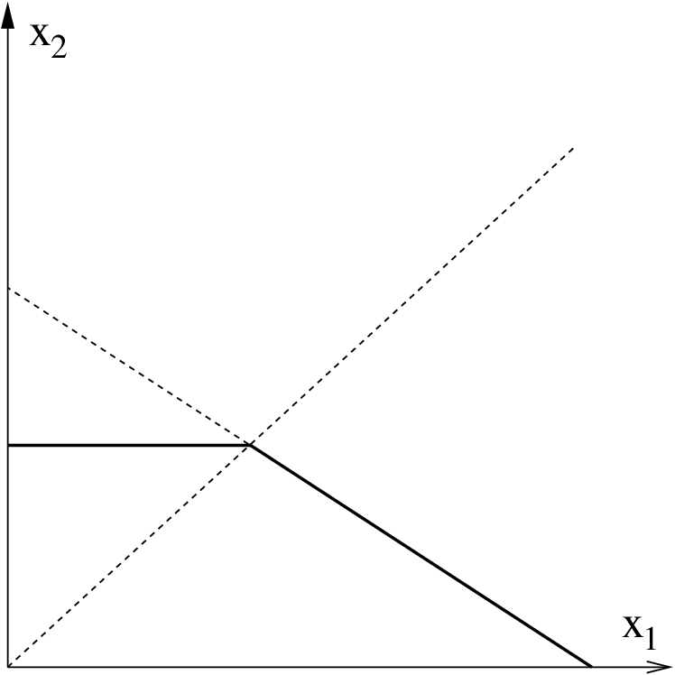
If , one has and
If , one has and
We conclude that the function is non-decreasing for and consequently cannot converge to zero, thus a contradiction.
The Jacobian matrix of dynamics (3) at the non-trivial equilibrium is of the following form in coordinates
Recall that is Hurwitz. One has
The function being concave, one has
. Along with the inequalities and , one deduces .
Recall from Corollary 2 that one has
.
Then the inequality is
necessarily satisfied. Finally, we have shown and , that guarantee the
exponential stability of the non-trivial equilibrium
.
Remark. The wash-out equilibrium is not necessarily hyperbolic. This explains why we cannot use the Convergence Theorem for asymptotically autonomous dynamics given in Appendix F of [29].
References
- [1] de Gooijer C.D., W.A.M. Bakker, H.H. Beeftink and J. Tramper (1996), Bioreactors in series: an overview of design procedures and practical applications, Enzyme and Microbial Technology, Vol. 18, pp. 202–219.
- [2] de Gooijer C.D., Beeftink H.H. and Tramper J. (1996) Optimal design of a series of continuous stirred tank reactors containing immobilised growing cells. Biotechnology Letters., Vol. 18, pp. 397–402.
- [3] Doran P. (1999) Design of mixing systems for plant cell suspensions in stirred reactors. Biotechnology Progress, Vol. 15, pp. 319–335.
- [4] A.K. Dramé, Harmand J., Rapaport, A. and Lobry, C. Multiple steady state profiles in interconnected biological systems. Mathematical and Computer Modelling of Dynamical Systems, Vol. 12, No. 5, pp. 379-3-9, 2006.
- [5] A.K. Dramé, Lobry, C., Harmand, J., Rapaport, A. and Mazenc, F. Multiple stable equilibrium profiles in tubular bioreactors. Mathematical and Computer Modelling. 48 (11-12), pp. 1840–1853, 2008.
- [6] Grobicki A. and Stuckey D.C. (1992) Hydrodynamic characteristics of the anaerobic baffled reactor. Water Research. Vol. 26, pp. 371–378.
- [7] Grady L. G. Daigger and H. Lim (1999) Biological Wastewater Treatment, 3nd Edition, Environmental Science and Pollution Control Series. Ed. Marcel Dekker, New-York.
- [8] Gravel D., F. Guichard, M. Loreau and N. Mouquet (2010). Source and sink dynamics in metaecosystems. Ecology, Vol. 91, pp. 2172–2184.
- [9] Hanski I. Metapopulation ecology. Oxford University Press, 1999.
- [10] Harmand J., A. Rapaport and A. Trofino (2003), Optimal design of two interconnected bioreactors–some new results, American Institute of Chemical Engineering Journal, Vol. 49, No. 6, pp. 1433–1450.
- [11] Harmand J., A. Rapaport and A. Dramé (2004), Optimal design of two interconnected enzymatic reactors, Journal of Process Control, Vol. 14, No. 7, pp. 785–794.
- [12] Harmand J. and D. Dochain (2005), Towards a unified approach for the design of interconnected catalytic and auto-catalytic reactors, Computers and Chemical Engineering, Vol. 30, pp. 70–82.
- [13] Hill G.A. and C.W. Robinson (1989), Minimum tank volumes for CFST bioreactors in series, The Canadian Journal of Chemical Engineering, Vol. 67, pp. 818–824.
- [14] Hu W.-S., K. Wlashchin, M. Betenbaugh, F. Wurm, G. Seth and W. Zhou (2007) Cellular Bioprocess Technology, Fundamentals and Frontier. Lectures Notes. University of Minesota.
- [15] Levenspiel O. (1999) Chemical reaction engineering. 3nd edn. Wiley, New York.
- [16] Lovitt, R. and Wimpenny, J. The gradostat: a bidirectional compound chemostat and its applications in microbial research. Journal of General Microbiology, Vol. 127, pp. 261–268, 1981.
- [17] Luyben K. and Tramper J. (1982), Optimal design for continuously stirred tank reactors in series using Michaelis-Menten kinetics, Biotechnology and Bioengineering, Vol. 24, pp. 1217–1220.
- [18] MacArthur, R. H. and Wilson, E. The Theory of Island Biogeography. Princeton University Press, 1967.
- [19] Mischaikow M., H. Smith and H. Thieme (1995), Asymptotically autonomous semiflows: chain recurrence and Lyapunov functions, Transactions of the American Mathematical Society, Vol. 347, No. 5, pp. 1669–1685.
- [20] Monod, J. La technique de la culture continue: théorie et applications. Annales de l’Institut Pasteur, Vol. 79, pp. 390–410, 1950.
- [21] Nakaoka S. and Y. Takeuchi (2006) Competition in chemostat-type equations with two habitats. Mathematical Biosciences, Vol. 201, pp. 157–171.
- [22] Nelson M. I. and H.S. Sidhu (2006) Evaluating the performance of a cascade of two bioreactors, Chemical Engineering Science, Vol. 61, pp. 3159–3166.
- [23] Novick, A., and L. Szilard Description of the chemostat. Science, Vol. 112, pp. 715–716, 1950.
- [24] Rapaport A.,Harmand J. and Mazenc F. (2008) Coexistence in the design of a series of two chemostats. Nonlinear Analysis, Real World Applications Vol. 9, pp. 1052–1067.
- [25] Roca E., C. Ghommidh, J. M. Navarro and J. M. Lema (1995) Hydraulic model of a gas-lift bioreactor with flocculating yeast. Bioprocess and Biosystems Engineering, Vol. 12, No. 5, pp. 269–272.
- [26] Roux G., B. Dahhou and I. Queinnec (1994) Adaptive non-linear control of a continuous stirred tank bioreactor. Journal of Process Control, Vol. 4, No. 3, pp. 121–126.
- [27] A. Saddoud, T. Sari, A. Rapaport, R. Lortie, J. Harmand and E. Dubreucq (2010), A mathematical study of an enzymatic hydrolysis of a cellulosic substrate in non homogeneous reactors. Proceedings of the IFAC Computer Applications in Biotechnology Conference (CAB 2010), Leuven, Belgium, July 7–9..
- [28] Scheel, A. and Van Vleck, E. Lattice differential equations embedded into reaction-diffusion systems. Proceedings of the Royal Society Edinburgh Section A 139 (1), pp. 193–207, 2009.
- [29] Smith H. and P. Waltman (1995) The theory of chemostat, dynamics of microbial competition, Cambridge Studies in Mathematical Biology, Cambridge University Press.
- [30] Stephanopoulos G. and A. G. Fredrickson (1979), Effect of inhomogeneities on the coexistence of competing microbial populations, Biotechnology and Bioengineering, Vol. 21, pp. 1491–1498.
- [31] Valdes-Parada F., J. Alvarez-Ramirez and A. Ochoa-Tapia (2005) An approximate solution for a transient two-phase stirred tank bioreactor with nonlinear kinetics. Biotechnology progress. Vol. 21, No. 5, pp. 1420–1428 .
- [32] Van’t Riet, K. and J. Tramper (1991) Basic bioreactor design. Marcel Dekker, New-York.