Twisted Hubbard Model for Sr₂IrO₄: Magnetism and Possible High Temperature Superconductivity.

Various Ir oxides have recently become the platform to study the interplay between strong spin-orbit(SO) interaction and strong correlation effects. There has been an experimental observation of a three-dimensional spin liquid in a hyper-kagome structure of Na₄Ir₃O₈[1]. Theoretical proposals such as the realization of correlated topological insulators[2], the Kitaev model[3], and a Dirac semimetal with surface “Fermi arcs”[4] in iridates have been made as well. Here we propose that doped Sr₂IrO₄ may realize high-temperature superconductivity similar to the cuprates.

The crystal structure of Sr₂IrO₄ consists of two-dimensional(2D) IrO₂ layers, similar to the parent compound La₂CuO₄ of the cuprates. The main difference is that the oxygen octahedra surrounding Ir rotate along $c$-axis by about $11^{\circ}$ in a staggered pattern, enlarging the unit cell by $\sqrt{2}\times\sqrt{2}\times 2$ [5]. The electronic structure of Sr₂IrO₄ is quasi-2D, but is expected to have several differences from the cuprates. Ir⁴⁺ has the electronic structure $5d^{5}$, so the $t_{2g}$ levels should to be active, while Cu²⁺ with $3d^{9}$ configuration has only the top $e_{g}$ level active. Ir as a $5d$ transition metal is expected to have weaker correlation effects than $3d$ elements(e.g. Cu). At this point one may expect that Sr₂IrO₄ is a (multi-band) weakly correlated metal. But strong spin-orbit coupling of Ir dramatically changes the story. The $t_{2g}$ levels are split by SO interactions into a higher energy Kramers doublet (the pseudospin-1/2 or $J_{\rm eff}=1/2$ states) and two pairs of lower energy ones[6]. These $J_{\rm eff}=1/2$ states are equal weight superpositions of all three $t_{2g}$ orbitals, and this has been confirmed experimentally by resonant x-ray scattering[7] and theoretically by LDA+SO+U calculation[8]. With $d^{5}$ configuration of Ir the $J_{\rm eff}=1/2$ states are half-filled. They have much smaller band width than expected for the $t_{2g}$ levels without SO interaction and therefore have effectively enhanced correlation effect. In the end Sr₂IrO₄ is a Mott insulator and exhibits magnetic order below 240K[9, 10, 11].

It is then tempting to make the analogy between Sr₂IrO₄ and the cuprates and speculate that doped Sr₂IrO₄ can also realize the interesting physics in doped cuprates, e.g. superconductivity, pseudogap, stripe formation, etc.. But strong SO interaction, different active orbitals and the rotation of oxygen octahedra seem to significantly complicate the problem. For example, Sr₂IrO₄ has very anisotropic susceptibility and shows ferromagnetism(FM) with large ferromagnetic moment $\sim 0.14\mu_{B}$ per Ir[12], which was attributed to Dzyaloshinskii-Moriya(DM) interaction generated by the rotation of oxygen octahedra. However it has been pointed out by Jackeli and Khaliullin[3] that the DM interaction can be removed by staggered rotation of pseudospin space on Ir sites. We will extend this consideration to the electronic model in a slightly different perspective and discuss more details and consequences of this mapping. Finally we will argue that the analogy between Sr₂IrO₄ and the cuprates can be established with careful interpretation, and that interesting physics of doped cuprates may also be realized in doped Sr₂IrO₄.

The mapping to one band Hubbard model.

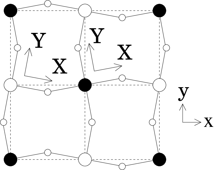
To begin with we will treat Sr₂IrO₄ as quasi-2D and consider only one IrO₂ layer, which is schematically illustrated in Fig. 1. Label the rotation angle of oxygen octahedron around Ir site $j$ by $\theta_{j}=\epsilon_{j}\theta$, with $\epsilon_{j}=\pm 1$ for the two sublattices and $\theta\approx 11^{\circ}$ from experiments[5]. The crystal-field splitting of $t_{2g}$ and $e_{g}$ levels and projection to $J_{\rm eff}=1/2$ states should be implemented in the rotated local cubic axis. Label the global axis by $x,y,z$ and local cubic axis (on site $j$) by $X,Y,Z$ (see Fig. 1). The unit vectors of these two coordinates systems are related by

The $J_{\rm eff}=1/2$ states are (see e.g. Ref. [6], the phase convention here is slightly different, $\mathbbm{i}=\sqrt{-1}$)

$XZ,YZ,XY$ are the $t_{2g}$ orbitals defined in the local cubic axis. $\uparrow,\downarrow$ indicate spin states (defined also in the local cubic axis). Note that although the elongation of oxygen octahedra along $c$-axis is expected to change the relative weights of the three orbitals[6, 3], this has not been observed in resonant x-ray scattering experiment[7] or LDA+SO+U calculation[8].

As the first approximation, the effective electronic Hamiltonian should be the projection of full Hamiltonian on the subspace of $J_{\rm eff}=1/2$ states. Considering first the Hamiltonian on the $t_{2g}$ subspace, we expect the following, 1) the $t_{2g}$ orbitals should be defined in the local cubic axis basis, because the crystal-field on Ir $5d$ orbitals from neighboring oxygens is diagonal only in the local cubic axis; 2) assuming that hoppings between Ir sites are mediated by the oxygen $2p$ orbitals, simple symmetry consideration shows that effective hoppings between nearest-neighbor Ir are orbital diagonal(one $t_{2g}$ orbital does not hop to another orbital) only in the local cubic axis basis; 3) if the spin spaces are defined in the global axis basis, the effective hoppings of Ir $t_{2g}$ orbitals will be real. Two tight-binding models on the $t_{2g}$ subspace have been obtained by fitting LDA+SO+U dispersions in Ref. [8] and Ref. [13], and both have this property of real orbital diagonal hoppings, but no clear interpretation was given. The discussion above shows that the orbitals in these models should be interpreted as the $t_{2g}$ orbitals in the local cubic axis, while the spins in these models are defined in the global axis.

The spin space on every site should be first rotated to local axis before the projection to the $J_{\rm eff}=1/2$ states, because the spins used in (2) are defined in local axis. Namely we need to interpret the electron operators $c_{j,a,\nu}^{\dagger}$ used in these models, on site $j$ for orbital $a=XZ,YZ,XY$ with spin $\nu$, as creation operators for the states $e^{\mathbbm{i}\epsilon_{\nu}\theta_{j}/2}|j,a,\nu\rangle$, where $\epsilon_{\nu}=\pm 1$ for spin index $\nu=\uparrow,\downarrow$ respectively.

Define $d_{\uparrow}$ and $d_{\downarrow}$ as the annihilation operators for the $|J_{\rm eff}^{z}=\pm 1/2\rangle$ states (2) respectively. The projection on the $J_{\rm eff}=1/2$ subspace is implemented by the following substitution, $c_{j,XY,\nu}^{\dagger}\to-\epsilon_{\nu}\mathbbm{i}\sqrt{1/3}\,e^{\mathbbm{i}\epsilon_{\nu}\theta_{j}/2}d_{j,\nu}^{\dagger}$, $c_{j,XZ,\nu}^{\dagger}\to\epsilon_{\nu}\sqrt{1/3}\,e^{\mathbbm{i}\epsilon_{\nu}\theta_{j}/2}d_{j,-\nu}^{\dagger}$, and $c_{j,YZ,\nu}^{\dagger}\to-\mathbbm{i}\sqrt{1/3}\,e^{\mathbbm{i}\epsilon_{\nu}\theta_{j}/2}d_{j,-\nu}^{\dagger}$. The onsite interactions between $t_{2g}$ orbitals will be projected into an onsite $U$ term of the Hubbard model for the $J_{\rm eff}=1/2$ states due to time-reversal symmetry and charge conservation.

We take as a concrete example the tight-binding model of Ref. [13]. It involves nearest-neighbor(NN) $XY$ hopping $t_{1}=0.36$eV, NN $XZ$($YZ$) hopping along $x$($y$) direction $t_{4}=0.37$eV, NN $XZ$($YZ$) hopping along $y$($x$) direction $t_{5}=0.06$eV, next-nearest-neighbor $XY$ hopping $t_{2}=0.18$eV, and third-neighbor $XY$ hopping $t_{3}=0.09$eV. The resulting one band Hubbard model after projection is

with $\alpha=\uparrow,\downarrow$, and the effective hoppings are $t=(1/3)(t_{1}+t_{4}+t_{5})\cos\theta\approx 0.258{\rm eV}$, $\bar{t}=(1/3)(t_{1}-t_{4}-t_{5})\sin\theta\approx-0.0045{\rm eV}$, $t^{\prime}=(1/3)t_{2}\approx 0.06{\rm eV}$, $t^{\prime\prime}=(1/3)t_{3}\approx 0.03{\rm eV}$. $\bar{t}$ is very small and will be ignored hereafter. In general $\bar{t}$ can be absorbed into $t$ by a unitary transformation $d_{j,\alpha}\to e^{\mathbbm{i}\epsilon_{\alpha}\epsilon_{j}\phi/2}\tilde{d}_{j,\alpha}$ with $\phi={\rm arc}\tan(\bar{t}/t)$, but we will not elaborate on this. The value of $U$ has been estimated as $\sim 2{\rm eV}$[8, 11]. This $t-t^{\prime}-t^{\prime\prime}-U$ model has been widely used as an effective model for the cuprates, although the parameters here have different values.

With large $U$ and at half-filling the model (3) is an Mott insulator described by a pseudospin-1/2 model with SU(2) symmetry. If second- and third-neighbor $t^{\prime},t^{\prime\prime}$ are ignored the half-filling pseudospin model to the lowest order of $t/U$ is just the Heisenberg AFM model of pseudospins $\mathbf{J}$, $H_{AFM}=\sum_{<jk>}(4t^{2}/U)\mathbf{J}_{j}\cdot\mathbf{J}_{k}$. Each pseudospin has three components ($a=1,2,3$) $J_{j,a}=(1/2)\sum_{\alpha,\beta}d_{j,\alpha}^{\dagger}(\sigma^{a})_{\alpha\beta}^{\vphantom{\dagger}}d_{j,\beta}^{\vphantom{\dagger}}$, where $\sigma$ are Pauli matrices and $\alpha,\beta=\uparrow,\downarrow$ label the $J_{\rm eff}^{z}=\pm 1/2$ states.

Coupling to external magnetic field. Although the effective model (3) looks exactly like the model of the cuprates, the coupling to external magnetic field in Sr₂IrO₄ is quite different.

Assume the coupling of magnetic field $\mathbf{B}$ on Ir $5d$ orbitals is described by the atomic form (more careful treatment can be found in, e.g., Ref. [6]), $H_{B}=-\mu_{B}\mathbf{B}\cdot(\mathbf{L}+2\mathbf{S})$, where $\mu_{B}$ is the Bohr magneton. After projection to the $J_{\rm eff}=1/2$ states it becomes $H_{B}=2\mu_{B}\mathbf{B}\cdot\mathbf{J}=2\mu_{B}(B_{X}J_{1}+B_{Y}J_{2}+B_{Z}J_{3})$. Note that $B_{X,Y,Z}$ are components of field on the local cubic axis, $B_{X}=\mathbf{B}\cdot\hat{X}$ etc.. Use the relation (1), the coupling on site $j$ in terms of the field components on the global axis, $B_{x},B_{y},B_{z}$, is

Therefore the observable magnetic moment $\mathbf{M}_{j}$ on site $j$ has the following components on the global axis,

If $\bar{t}$ in (3) is not ignored $\theta\approx 11^{\circ}$ in (5) should be replaced by $\theta-{\rm arc}\tan(\bar{t}/t)\approx 12^{\circ}$. This nontrivial relation between moments $\mathbf{M}$ and pseudospins $\mathbf{J}$, namely a $g$-tensor with a staggered antisymmetric component, has several interesting consequences which we list below.

• •

  By quantum Monte Carlo studies[14] the square lattice Heisenberg model has a Néel ground state with staggered “magnetization” $|\langle\epsilon_{j}\mathbf{J}_{j}\rangle|\approx 0.307$. However because of the relation (5), the ordered moments do not form a simple collinear Néel pattern. If the ordered moments lie in the $xy$ plane, they will be rotated together with the oxygen octahedra in a staggered pattern therefore create a net ferromagnetic moment per site, $2\mu_{B}\cdot|\langle\epsilon_{j}\mathbf{J}_{j}\rangle|\cdot\sin\theta\approx 0.12\mu_{B}$. This is very close to the experimentally observed value $0.14\mu_{B}$ [12].

• •

  By the relation (5) we can relate pseudospin correlation functions of model (3) to moment correlation functions which is actually measured by susceptibility or magnetic neutron/x-ray scattering experiments. The Fourier components of moments with wavevector $\mathbf{q}$ and frequency $\omega$ is related to pseudospins by,

  $$\begin{split}&M_{\mathbf{q},\omega,x}=-2\mu_{B}[\cos\theta\,J_{\mathbf{q},\omega,1}-\sin\theta\,J_{\mathbf{q}+\mathbf{Q},\omega,2}],\\ &M_{\mathbf{q},\omega,y}=-2\mu_{B}[\cos\theta\,J_{\mathbf{q},\omega,2}+\sin\theta\,J_{\mathbf{q}+\mathbf{Q},\omega,1}],\\ &M_{\mathbf{q},\omega,z}=-2\mu_{B}\,J_{\mathbf{q},\omega,3}.\end{split}$$

  where $\mathbf{Q}=(\pi,\pi)$ is the wavevector of Néel order. In the paramagnetic phase the dynamical susceptibility $\chi^{ab}(\mathbf{q},\omega)$, which is proportional to the “moment structure factor” $\langle M_{\mathbf{q},\omega,a}M_{-\mathbf{q},-\omega,b}\rangle$, is related to the dynamical pseudospin susceptibility $\chi^{ab}_{J}(\mathbf{q},\omega)=\delta_{ab}\chi_{J}(\mathbf{q},\omega)\propto\langle\mathbf{J}_{\mathbf{q},\omega}\cdot\mathbf{J}_{-\mathbf{q},-\omega}\rangle$ by

  $$\begin{split}&\chi^{xx}(\mathbf{q},\omega)=\chi^{yy}(\mathbf{q},\omega)\\ =\ &\cos^{2}\theta\,\chi_{J}(\mathbf{q},\omega)+\sin^{2}\theta\,\chi_{J}(\mathbf{q}+\mathbf{Q},\omega),\end{split}$$

  $\chi^{zz}(\mathbf{q},\omega)=\chi_{J}(\mathbf{q},\omega)$, and other components of $\chi^{ab}$ are zero. In particular the measured static uniform ($\omega=0,\mathbf{q}=0$) susceptibility in $xy$ plane is actually a mixture of the uniform and staggered susceptibility of the SU(2) invariant Hubbard/Heisenberg model. This explains in a different perspective the measured large anisotropy of uniform susceptibility and the ferromagnetic Curie-Weiss law [12]. In our picture the anisotropy is not mainly from easy axis interaction suggested by Ref. [12] but from the mixing of large staggered susceptibility, and the FM Curie-Weiss law comes from the contribution of staggered susceptibility close to AFM Nèel order of pseudospins.

• •

  In the high temperature paramagnetic phase above the Néel ordering temperature, the measured moment-moment correlation will be dominated by the staggered pseudospin correlation of a SU(2) invariant model, although the measured susceptibility shows significant anisotropy. The moment-moment correlation length will behave like the 2D Heisenberg model[15], which has recently been observed by magnetic x-ray scattering [16].

Possible high-temperature superconductivity. If the one band Hubbard model (3) is indeed a good approximation of the electronic struture of Sr₂IrO₄, and if the high-temperature superconductivity in doped cuprates is indeed described by the one band Hubbard model, a natural consequence is that doped Sr₂IrO₄ will realize high-temperature superconductivity. In the following we list several direct consequences from this analogy.

• •

  It is believed that the sign and magnitude of $t^{\prime}$ is important for high-Tc in the cuprates and likely responsible for the particle-hole asymmetry of the phase diagram. (see e.g., Ref. [17]). The relative magnitude $|t^{\prime}/t|\approx 0.23$ for Sr₂IrO₄ is similar to the cuprates. However the sign of $t^{\prime}$ for Sr₂IrO₄ is opposite to that of the cuprates. This can be remedied by a particle-hole transformation $d_{j,\alpha}^{\vphantom{\dagger}}\to\epsilon_{j}^{\vphantom{\dagger}}d_{j,\alpha}^{\dagger}$. Therefore we expect that the doping phase diagram of Sr₂IrO₄ will be the particle-hole conjugate of the cuprates, in particular high-Tc will be easier to achieve on the electron-doped side of Sr₂IrO₄, e.g. with La substitution of Sr. Interestingly electron-doped Sr₂IrO_4-δ has recently been synthesized and metallic behavior was reported for $\delta=0.04$ [18].

• •

  The interlayer hopping of the cuprates is of the form $t_{\perp}(k_{\parallel})=t_{\perp 0}\,v^{2}$ with $v=(\cos k_{x}-\cos k_{y})/2$, due to the $d_{x^{2}-y^{2}}$ orbital content[19]. This together with the $d_{x^{2}-y^{2}}$ nodal pairing symmetry significantly suppress transport along $c$-axis, making the superconducting properties of the cuprates very anisotropic. However the resistivity anisotropy $\rho_{c}/\rho_{ab}$ of Sr₂IrO₄ is only $10^{2}-10^{3}$ [20], very small compared to $10^{4}-10^{5}$ of the cuprates[21], which implies a larger $t_{\perp 0}$ for Sr₂IrO₄. The active orbitals for Sr₂IrO₄ is very different from the cuprates and the factor $v^{2}$ should be different and not vanish on the nodal direction. Both facts suggest that Sr₂IrO₄ should have more isotropic superconducting properties which is beneficial for practical applications.

• •

  The pairing will be a pseudospin singlet $d_{x^{2}-y^{2}}$ pairing and in many ways behave like the d-wave pairing of the cuprates. Phase sensitive and other indirect measurements used to determine the d-wave symmetry in the cuprates can be applied to doped Sr₂IrO₄ as well.

• •

  The energy scale of the one band Hubbard model for Sr₂IrO₄ is lower than that of the cuprates by about $50\%$. Therefore the $T_{c}$ of doped Sr₂IrO₄ will likely be lower than the cuprates.

Discussion and Conclusion. The one band Hubbard model (3) is of course the zeroth order approximation of the low energy electronic structure of Sr₂IrO₄. In real material the mixing between the $J_{\rm eff}=1/2$ states and other states will generate anisotropy in pseudospin interactions, which will be important close to and below the Néel temperature. For magnetic properties above the Néel temperature and for electron-doped Sr₂IrO₄ we believe this one band Hubbard model is still a good description.

The projection to one band Hubbard model was also implemented in Ref. [8]. The resulting hoppings reported in Equ. (7)(8) of Ref. [8] suggest that the authors of Ref. [8] interpreted the orbitals in their $t_{2g}$ tight-binding model as the global axis basis $xz,yz,xy$. Here we have argued that the orbitals should be interpreted as the local axis basis which produces a projection result [$\bar{t}_{0}=-(2t_{0}/3)\cos\theta$ and $\bar{t}_{1}=0$] different from Ref. [8].

In summary we have performed the projection of the electronic structure of Sr₂IrO₄ to the $J_{\rm eff}=1/2$ states and carefully deduced the resulting one band Hubbard model and its interpretation. We provide another perspective on the magnetic properties of Sr₂IrO₄ by viewing it as a SU(2) invariant Hubbard/Heisenberg pseudospin-1/2 model, but with a twisted relation (5) between the observable moments and the pseudospin degrees of freedom, namely a $g$-tensor with staggered antisymmetric component. One direct consequence is that the measured uniform susceptibility in $ab$ plane is actually a mixture of uniform and staggered susceptibility of SU(2) invariant Hubbard/Heisenberg model. Despite the complication of strong SO interaction, different active orbitals and structure distortion, the effective one band Hubbard model of Sr₂IrO₄ remarkably resembles the cuprates. We thus propose that doped Sr₂IrO₄ can realize high-temperature superconductivity, and potentially other interesting physics of the cuprates. By comparing the model parameters we suggest that electron-doping of Sr₂IrO₄ will be the analogue of hole-doping of the cuprates. This can be achieved by La substitution of Sr, or O deficiency [18], and maybe by field effect on thin films[22], or interfacing with other oxides[23]. We hope these simple theoretical observations will stimulate more experimental research on Sr₂IrO₄.

Acknowledgment The authors thank Leon Balents, Dung-Hai Lee, Patrick A. Lee, and Michael Norman for helpful discussions. TS was supported by NSF through the grant DMR-1005434.

References

- [1] Y. Okamoto, M. Nohara, H. Aruga-Katori, and H. Takagi, Phys. Rev. Lett. 99, 137207 (2007).
- [2] A. Shitade, H. Katsura, J. Kuneš, X.-L. Qi, S.-C. Zhang, and N. Nagaosa, Phys. Rev. Lett. 102, 256403 (2009); D. A. Pesin, and Leon Balents, Nat. Phys. 6, 376 (2010); Bohm-Jung Yang, and Yong Baek Kim, Phys. Rev. B 82, 085111 (2010).
- [3] G. Jackeli, and G. Khaliullin, Phys. Rev. Lett. 102, 017205 (2009).
- [4] Xiangang Wan, A. M. Turner, A. Vishwanath, and S. Y. Savrasov, arXiv:1007.0016 (2010).
- [5] M. K. Crawford, M. A. Subramanian, R. L. Harlow, J. A. Fernandez-Baca, Z. R. Wang, and D. C. Johnston, Phys. Rev. B 49, 9198 (1994); Q. Huang, J. L. Soubeyroux, O. Chmaissem, I. Natali Sora, A. Santoro, R. J. Cava, J. J. Krajewski, and W. F. Peck, Jr., J. Sol. St. Chem. 112, 355 (1994).
- [6] B. Bleaney, and M. C. M. O’Brien, Proc. Phys. Soc. B 69, 1216 (1956).
- [7] B. J. Kim, H. Ohsumi, T. Komesu, S. Sakai, T. Morita, H. Takagi, T. Arima, Science 323, 1329 (2009).
- [8] H. Jin, H. Jeong, T. Ozaki, and J. Yu, Phys. Rev. B 80, 075112 (2009).
- [9] R. J. Cava, B. Batlogg, K. Kiyono, H. Takagi, J. J. Krajewski, W. F. Peck, Jr., L. W. Rupp, Jr., and C. H. Chen, Phys. Rev. B 49, 11890 (1994).
- [10] S. J. Moon, M. W. Kim, K. W. Kim, Y. S. Lee, J.-Y. Kim, J.-H. Park, B. J. Kim, S.-J. Oh, S. Nakatsuji, Y. Maeno, I. Nagai, S. I. Ikeda, G. Cao, and T. W. Noh, Phys. Rev. B 74, 113104 (2006).
- [11] B. J. Kim, Hosub Jin, S. J. Moon, J.-Y. Kim, B.-G. Park, C. S. Leem, Jaejun Yu, T.W. Noh, C. Kim, S.-J. Oh, J.-H. Park, V. Durairaj, G. Cao, and E. Rotenberg, Phys. Rev. Lett. 101, 076402 (2008).
- [12] G. Cao, J. Bolivar, S. McCall, J. E. Crow, and R. P. Guertin, Phys. Rev. B 57, 11039(R) (1998).
- [13] H. Watanabe, T. Shirakawa, and S. Yunoki, to appear in Phys. Rev. Lett. (2010).
- [14] J. D. Reger, and A. P. Young, Phys. Rev. B 37, 5978 (1988); A. W. Sandvik, Phys. Rev. B 56, 11678 (1997).
- [15] S. Chakravarty, B.I. Halperin, D.R. Nelson, Phys. Rev. B 39, 2344 (1989); M.S. Makivić, H.-Q. Ding, Phys. Rev. B 43, 3562 (1991).
- [16] Shigeki Fujiyama, presentation in the “Highly Frustrated Magnetism 2010” conference, August 2010 (unpublished).
- [17] P. A. Lee, N. Nagaosa, and X.-G. Wen, Rev. Mod. Phys. 78, 17 (2006).
- [18] O.B. Korneta, Tongfei Qi, S. Chikara, S. Parkin, L. E. De Long, P. Schlottmann, and G. Cao, Phys. Rev. B 82, 115117 (2010).
- [19] O. K. Anderson, A. I. Liechtenstein, O. Jepsen, and F. Paulsen, J. Phys. Chem. Solids 56, 1573 (1995).
- [20] S. Chikara, O. Korneta, W. P. Crummett, L. E. DeLong, P. Schlottmann, and G. Cao, Phys. Rev. B 80, 140407(R) (2009).
- [21] S. Martin, A. T. Fiory, R. M. Fleming, L. F. Schneemeyer, and J. V. Waszczak, Phys. Rev. B 41, 846 (1990).
- [22] J. T. Ye, S. Inoue, K. Kobayashi, Y. Kasahara, H. T. Yuan, H. Shimotani, and Y. Iwasa, Nat. Mat. 9, 125 (2010).
- [23] J. Mannhart, and D. G. Schlom, Science 327, 1607 (2010).