Torqued fireballs in relativistic heavy-ion collisions
Abstract
We show that the fluctuations in the wounded-nucleon model of the initial stage of relativistic heavy-ion collisions, together with the natural assumption that the forward (backward) moving wounded nucleons emit particles preferably in the forward (backward) direction, lead to an event-by-event torqued fireball. The principal axes associated with the transverse shape are rotated in the forward region in the opposite direction than in the backward region. On the average, the standard deviation of the relative torque angle between the forward and backward rapidity regions is about for the central and for the mid-peripheral collisions. The hydrodynamic expansion of a torqued fireball leads to a torqued collective flow, yielding, in turn, torqued principal axes of the transverse-momentum distributions at different rapidities. We propose experimental measures, based on cumulants involving particles in different rapidity regions, which should allow for a quantitative determination of the effect from the data. To estimate the non-flow contributions from resonance decays we run Monte Carlo simulations with THERMINATOR. If the event-by-event torque effect is found in the data, it will support the assumptions concerning the fluctuations in the early stage of the fireball formation, as well as the hypothesis of the asymmetric rapidity shape of the emission functions of the moving sources in the nucleus-nucleus collisions.
Keywords:
relativistic heavy-ion collisions, RHIC, LHC, forward-backward correlations, wounded nucleonspacs
25.75.-q, 25.75Gz, 25.75.LdI Introduction
It is believed that the forward-backward (FB) rapidity correlations may reveal important information on the mechanism of particle production in high-energy hadronic and nuclear collisions. Long-range rapidity correlations uncover properties of the dynamical system at a very early stage. For that reason the FB multiplicity correlations have been studied experimentally [1, *Alpgard:1983xp, *Aivazian:1988ui, *Steinberg:2005ec, *Tarnowsky:2006nh, *Srivastava:2007ei, *:2009qa, *:2009dqa, 9] and theoretically [10, *Capella:1982ru, *Fialkowski:1982kt, *DiasdeDeus:1987bn, *Shuryak:2000pd, *Brogueira:2006yk, *Brogueira:2007ub, *Haussler:2006rg, *Cunqueiro:2006xe, *Armesto:2006bv, *Koch:2008ia, *Konchakovski:2008cf, *Gelis:2009tg, *Dusling:2009ni, *Brogueira:2009nj, 25, 26, *Fialkowski:2004wh, *Brodsky:1977de, *Adil:2005qn, *Adil:2005bb, 31, *Bzdak:2009xq, *Bialas:2010zb, 34, 35]. In this paper we show that the wounded-nucleon approach [36, 37] to the initial stage of the collisions leads to a new manifestation of the FB fluctuations: the torqued fireball. Specifically, parts of the fireball are rotated in the transverse plane in one direction in the forward rapidity region, and in the opposite direction in the backward rapidity region. The magnitude and sign of the torque angle fluctuate from event to event.
The following ingredients are responsible for the appearance of the torque effect:
- 1.
statistical fluctuations of the transverse density of the sources (wounded nucleons) [38, *Manly:2005zy, *Andrade:2006yh, *Voloshin:2006gz, *Alver:2006wh, *Drescher:2006ca, *Broniowski:2007ft, *Voloshin:2007pc, *Hama:2009pk, *Andrade:2008fa, *Broniowski:2009fm], and
- 2.
On the average, for the studied Au+Au collisions at the highest energies available at the BNL Relativistic Heavy Ion Collider (RHIC), the relative torque angle between the principal axes in the forward and backward rapidity regions is about for the central, and for the mid-peripheral collisions. On the other hand, an experimental observation of nonzero torque angles of the expanding fireball could shed light on the mechanism of the formation of dense matter. A finite torque between reaction planes at different rapidities could influence elliptic and directed flow studies using reaction planes determined in different pseudorapidity intervals [49, *Afanasiev:2009wq].
The paper has three parts, referring subsequently to the early wounded-nucleon phase of the collision (Sect. II), the intermediate hydrodynamic stage (Sect. III), and, finally, the statistical hadronization phase (Sect. IV), where hadrons are produced. In Sect. II.1 we introduce the necessary elements of the wounded-nucleon approach, in particular, the asymmetric rapidity-dependent emission functions [25, 26, 31, 34, 35] of the forward and backward moving wounded nucleons. In Sect. II.2 we explain how statistical fluctuations of the density of the forward and backward moving wounded nucleons in the transverse plane lead to the event-by-event torque effect. Simulations are carried out with GLISSANDO [51] in the so-called mixed model [52, 53, *Back:2004dy], incorporating an admixture of binary collisions into the wounded-nucleon model. We introduce quantitative measures of the torque in Sec. II.3. Specifically, we use the difference of the forward and backward angles of the principal axes, as well as three angles, forward, backward, and central, to construct useful statistical quantities. Next, in Sect. III we present the results of running the 3+1 dimensional (perfect fluid) hydrodynamics, as described in [55]. The calculations show that the torque survives the hydrodynamic stage of the evolution. Then, in Sect. IV.1 we pass to discussing the final stage, namely, the statistical hadronization (for a review, see, e.g. [56]). This stage would wash out the torque effect, unless careful experimental measures are used. This is because even at a fixed spatial geometry of the fireball the finiteness of the number of produced particles causes large fluctuations of the event-plane angle, covering up the torque angle. We thus propose to investigate measures based on cumulants [57], introduced in Sect. IV.2. They are constructed in such a way that the relative FB torque angle can be extracted. We examine the non-flow contributions to these measures via simulations in THERMINATOR [58], proving that it is possible to find the torque effect with the proposed methods in the large-statistics RHIC data. In Sect. IV.4 we repeat this analysis for the particles taken from three rapidity bins, forward, backward, and central, with similar conclusions.
II Torqued fireball
In this Section we describe the earliest stage of the relativistic heavy-ion collision in terms of the wounded-nucleon model [36, 37]. All simulations are carried out for the Au+Au collisions at the highest RHIC energy of GeV.
II.1 Wounded nucleons with rapidity profiles
The wounded-nucleon [36, *Bialas:2008zza] approach is commonly used to describe the early stage of the heavy-ion collisions. In the collision process nucleons get wounded, i.e. interact inelastically at least once, as well as binary collisions occur. Roughly speaking, wounded nucleon (participants) are responsible for the soft emission, while binary collisions describe hard processes. Both serve as sources for the formation of the density of energy or entropy in the initial fireball. At RHIC, the mixed model [52], where the total number of the produced particles is given by the combination
| (1) |
describes quite successfully the multiplicity data [53, *Back:2004dy]. The proportionality constant depends on the energy of the collision but not on its centrality. Throughout this work we use , corresponding to collisions at GeV [53, *Back:2004dy].
The concept of sources can be extended to account for the rapidity dependence of the produced particles. The pseudorapidity distribution is given as a sum of contributions from the emission of forward and backward going wounded nucleons. Within such a scheme Białas and Czyż successfully described [25] the distribution of charged particles in pseudorapidity in the deuteron-gold collisions [59]. The independent emission from the forward and backward going nucleons determines specific FB multiplicity correlations [31, 34]. In particular, this hypothesis has been tested successfully in Ref. [34] with the FB multiplicity correlation data from the PHOBOS collaboration [9]. Based on this idea, Ref. [35] postulated that in nucleus-nucleus collisions the emission profile defining the initial density (in the space-time rapidity and the transverse plane coordinates , ) has the form
| (2) | |||||
where is the density of the forward and backward going wounded nucleons at a given point in the transverse plane, is the binary collisions density, while and describe the corresponding wounded-nucleon emission profiles. Finally, is the emission profile for the binary collisions. These functions are chosen appropriately, taking into account the following features: the profile () is peaked in the forward (backward) direction, i.e. the wounded nucleon emits mostly in its own forward hemisphere, with a quite broad distribution, whereas the binary profile is (for the collision of identical nuclei) symmetric.
We remark that the asymmetric wounded-nucleon emission functions in Eq. (2) give a tilt away from the beam axis for the initial fireball (in the plane). The hydrodynamic expansion [35] of such a tilted fireball generates the directed flow and for the first time the experimental observations at GeV [60, *Adams:2005ca, *Abelev:2008jga] could be reproduced.
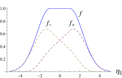
Following Ref. [35], we choose the following parameterizations:
| (3) |
with
The values of parameters, describing the RHIC data after the hydrodynamic evolution [35], are
| (8) |
The profile functions are shown in Fig. 1. We note that by construction . Parametrization (II.1) is chosen in such a way, that after the hydrodynamic evolution and statistical emission [55, 35] one correctly reproduces the spectra [63, *Bearden:2001qq] of particles produced at different rapidities in the Au+Au collisions at the highest RHIC energy.
II.2 Fluctuations and the torque

The initial density of the fireball (2) can be obtained in a Glauber Monte Carlo approach. The densities of the forward and backward going wounded nucleons and of the binary collisions are obtained with Monte Carlo simulations by GLISSANDO [51]. These distributions fluctuate on event-by-event basis. The phenomenon has a purely statistical origin, as the positions on nucleons in nuclei fluctuate. The event-by-event fluctuations in the wounded-nucleon approach are know to cause important effects, such as the increase of the elliptic deformation, resulting in larger elliptic flow [38], or the recently discussed triangular flow [65, *Alver:2010dn, *Petersen:2010cw].
Another effect due to fluctuations, focal to this work, is the event-by-event torque of the fireball. Its appearance is simple to understand. For the sake of simplicity let us consider the situation depicted in Fig. 2. A cluster of wounded nucleons is formed, here drawn at the edge of the fireball. It contains three wounded nucleons moving forward and one moving backward. The cluster causes the twist of the principal axis. However, due to the shape of the emission functions of Fig. 1, the shift is different at various values of the space-time rapidity. At forward there are practically no backward moving wounded nucleons, hence the three forward-moving nucleons cause the torque. In the backward direction only one wounded nucleon from the cluster causes the torque, while in the central region all four nucleons contribute, but according to Eq. (II.1) their relative weight is reduced be a factor of . Thus the relative weight of the effect of the cluster in the forward, backward, and central regions is as . The result is the schematic arrangement of the principal axes as drawn in Fig. 2.
In an actual Monte Carlo simulation many clusters occur and the situation is more complicated, but the origin is as described above. The effect appears on the event-by-event basis and by symmetry the mean value of the torque angle vanishes upon averaging over events. Thus, the effect may only be revealed in event-by-event studies of fluctuations, see Sect. II.3.

A similar phenomenon occurs for the axes of the triangular shape and the axes corresponding to higher Fourier moments in the azimuthal angle. The shape of the fireball is depicted schematically in Fig. 3, where the torque angle, somewhat exaggerated, is shown for the elliptic and triangular deformations. As mentioned above, the torque appears on the event-by-event basis, varying in the direction and value.
II.3 Characteristics of the torqued the fireball
In this subsection we provide quantitative studies of the torque effect at the instant of formation. In a given event, the angle of the principal axis for the Fourier moment of rank- for sources at some is given by the formula
| (9) |
where are the polar coordinates of the source position with respect to the center of mass of the slice of the fireball at some fixed , and is the weight of the source. Explicitly, for the forward-moving wounded nucleons , for the backward ones , while for the binary collisions .11 1 One could also overlay a statistical distribution of weights, as was done in Ref. [51]. All spatial angles are measured relative to the axes perpendicular to the reaction plane. The interpretation of the angle is that the azimuthal Fourier moment of rank is highest along that direction. The angle is defined modulo . For the angle is the angle of the principal axes of the moment of inertia. For brevity of notation, we shall skip the superscript from the rank-2 quantities, while retaining superscripts indicating higher ranks.
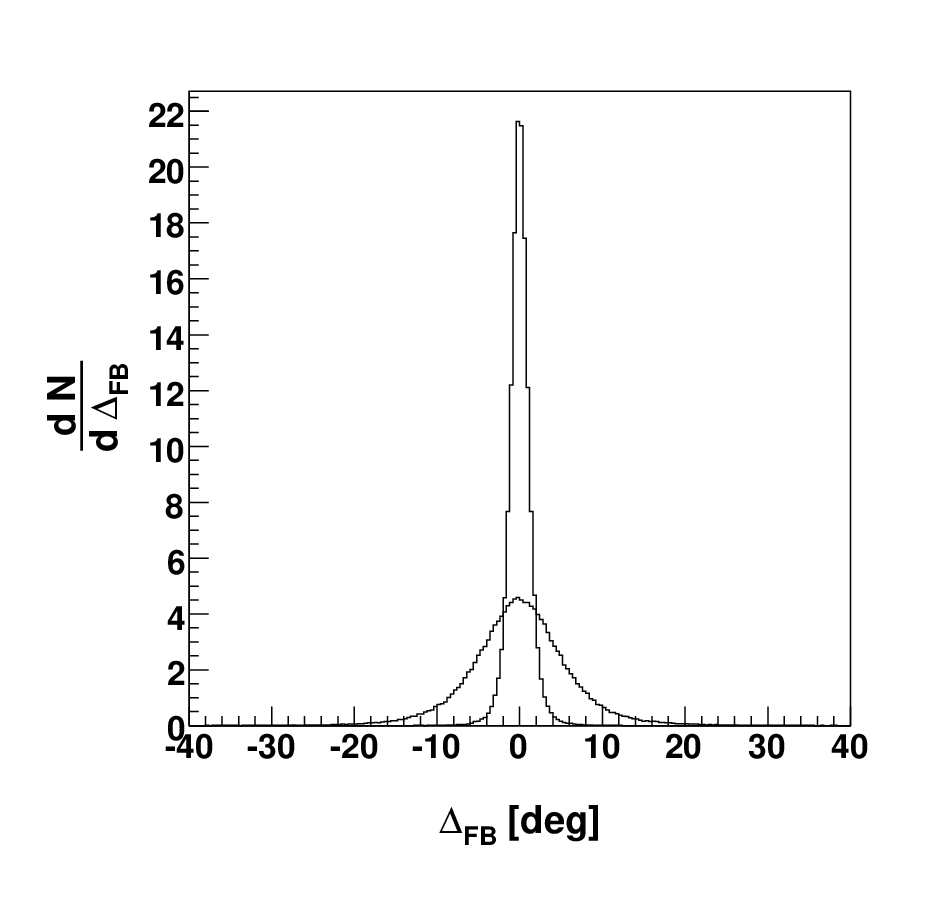
The simplest measure of the torque effect is the difference of the angles at forward and backward values of ,
| (10) |
As argued above, this quantity fluctuates event-by-event. The result of the GLISSANDO simulations is shown in Fig. 4. We plot the event-by-event distribution of for the 20-30% centrality class and (the narrower distribution) and (the wider distribution). According to the previous qualitative discussion illustrated with Fig. 3, the widening of the distribution with increasing is expected. The rms width of the distributions of Fig. 4 for % are for and for . An analogous study for (not shown) yields for and for . Thus the spread enhances with increasing , moreover, the distributions are wider for the central collisions.
For the rank-3 analysis (triangular flow) we have qualitatively the same effect. For % the rms width are for and for , which are larger than for the rank-2 case at the same centrality.


In Figs. 5 and 6 we show the dependence of the rms width of the distributions of and as functions of at various centralities. For the rank-2 case we note that the widths grow gradually from 0 at to at , with the largest angle for the most central events. The rank-3 widths are somewhat larger than in the rank-2 case, except for the most central case. We note that at fixed the dependence on centrality is non-monotonic, with the lowest value for for the rank-2 case and for the rank-3 case. We also note that for the rank-2 case the most central collisions lead to significantly larger torque fluctuations than for the less central collisions, cf. Fig. 5.
One may introduce other measures, involving three angles associated with the forward, backward, and central regions. This might be advantageous, as the central rapidity region is experimentally better covered experimentally. We define the two relative angles
| (11) |
and their covariance,
| (12) |
The forward-backward-central correlation coefficient is defined as
| (13) |
In Fig. 7 we present the 2-dimensional distribution plot of and for the rank-2 case for and the 50-60% centrality class, where the anti-correlation of the angles is clearly visible.22 2 We note that the points in Fig. 7 occupy all quadrants, i.e. there are cases where both shifts and have the same sign. This is because for each rapidity we evaluate independently the center of mass, which is the origin for the transverse coordinate system. If we evaluated the angle in the common system associated with the central rapidity, only the second and fourth quadrants in Fig. 7 would be filled.

Figures 8 and 9 show the rapidity dependence of for the rank-2 and rank-3 cases. We note that these measures drop monotonically with from zero to negative values in the range to , reaching a plateau near . For a fixed the dependence on the centrality class is non-monotonic. From the data of Figs. 8 and 5 one may obtain the correlation of Eq. (13). This quantity grows from the value at up to about at , similarly for the rank-2 and rank-3 cases.


III Hydrodynamics
The intermediate evolution of the dense system formed in relativistic heavy-ion collisions is believed to be governed by hydrodynamics [68, *Kolb:2003dz, *Hama:2005dz, *Huovinen:2006jp, *Hirano:2005xf, *Hirano:2002ds, 74, 55]. The hydrodynamic expansion of the fireball generates a collective velocity field of the hot fluid. The direction of the acceleration of the fluid element is given by pressure gradients. This way the azimuthal eccentricity of the fireball is transformed into the elliptic flow [75], the triangular deformation into the triangular flow [65], and the source tilt into the directed flow of the final hadrons [35]. A similar mechanism generates, on event-by-event basis, a torqued transverse velocity field at different rapidities.
The discussion of the torque of the fireball in the preceding sections concerned the earliest stage of the collision, described within the wounded-nucleon approach. That stage, essentially, prepares the initial condition for the subsequent phases of the evolution. It is necessary to check that the signatures of the torque fluctuations survive these later stages, such that measurable effects can be detected in experiment. Here we investigate the behavior of the rank-2 torque under the hydrodynamic evolution, as the rank-3 case is expected to behave similarly. A rotation of the density in the transverse plane in the torqued fireball scenario, would generate a rotated fluid velocity field. This rotation of the transverse velocity field at each space-time rapidity would lead to a rotation of the reconstructed reaction plane for particles emitted in the corresponding rapidity range.
We apply the 3+1 hydrodynamic evolution of the perfect fluid with a realistic equation of state, implemented for the first time in [76]. This approach is capable of uniformly describing the main experimental features, such as the transverse momentum spectra, , as well as the Hanbury Brown–Twiss correlation radii [74]. Extension to 3+1 dimensions allows to describe also the spectra at non-central rapidities and the directed flow [55, 35].
To demonstrate the effects of the torqued fireball on final particle spectra, we generate the hydrodynamic evolution for the sample value of the impact parameter, fm, which corresponds to the centrality -% [77]. The initial energy density is taken in the form given in Eq. (2), with the wounded nucleon and and binary collision densities calculated in the Glauber model. The details and the parameters of the distribution can be found in [55, 35]. The initial proper time for the evolution is fm/c. To study the torque effect, instead of doing tedious event-by-event hydrodynamic simulations with a whole distribution of torque angles as in Fig. 4, we perform one simulation where the densities of the forward and backward going wounded nucleons are rotated in opposite directions by a fixed angle of which is a value corresponding to the rms width of the distribution of . Thus the initial energy density (2), which is the starting point of our hydrodynamics, becomes
| (14) |
The operator rotates the density of forward going wounded nucleons by the fixed angle, while operator rotates the backward going wounded nucleons in the opposite direction. The density of binary collisions is not rotated, as its emission component is symmetric in .

During the hydrodynamic evolution the direction of the transverse flow is determined by the orientation of the fireball density at a given space-time rapidity. The torque angle of the fluid, , is determined by the requirement that in the frame defined by the principal axes of the transverse flow we have , where are the components of the energy-momentum tensor averaged over the transverse plane. In Fig. 10 we show the evolution of the torque angle of the fluid velocity field in the hydrodynamic calculation. We present the angle as a function of the space-time rapidity after a hydrodynamic evolution lasting , or fm/c. Due to the longitudinal push, the effect decreases somewhat as the evolution time increases, but this quenching is very small. Therefore the torque effect survives the hydrodynamic phase with an almost unchanged magnitude. A sizable twist of the collective velocity field at the freeze-out should give a twist of the distribution of the emitted particles.
We note that the space-time rapidity is not equal to the fluid rapidity, as in a boost-invariant model. Moreover, the transverse momenta and rapidities of final hadrons include a thermal component besides the collective velocity. These effects are addressed in the next section, through the use of a realistic model of statistical hadronization.
IV Hadronization and experimental measures
The final question, of key practical importance for the whole idea, is how to observe the torque of the fireball from the data consisting of momenta of detected particles. In our model approach we adopt the statistical hadronization picture [78], where hadrons (stable and resonances [79], which subsequently decay) are produced at freeze-out according to the Frye-Cooper formalism [80], with a freeze-out temperature of MeV [55, 35]. The difficulty lies in the fact that the finiteness of the number of particles produced in each event causes sizable fluctuations of the principal axes (or the event plane) as determined from the transverse momenta. We denote the relative angle between the event-plane axis and the fireball spatial principal axis as . Despite this difficulty, as we shall see, one can propose measures of even-by-event torque fluctuations that should be possible to be observed in the RHIC data.
Throughout this section denotes the momentum pseudorapidity of produced particles, in distinction of the space-time rapidity of the preceding parts.
IV.1 Fluctuations of principal axes from statistical hadronization

To appreciate the phenomenon of the fluctuation of , let us recall formulas from [44] concerning the fluctuation of the eccentricity and the principal axes due to the finite number of (independent) particles. The angle (dependent on the rank ) is defined in each event as
| (15) |
where all angles are measured with respect to the angle of the principal axis of the fireball, , at a selected window. From Appendix C of Ref. [44], which derives the results based on the central limit theorem, we find that (at a fixed multiplicity ) the event-by-event distribution of is given by
| (16) |
where the short-hand notation is
| (17) |
This distribution is a function of the product and , therefore we expect universality with respect to the rank , as well as scaling with . Both larger multiplicity and larger reduce the fluctuations of the angle .
In Fig. 11 we plot the distribution for the typical value of the flow coefficient for the elliptic flow () with for three values of the multiplicity . We note a large width of the distributions, of the order of for , or even more as or decrease. This spread will have the tendency of washing out the smaller torque angle, unless a suitable method, sensitive to differences of angles in the same pseudorapidity bin, is used.
IV.2 Cumulants
To achieve the goal of observing the torque, similarly to analyses of flow [57, 81], we consider cumulants. In the simplest case of the two-particle cumulant we may take
with denoting the Fourier rank and () being the azimuthal angles of particles emitted in the forward (backward) windows in a selected centrality class. The quantities and are the corresponding multiplicities. The measure is averaged over events, with the number of events in the sample equal to .
When no correlations between particles are present, the distribution function of particles is the product of one-body distributions. The one-body distribution can then be written in the form
| (19) |
Then
| (20) |
where indicates the averaging over events. Non-flow contributions modify the right-hand side at the level , where is the effective multiplicity of particles in the event. These effects, hard to estimate, include resonance decays, conservation laws, Bose-Einstein correlations of identical particles, short-range correlations, etc. The influence of resonance decays will be analyzed via simulations below.
Since we are interested in measuring the average , we need to divide Eq. (20) by . We can do it, for instance, by evaluating the ratio of cumulants, defined as
| (21) | |||||
One may also use higher-order cumulants to generate measures of the torque. For example, the ratio of four-particle cumulants, yields
| (22) | |||||
The practical issue in this kind of studies is the influence of the non-flow contributions on the result.
IV.3 THERMINATOR simulations
The precise estimate of the non-flow effects in the formulas of the previous section is not easy. To obtain a realistic estimate of the influence of resonance decays, we have run THERMINATOR [58], generating 100000 events (in one centrality class) from a fireball with a torqued hypersurface, resulting from running the 3+1 perfect hydrodynamics [35] on the torqued initial condition, as described in Sect. III. In Figs. 12 we present the results for centrality , where, at freeze-out, the torque angles in the forward and backward directions differ by , as in Fig. 10.
First, we check if THERMINATOR is capable of reproducing the (fixed) input torque angle. For this purpose we take into account primordial particles (those created at the freeze-out hypersurface) only, thus disregarding resonance decays. The result, shown in Fig. 12 with squares, shows a nice agreement between the cumulant measures (21,22) and the functions and , shown with lines, evaluated directly from the fireball torque angle shown in Fig. 10 (we take here the case of the evolution time equal of 6 fm/c). For comparison, the triangles indicate the result of the calculation without the torque, . The agreement shows that without the non-flow contribution from resonance decays the accumulated statistics of 100000 THERMINATOR events per centrality class is sufficient to see the torque effect.
The error bars in figures of this section correspond to the statistical errors of our Monte Carlo simulation. These errors increase fast with , as the number of produced particles decreases rapidly above . In experimental data samples, which at RHIC have a very large statistics, these errors should be significantly smaller.
Next, we show the realistic case, accounting for all charged pions, kaons, protons, and antiprotons, including those coming from resonance decays, in the determination of the principal axes. We set the transverse momentum in the window . This limits somewhat the contribution of resonance decays, which populate predominantly the softer part of the momentum spectrum. Also, higher leads to a larger elliptic flow coefficient, which reduces the statistical noise (cf. Eq.(16) and its discussion), thus is advantageous for our calculation with a limited-size sample. The result of our simulation is shown in Fig. 13, with the squares corresponding to the calculation with the torque as in Fig. 10, and the triangles giving the base-line results with no torque. We note that both and pick up the non-flow effects, as the triangles are shifted down from unity.


We see in Fig. 13 that the non-flow effect from resonance decays depends weakly on . This is to be expected, as the effect comes from correlations of the two particles in the forward pseudorapidity window and the two particles in the backward pseudorapidity window. Once these windows are sufficiently separated, the effect does not depend on the separation . We also remark that the simulation is much more noisy (not shown in figures) for the central events, which is due to the small value of . Thus the torque effect has the best chance of being observed for the mid-central or mid-peripheral centrality classes. Thus, if a decrease of the proposed cumulant measures with is observed in real data, it would hint to the torque effect.
In a complete simulation, an average should be taken of the observables over the torque angle distribution. With our calculation, taking the torque angle corresponding to the rms width of the angle distribution, we get a correct estimate for the averages of quantities of the order of the square of (Eqs. 21, 22), which is sufficient.
IV.4 Forward-backward-central correlations
On may also use correlation measures based on three rapidity windows, forward, backward, and central. One possibility is the following combination:
| (23) |
For small torque angles this measure reduces to the covariance (12), namely
| (24) |


The results of the THERMINATOR simulations for are shown in Fig. 14. The conclusions are similar as for the previously discussed measures. With primordial particles (no non-flow effects, Fig. 14(a)) we reproduce the expected behavior. The squares are very close to the solid line, showing (cf. Fig. 8). For the realistic case of all charged pions, kaons, protons, and antiprotons (Fig. 14(b)), we observe the non-flow effect from the resonance decays. We note that the cases of the torqued and untorqued fireballs are qualitatively different, with the former giving positive, and the latter negative values of .
V Conclusions
In conclusion, we summarize our results:
- 1.
The space-time rapidity emission profile, where the wounded nucleons emit predominantly in the direction of their motion, combined with the statistical fluctuations of the source densities in the transverse plane, lead to event-by event torqued fireballs.
- 2.
The standard deviation of the relative torque angle between the forward () and backward () regions varies from for the most central collisions to for the mid-central and mid-peripheral Au+Au collisions at the highest RHIC energies.
- 3.
This initial torque is transformed, via hydrodynamics, into the torque of the transverse collective flow of the fluid, and subsequently into the torque of the principal axes of the transverse-momentum distributions of the detected particles.
- 4.
Statistical measures based on cumulants containing particles in different pseudorapidity bins should be useful in detecting the torque effect experimentally.
- 5.
The non-flow corrections can be sizable, but should not overshadow the effect. In particular this is the case of the effects of resonance decays, estimated realistically with THERMINATOR Monte Carlo simulations. We find that there is a clear difference between the behavior of the proposed cumulant measures for the untorqued and torqued cases. Therefore the torque fluctuations should possibly be observed in the high-statistics RHIC data by the PHOBOS and STAR collaborations.
- 6.
Since the statistical noise increases as the product of the particle multiplicity and the flow coefficient, the best chance for looking for the torque effect is in the mid-central or mid-peripheral centrality classes, such as , and with the exclusion of the soft-momentum hadrons.
- 7.
Based on our calculations, the torque is expected to have a similar size for the elliptic flow and triangular flow.
- 8.
Other effects that may influence the torque effect, such as the conservation of momentum [82, *Becattini:2007nx, *Hauer:2007ju, *Hauer:2007im, *Chajecki:2008yi, *Bzdak:2010fd], angular-momentum [88], or charge [89, *Koch:2008ia], as well as other sources of correlations and fluctuations, should be incorporated in future studies.
- 9.
Finally, the torque fluctuations in other two-source or multi-source models [90, *Andersson:1986gw, *Capella:1992yb, *Lappi:2006fp, *Gelis:2009wh] should be investigated.
Acknowledgements.
Supported by Polish Ministry of Science and Higher Education, grants N N202 263438 and N N202 249235, and by the Portuguese Fundação para a Ciência e Tecnologia, FEDER, OE, grant SFRH/BPD/63070/2009, CERN/FP/116334/201.References
- [1] S. Uhlig, I. Derado, R. Meinke, and H. Preissner, Nucl. Phys. B132, 15 (1978)
- [2] K. Alpgard et al. (UA5), Phys. Lett. B123, 361 (1983)
- [3] V. V. Aivazian et al. (NA22), Z. Phys. C42, 533 (1989)
- [4] P. Steinberg et al. (PHOBOS), Nucl. Phys. A774, 631 (2006)
- [5] T. J. Tarnowsky (STAR), in Procceedings of 22th Workshop on Nuclear Dynamics, La Jolla, California, 11-19 Mar 2006., edited by W. Bauer and R. Bellwied (EP Systema, Budapest, 2006) arXiv:nucl-ex/0606018
- [6] B. K. Srivastava (STAR), Int. J. Mod. Phys. E16, 3371 (2008)
- [7] B. I. Abelev et al. (STAR), Phys. Rev. C80, 064912 (2009)
- [8] B. I. Abelev et al. (STAR), Phys. Rev. Lett. 103, 172301 (2009)
- [9] B. B. Back et al. (PHOBOS), Phys. Rev. C74, 011901 (2006)
- [10] J. Benecke, A. Bialas, and S. Pokorski, Nucl. Phys. B110, 488 (1976)
- [11] A. Capella and J. Tran Thanh Van, Z. Phys. C18, 85 (1983)
- [12] K. Fialkowski and A. Kotanski, Phys. Lett. B115, 425 (1982)
- [13] J. Dias de Deus, J. Kwiecinski, and M. Pimenta, Phys. Lett. B202, 397 (1988)
- [14] E. V. Shuryak and M. A. Stephanov, Phys. Rev. C63, 064903 (2001)
- [15] P. Brogueira and J. Dias de Deus, Phys. Lett. B653, 202 (2007)
- [16] P. Brogueira, J. Dias de Deus, and J. G. Milhano, Phys. Rev. C76, 064901 (2007)
- [17] S. Haussler, M. Abdel-Aziz, and M. Bleicher, Nucl. Phys. A785, 253 (2007)
- [18] L. Cunqueiro, E. G. Ferreiro, and C. Pajares, PoS CFRNC2006, 019 (2006)
- [19] N. Armesto, L. McLerran, and C. Pajares, Nucl. Phys. A781, 201 (2007)
- [20] V. Koch(2008), arXiv:0810.2520 [nucl-th]
- [21] V. P. Konchakovski, M. Hauer, G. Torrieri, M. I. Gorenstein, and E. L. Bratkovskaya, Phys. Rev. C79, 034910 (2009)
- [22] F. Gelis, T. Lappi, and R. Venugopalan, Nucl. Phys. A830, 591c (2009)
- [23] K. Dusling, F. Gelis, T. Lappi, and R. Venugopalan, Nucl. Phys. A836, 159 (2010)
- [24] P. Brogueira, J. Dias de Deus, and C. Pajares, Phys. Lett. B675, 308 (2009)
- [25] A. Białas and W. Czyż, Acta Phys. Polon. B36, 905 (2005)
- [26] A. Białas and M. Jeżabek, Phys. Lett. B590, 233 (2004)
- [27] K. Fiałkowski and R. Wit, J. Phys. G31, 361 (2005)
- [28] S. J. Brodsky, J. F. Gunion, and J. H. Kuhn, Phys. Rev. Lett. 39, 1120 (1977)
- [29] A. Adil and M. Gyulassy, Phys. Rev. C72, 034907 (2005)
- [30] A. Adil, M. Gyulassy, and T. Hirano, Phys. Rev. D73, 074006 (2006)
- [31] M. Gaździcki and M. I. Gorenstein, Phys. Lett. B640, 155 (2006)
- [32] A. Bzdak, Phys. Rev. C80, 024906 (2009)
- [33] A. Bialas and K. Zalewski, Phys. Rev. C82, 034911 (2010)
- [34] A. Bzdak and K. Wozniak, Phys. Rev. C81, 034908 (2010)
- [35] P. Bożek and I. Wyskiel, Phys. Rev. C81, 054902 (2010)
- [36] A. Białas, M. Bleszyński, and W. Czyż, Nucl. Phys. B111, 461 (1976)
- [37] A. Bialas, J. Phys. G35, 044053 (2008)
- [38] C. E. Aguiar, Y. Hama, T. Kodama, and T. Osada, Nucl. Phys. A698, 639 (2002)
- [39] S. Manly et al. (PHOBOS), Nucl. Phys. A774, 523 (2006)
- [40] R. Andrade, F. Grassi, Y. Hama, T. Kodama, and J. Socolowski, O., Phys. Rev. Lett. 97, 202302 (2006)
- [41] S. A. Voloshin(2006), arXiv:nucl-th/0606022
- [42] B. Alver et al. (PHOBOS), Phys. Rev. Lett. 98, 242302 (2007)
- [43] H. J. Drescher and Y. Nara, Phys. Rev. C75, 034905 (2007)
- [44] W. Broniowski, P. Bożek, and M. Rybczyński, Phys. Rev. C76, 054905 (2007)
- [45] S. A. Voloshin, A. M. Poskanzer, A. Tang, and G. Wang, Phys. Lett. B659, 537 (2008)
- [46] Y. Hama, R. P. G. Andrade, F. Grassi, W. L. Qian, and T. Kodama, Acta Phys. Polon. B40, 931 (2009)
- [47] R. P. G. Andrade et al., Acta Phys. Polon. B40, 993 (2009)
- [48] W. Broniowski, M. Chojnacki, and L. Obara, Phys. Rev. C80, 051902 (2009)
- [49] J. Adams et al. (STAR), Phys. Rev. C72, 014904 (2005)
- [50] S. Afanasiev et al. (PHENIX), Phys. Rev. C80, 024909 (2009)
- [51] W. Broniowski, M. Rybczyński, and P. Bożek, Comput. Phys. Commun. 180, 69 (2009)
- [52] D. Kharzeev and M. Nardi, Phys. Lett. B507, 121 (2001)
- [53] B. B. Back et al. (PHOBOS), Phys. Rev. C65, 031901 (2002)
- [54] B. B. Back et al. (PHOBOS), Phys. Rev. C70, 021902 (2004)
- [55] P. Bożek and I. Wyskiel, Phys. Rev. C79, 044916 (2009)
- [56] W. Florkowski, Phenomenology of Ultra-Relativistic Heavy-Ion Collisions (World Scientific Publishing Company, Singapore, 2010)
- [57] J.-Y. Ollitrault, Nucl. Phys. A638, 195 (1998)
- [58] A. Kisiel, T. Tałuć, W. Broniowski, and W. Florkowski, Comput. Phys. Commun. 174, 669 (2006)
- [59] R. Nouicer et al. (PHOBOS), J. Phys. G30, S1133 (2004)
- [60] B. B. Back et al. (PHOBOS), Phys. Rev. Lett. 97, 012301 (2006)
- [61] J. Adams et al. (STAR), Phys. Rev. C73, 034903 (2006)
- [62] B. I. Abelev et al. (STAR), Phys. Rev. Lett. 101, 252301 (2008)
- [63] B. B. Back et al., Phys. Rev. Lett. 91, 052303 (2003)
- [64] I. G. Bearden et al. (BRAHMS), Phys. Rev. Lett. 88, 202301 (2002)
- [65] B. Alver and G. Roland, Phys. Rev. C81, 054905 (2010)
- [66] B. H. Alver, C. Gombeaud, M. Luzum, and J.-Y. Ollitrault, Phys. Rev. C82, 034913 (2010)
- [67] H. Petersen, G.-Y. Qin, S. A. Bass, and B. Muller(2010), arXiv:1008.0625 [nucl-th]
- [68] D. Teaney, J. Lauret, and E. V. Shuryak, Phys. Rev. Lett. 86, 4783 (2001)
- [69] P. F. Kolb and U. W. Heinz, in Quark Gluon Plasma 3, edited by R. Hwa and X. N. Wang (World Scientific, Singapore, 2004) arXiv:nucl-th/0305084
- [70] Y. Hama et al., Nucl. Phys. A774, 169 (2006)
- [71] P. Huovinen and P. V. Ruuskanen, Ann. Rev. Nucl. Part. Sci. 56, 163 (2006)
- [72] T. Hirano, U. W. Heinz, D. Kharzeev, R. Lacey, and Y. Nara, Phys. Lett. B636, 299 (2006)
- [73] T. Hirano and K. Tsuda, Phys. Rev. C66, 054905 (2002)
- [74] W. Broniowski, M. Chojnacki, W. Florkowski, and A. Kisiel, Phys. Rev. Lett. 101, 022301 (2008)
- [75] J.-Y. Ollitrault, Phys. Rev. D46, 229 (1992)
- [76] M. Chojnacki and W. Florkowski, Acta Phys. Polon. B38, 3249 (2007)
- [77] W. Broniowski and W. Florkowski, Phys. Rev. C65, 024905 (2002)
- [78] W. Broniowski, A. Baran, and W. Florkowski, Acta Phys. Polon. B33, 4235 (2002)
- [79] G. Torrieri et al., Comput. Phys. Commun. 167, 229 (2005)
- [80] F. Cooper and G. Frye, Phys. Rev. D10, 186 (1974)
- [81] N. Borghini, P. M. Dinh, and J.-Y. Ollitrault, Phys. Rev. C63, 054906 (2001)
- [82] N. Borghini, Phys. Rev. C75, 021904 (2007)
- [83] F. Becattini and L. Ferroni, Eur. Phys. J. C51, 899 (2007)
- [84] M. Hauer, V. V. Begun, and M. I. Gorenstein, Eur. Phys. J. C58, 83 (2008)
- [85] M. Hauer, Phys. Rev. C77, 034909 (2008)
- [86] Z. Chajecki and M. Lisa, Phys. Rev. C79, 034908 (2009)
- [87] A. Bzdak, V. Koch, and J. Liao(2010), arXiv:1008.4919 [nucl-th]
- [88] F. Becattini, F. Piccinini, and J. Rizzo, Phys. Rev. C77, 024906 (2008)
- [89] S. Jeon and V. Koch, Phys. Rev. Lett. 85, 2076 (2000)
- [90] A. Białas and A. Bzdak, Phys. Rev. C77, 034908 (2008)
- [91] B. Andersson, G. Gustafson, and B. Nilsson-Almqvist, Nucl. Phys. B281, 289 (1987)
- [92] A. Capella, U. Sukhatme, C.-I. Tan, and J. Tran Thanh Van, Phys. Rept. 236, 225 (1994)
- [93] T. Lappi and L. McLerran, Nucl. Phys. A772, 200 (2006)
- [94] F. Gelis, T. Lappi, and L. McLerran, Nucl. Phys. A828, 149 (2009)