Optical and Hall conductivities of a thermally disordered two-dimensional spin-density wave: two-particle response in the pseudogap regime of electron-doped high-$T_{c}$ superconductors

Long-range antiferromagnetic order can have a profound effect on the electronic excitation spectrum of metals, opening a gap over some or all of the Fermi surface.[1] By continuity, it seems reasonable to believe that even in the absence of long-range order, finite-range correlations may also have an important effect on the electronic excitation spectrum. The effects may be expected to be particularly large in two-dimensional systems with Heisenberg symmetry, because in this case long ranged order can only exist at temperature $T=0$. Even in the presence of weak coupling into a third dimension or weak Ising anisotropy, a wide range of temperatures will exist where the physics is controlled by the thermally disordered magnetic state. Such a state, which following the usual conventions we refer to as a spin-density wave (SDW), is believed to occupy a significant portion of the phase diagram of electron-doped cuprates.[2] Extensive experimental studies, including optical conductivity,[3, 4, 5] Hall effect,[6, 7] and infrared magnetotransport,[8] of these materials in the doping range where the ground state has long-range SDW order, have revealed signatures characteristic of partial gap opening starting at a temperature high compared to the Néel temperature $T_{N}(x)$. This gap seems to be closely related to that in the SDW state, since the measured quantities evolve smoothly across $T_{N}(x)$.[7, 8] Furthermore, a recent inelastic neutron scattering study[9] on the Nd_2-xCe_xCuO_4±δ materials found that the spin correlation length $\xi$ remains large for temperatures high above $T_{N}$. This motivates the theoretical proposal that the scattering of electrons off thermal spin fluctuations may hold the key to understanding the transport data above $T_{N}(x)$.[10, 11]

While the experimental phenomenology is clear, our theoretical understanding of this regime is incomplete. In a seminal paper, Lee, Rice, and Anderson[12] (LRA) proposed a model for the study of electron dynamics in the presence of long but finite ranged density wave order. In this model, electrons are coupled to quasi-static (relevant frequencies less than $k_{B}T$) order-parameter fluctuations, resulting in suppression of the single-particle density of states at low energies, a phenomenon sometimes referred to as a “pseudogap”. The Lee-Rice-Anderson analysis was generalized by Sadovskii[13] and then was extended to two-dimensional systems close to the antiferromagnetic instability by Vilk, Tremblay, and co-workers.[10, 11] who argued that such long but finite ranged antiferromagnetic fluctuations controlled important aspects of the physics of the electron-doped cuprates. In a further theoretical development, Schmalian et al argued that the electron Green’s function can be exactly calculated for the two-dimensional LRA model of electrons with a cuprate band dispersion scattered from antiferromagnetic spin fluctuations,[14] generalizing the method first used by Sadovskii in the study of one-dimensional charge-density fluctuations.[13] Tchernyshyov[15] analyzed the underlying assumptions of the Sadovskii’s solution, and argued that it should be used with caution in the generical two-dimensional situation. However, he concluded that in particular regions of momentum space termed “hot spots”, the method could be safely applied, and it is near these momentum points that Schmalian et al found pseudogap behavior in agreement with the previous work of Vilk and Tremblay.[10, 11] There has been an attempt to calculate the conductivity using this method.[16] However, the restriction to the vicinity of the hot spots makes the Sadovskii solution unsuitable for the study of transport properties in two-dimensional systems, because a summation over the entire Brillouin zone is needed. A generalization of the LRA theory to transport phenomena is required.

In this paper, we provide the missing generalization. We use the two-dimensional LRA model in which electrons are coupled to themal (quasi-static) antiferromagnetic spin fluctuations to study the optical and Hall conductivities of electron-doped cuprates at temperatures above $T_{N}$. As in Refs [12, 10, 11], we calculate the electron self-energy in the leading order of perturbation theory. The new feature of our work is a calculation of the current vertex function in a conserving approximation.[17, 18] We find that although the vertex function corresponding to the LRA self energy leads to a conductivity which fulfills the $f$-sum rule, the dynamic ($+-$) current vertex function has unphysical features at low frequencies; leading in some cases to an unphysical negative conductivity in the very low frequency region. The difficulty is traced to an incorrect treatment of the subgap density of states in the LRA calculation. We discuss ways of curing the difficulty and also present results at higher frequencies which are not significantly affected by the problem.

The rest of the paper is organized as follows. In Sec. II, we use the spin-fermion model to motivate the LRA model, calculate the electron self-energy in the leading-order perturbation theory, and discuss the pseudogap phenomenon in the resulting single-particle spectral function. In Sec. III, we study the optical conductivity with a proper treatment of the current vertex function. In Sec. IV, we study the Hall conductivity, developing a calculation scheme which can reproduce the mean-field result in the proper limit. In Sec. V, we summarize our results, and discuss the implications. Some technical details and a brief summary of the mean-field theory can be found in various Appendices.

In this section, we present the model, the basic approximation we use, and results for the self energy. The results reproduce those previously derived[12, 13, 10, 11, 14, 15] and are presented here to establish notation. Our starting point is electrons moving with a two-dimensional dispersion chosen, for concreteness, to resemble that believed to be relevant to high-$T_{c}$ superconductors:[19]

$$\varepsilon_{p}=-2t(\cos p_{x}+\cos p_{y})+4t^{\prime}\cos p_{x}\cos p_{y}-2t^{\prime\prime}(\cos 2p_{x}+\cos 2p_{y})-\mu,$$

(1)

where $t=0.38$eV, $t^{\prime}=0.32t$, $t^{\prime\prime}=0.5t^{\prime}$, and $\mu$ is the chemical potential. Figure 1 shows the resulting Fermi surface for electron doping $x\approx 0.16$ (solid line). Throughout this paper, we choose units such that the lattice constant $a=1$, $\hbar=1$, and measure energy in units of $t$, unless otherwise stated.

We represent the effects of magnetism via the spin-fermion model, which has been used extensively in the study of itinerant electrons in systems close to or in long-range magnetically ordered states.[20, 21, 22, 23, 24, 25, 26] It is a low-energy effective theory with an intrinsic cutoff energy $\Lambda$, and is conveniently formulated as an effective action[24]

$$\begin{split}S=&-\int_{0}^{\beta}d\tau\int_{0}^{\beta}d\tau^{\prime}\sum_{p\sigma}c_{p\sigma}^{\dagger}(\tau)G_{0}^{-1}(\mathbf{p},\tau-\tau^{\prime})c_{p\sigma}(\tau^{\prime})\\ &+\frac{1}{2}\int_{0}^{\beta}d\tau\int_{0}^{\beta}d\tau^{\prime}\sum_{q}\chi_{0}^{-1}(\mathbf{q},\tau-\tau^{\prime})\mathbf{S}_{q}(\tau)\cdot\mathbf{S}_{-q}(\tau^{\prime})\\ &+g\int_{0}^{\beta}d\tau\sum_{q}\mathbf{S}_{-q}(\tau)\cdot\mathbf{s}_{q}(\tau),\end{split}$$

(2)

where $c_{p\alpha}$ is the fermionic field operator, $G_{0}^{-1}(\mathbf{p},\tau)$ is the inverse of the bare fermionic Green’s function, $\mathbf{S}_{q}$ is an emergent field describing collective antiferromagnetic spin fluctuations which are important to the low-energy physics, $\chi_{0}(\mathbf{q},\omega)=\chi_{0}/[\xi^{-2}+(\mathbf{q}-\mathbf{Q})^{2}-(\omega/v_{s})^{2}]$ is the bare susceptibility in the spin-fermion model with $\mathbf{Q}=(\pi,\pi)$, $\mathbf{s}_{q}=\sum_{p}c_{p+q\alpha}^{\dagger}\boldsymbol{\sigma}_{\alpha\beta}c_{p\beta}$ is the spin density operator of electrons with $\boldsymbol{\sigma}$ the Pauli matrices, and $g$ is the effective coupling constant between electrons and spin fluctuations.

$G_{0}(\mathbf{p},\tau)$ is the Fourier transform of

$$G_{0}(\mathbf{p},i\epsilon_{n})=\frac{1}{i\epsilon_{n}-\varepsilon_{p}+\frac{i}{2\tau}\mathrm{sgn}\epsilon_{n}},$$

(3)

where $\epsilon_{n}=(2n+1)\pi T$, and we have explicitly introduced the impurity scattering rate $1/2\tau$, which will be discussed in the next section. Eq (3) has been extensively used in studies of the fluctuation conductivity close to the Peierls transition[27, 28] and the superconducting transition.[29, 30] When two different scattering processes, spin fluctuations and impurities, are present, it is necessary to consider their interference.[31, 32] The renormalization of the spin-fermion interaction vertex $g$ by impurity scattering and that of the impurity scattering relaxation time $\tau$ by the spin-fermion interaction are discussed in Appendix A, where it is demonstrated that both renormalizations are finite. Thus, as long as we keep $g$ and $\tau$ as adjustable parameters of the calculation, we can neglect their mutual renormalizations.

The third term in Eq (2) represents the interaction between electrons and spin fluctuations, and effectively arises from an interaction Hamiltonian,

$$\mathcal{H}_{\mathrm{sf}}=g\sum_{p,q}\mathbf{S}_{-q}\cdot c_{p+q\alpha}^{\dagger}\boldsymbol{\sigma}_{\alpha\beta}c_{p\beta}.$$

(4)

In this paper, we consider the state without long-range order, $<\mathbf{S}_{q}>=0$, and assume that the spin fluctuations are isotropic. As a result, the spin indices on electrons are irrelevant for the calculation of charge transport coefficients. After properly redefining $g$ to account for the three $\mathbf{S}$ directions and two electron spin projections, the interaction Hamiltonian can be written as

$$H_{\mathrm{sf}}=g\sum_{p,q,\sigma}S_{-q}c_{p+q\sigma}^{\dagger}c_{p\sigma},$$

(5)

which bears the form of the electron-phonon interaction with $S_{q}$ playing the role of the phonon field operator $A_{q}=a_{q}+a_{-q}^{\dagger}$.[33] There are important differences between the spin-fermion model in Eq (5) and the electron-phonon problem. The phonon degrees of freedom are extrinsic to electrons. Because of the large mass of nuclei compared to electrons, the Migdal’s theorem applies, which allows the electron-phonon interaction in conventional metals to be treated in a controlled manner.[34] However, the spin-fluctuation degrees of freedom in the spin-fermion model are intrinsic to electrons. For the Migdal’s theorem to be applicable, one usually resorts to one or another variant of the large-$N$ limit where $N$ is the number of fermion flavors[35] or the number of hot spots.[24] As in the electron-phonon problem, the bare spin-fluctuation propagator $\chi_{0}(\mathbf{q},\omega)$ is renormalized by creation and annihilation of electron-hole pairs, which leads to the Landau damping term, $i\omega/\omega_{\mathrm{sf}}$. In the random phase approximation, the renormalized spin-fluctuation propagator has the form

$$\chi(\mathbf{q},\omega)=\frac{\chi_{0}}{\xi^{-2}+(\mathbf{q}-\mathbf{Q})^{2}+i\omega/\omega_{\mathrm{sf}}},$$

(6)

where $\omega_{\mathrm{sf}}/\xi^{2}$ sets the energy scale for spin fluctuations, and can be expressed as combinations of the parameters in Eq (2) (see e.g. Ref [24]). We note that Eq (6) has the same form as that proposed phenomenologically by Millis et al,[36] can be obtained from the self-consistent renormalization theory,[20, 37] and has the generic form in the theory of quantum phase transitions involving itinerant electrons.[38, 21, 22] We thus argue that the applicability of Eq (6) is independent of microscopic details and approximations involved in deriving it. The remaining question is to calculate effects of the interaction in Eq (5) on fermions.

When the temperature $T$ is relatively large compared to $\omega_{\mathrm{sf}}/\xi^{2}$, the dynamic term in Eq (6) can be neglected (for more discussion, see Appendix B, and for a related discussion in the context of superconducting fluctuations, see Ref [29]). In terms of Matsubara frequencies, the static spin-fluctuation propagator is written as

$$\chi(\mathbf{q},i\omega_{n})=\frac{\chi_{0}}{\xi^{-2}+(\mathbf{q}-\mathbf{Q})^{2}}\delta_{n,0},$$

(7)

which is the two-dimensional generalization of the LRA model.

Using Eq (3) and Eq (7), we calculate the electron self energy to leading order in $g$, shown in Figure 2 (a),

$$\Sigma(\mathbf{p},i\epsilon_{n})=g^{2}T\int\frac{d\mathbf{q}}{(2\pi)^{2}}\frac{\chi_{0}}{(\mathbf{q}-\mathbf{Q})^{2}+\xi^{-2}}\frac{1}{i\epsilon_{n}-\varepsilon_{p+q}+i\mathrm{sgn}\epsilon_{n}/(2\tau)}.$$

(8)

As discussed above, there is a cut-off energy scale $\Lambda$ below which the spin-fermion model is defined. Since the above integral is convergent at large $\mathbf{q}$, we assume that all energies under consideration are below $\Lambda$. To proceed, we change $\mathbf{q}\to\mathbf{q}+\mathbf{Q}$ and write $\mathbf{q}=(q_{\parallel},q_{\perp})$ where $q_{\parallel}$ and $q_{\perp}$ are the components parallel and perpendicular to $\mathbf{v}_{p+Q}$, respectively. The $q_{\parallel}$-integral can be done by the residue method, and the remaining $q_{\perp}$-integral is elementary. The retarded self-energy is obtained by analytical continuation to the real axis via $i\epsilon_{n}\to\omega+i\delta$ with $\delta$ a positive infinitesimal,

$$\Sigma^{R}(\mathbf{p},\omega)=\frac{\lambda}{i\varepsilon_{0}}F\Bigl(\frac{\omega-\varepsilon_{p+Q}+i/2\tau}{i\varepsilon_{0}}\Bigr).$$

(9)

Here we introduce the effective coupling constant $\lambda$ and energy scale $\varepsilon_{0}$ defined by

	$\displaystyle\lambda$	$\displaystyle=$	$\displaystyle g^{2}T\chi_{0}/(2\pi),$		(10)
	$\displaystyle\varepsilon_{0}$	$\displaystyle=$	$\displaystyle v_{p+Q}\xi^{-1},$		(11)

where the weak $p$-dependence of $\varepsilon_{0}$ will be neglected in subsequent calculations. The function $F$ is given by

$$F(z)=\int_{0}^{\infty}\frac{dx}{\sqrt{x^{2}+1}}\frac{1}{z+\sqrt{x^{2}+1}}=\frac{1}{\sqrt{z^{2}-1}}\ln\frac{1+z+\sqrt{z^{2}-1}}{1+z-\sqrt{z^{2}-1}}.$$

(12)

In the limit $1/\tau\to 0$, we reproduce the result of Refs [10, 11],

$$\begin{split}\Sigma_{if}^{R}(\mathbf{p},\omega)=\frac{\lambda}{\sqrt{(\omega-\varepsilon_{p+Q})^{2}+\varepsilon_{0}^{2}}}\Bigl\{&\mathrm{sgn}(\omega-\varepsilon_{p+Q})\ln\frac{\varepsilon_{0}}{\sqrt{(\omega-\varepsilon_{p+Q})^{2}+\varepsilon_{0}^{2}}-|\omega-\varepsilon_{p+Q}|}\\ &-i\pi/2\Bigr\}.\end{split}$$

(13)

We note that $\mathrm{Im}\Sigma_{if}^{R}(\mathbf{p},\omega)<0$ as expected and have verified that $\mathrm{Re}\Sigma_{if}^{R}(\mathbf{p},\omega)$ and $\mathrm{Im}\Sigma_{if}^{R}(\mathbf{p},\omega)$ are related by the Kramers-Krönig relation,

$$\mathrm{Re}\Sigma_{if}^{R}(\mathbf{p},\omega)=\frac{1}{\pi}\mathcal{P}\int_{-\infty}^{\infty}d\bar{\omega}\frac{\mathrm{Im}\Sigma_{if}^{R}(\mathbf{p},\bar{\omega})}{\bar{\omega}-\omega}.$$

(14)

Using the one-dimensional analogue of Eq (8), one obtains the result of Lee et al,[12]

$$\Sigma^{R}_{1D}(p,\omega)=\frac{\Delta^{2}}{\omega-\varepsilon_{p+Q}+i/2\tau+i\varepsilon_{0}},$$

(15)

where $\Delta^{2}=g^{2}T\chi_{0}\xi/2$. We note that $\Sigma_{1D}^{R}(p,\omega)$ has a simple pole at $\omega=\varepsilon_{p+Q}-i/2\tau-i\varepsilon_{0}$ in the lower-half $\omega$-plane, as expected.

We now discuss the physical content of the results. The retarded Green’s function is

$$G^{R}(\mathbf{p},\omega)=\frac{1}{\omega-\varepsilon_{p}+i/2\tau-\Sigma^{R}(\mathbf{p},\omega)},$$

(16)

and the spectral function $A$ is

$$A(\mathbf{p},\omega)=-2\mathrm{Im}G^{R}(\mathbf{p},\omega).$$

(17)

For comparison to previous results, we will sometimes present results based on Eq (13) (i.e. for the model without an explicit additional impurity scattering). We denote the corresponding Green’s function and spectral function as $G^{R}_{if}$ and $A_{if}$, respectively.

The situation is particularly simple in the one-dimensional case. If we linearize the dispersion near the Fermi level $\varepsilon_{p}\rightarrow vp$, $\varepsilon_{p+Q}\rightarrow-vp$, measure momenta relative to the Fermi momentum $\pm k_{F}$, and assume $Q=2k_{F}$, then

$$G_{1D}^{R}(p,\omega)=\frac{\omega+vp+\frac{i}{2\tau}+i\varepsilon_{0}}{\omega^{2}-(vp)^{2}-\Delta^{2}+i\left(\frac{1}{2\tau}+\varepsilon_{0}\right)(\omega-vp)+\frac{i}{2\tau}(\omega+vp)},$$

(18)

exhibiting a gap of size $\Delta^{2}+(vp)^{2}$ broadened by the impurity scattering rate and by the finite correlation length (parametrized by $\varepsilon_{0}$). In obtaining this result, it is crucial to use the bare Green’s function in Eq (8). Self-consistent one-loop approximations (and related approximations such as the fluctuation-exchange approximation (FLEX)) do not obtain a pseudogap.

In the two-dimensional case of main interest here, the situation is more complicated because the Green’s function depends both on position on the Fermi surface and on displacement of the momentum away from it. However, a few general statements can be made. We note that Eq (13) can be written as $\Sigma^{R}_{if}(\mathbf{p},\omega)=\varepsilon_{0}\bigl[(\lambda/i\varepsilon_{0}^{2})F(\omega/i\varepsilon_{0}-\varepsilon_{p+Q}/i\varepsilon_{0})\bigr]$. Thus, the spectral function shows scaling behavior: $\varepsilon_{0}A_{if}(\mathbf{p},\omega/\varepsilon_{0})$ is invariant if energies and frequencies are measured in units of $\varepsilon_{0}$ at fixed $\mathbf{p}$ and $\lambda/\varepsilon_{0}^{2}$.

Precise results can be obtained in the limit that the spin-fluctuation propagator $\chi(\mathbf{q})$ is infinitely peaked at $\mathbf{Q}$ (the Kampf-Schrieffer model[39])

$$\chi_{KS}(\mathbf{q},i\omega_{n})=\chi_{0}\delta_{n,0}\delta(\mathbf{q}-\mathbf{Q}).$$

(19)

Eq (8) gives

$$\Sigma^{R}_{KS}(\mathbf{p},\omega)=\frac{\Delta_{s}^{2}}{\omega-\varepsilon_{p+Q}+i/2\tau},$$

(20)

where $\Delta_{s}^{2}=g^{2}T\chi_{0}/(2\pi)^{2}$. Substituting this self-energy into Eq (16), one obtains the Green’s function in the mean-field theory of the SDW state (the diagonal matrix elements in Eq (60)) without introducing a condensate.[40] In the next two sections, we shall extend this conclusion to the optical and Hall conductivities; the mean-field expressions for $\sigma_{xx}$ and $\sigma_{xy}$ can be obtained from Eq (19) in the leading-order perturbation theory.

An important role in subsequent discussions is played by the “hot spots”, momenta $\mathbf{p}^{\ast}$ such that both $\mathbf{p}^{\ast}$ and $\mathbf{p}^{\ast}+\mathbf{Q}$ are on the Fermi surface (Figure 1). At these points, the density of states is most strongly reduced from the non-interacting value. The structure of the spectral function at the hot spots is parameterized by a gap scale $\Delta_{pg}$ and the scaling arguments of the previous paragraph show that $\Delta_{pg}/\varepsilon_{0}$ depends only on $\lambda/\varepsilon_{0}^{2}$. In the limit $\lambda/\varepsilon_{0}^{2}\gg 1$, $\Delta_{pg}/\varepsilon_{0}\gg 1$, and is determined by the equation

$$\Delta_{pg}=\mathrm{Re}\Sigma^{R}_{if}(\mathbf{p}^{\ast},\Delta_{pg}).$$

(21)

To leading logarithmic accuracy, we find

$$\Delta_{pg}\approx\sqrt{\lambda}\left(\ln\sqrt{\frac{4\lambda}{\varepsilon_{0}^{2}}}\right)^{1/2}.$$

(22)

Thus in the two-dimensional case, in the limit $\lambda/\varepsilon_{0}^{2}\gg 1$, $\Delta_{pg}$ is determined mainly by $\sqrt{\lambda}$ with a (weak) logarithmic dependence on $\varepsilon_{0}$. This equation should be contrasted to the one-dimensional result $\Delta^{2}=g^{2}T\chi_{0}\xi/2$.

Panel (a) of Figure 3 shows the spectral functions $A(\mathbf{p}^{\ast},\omega)$ (including impurity scattering, solid line) and $A_{if}(\mathbf{p}^{\ast},\omega)$ (no impurity scattering, dashed line) at the hot spot $\mathbf{p}^{\ast}$, for $1/2\tau=0.05t$, $\varepsilon_{0}=0.2t$, and $\lambda=2.5\varepsilon_{0}^{2}$. Both curves show suppression of the spectral weight at low frequencies. We define the pseudogap $\Delta_{pg}$ as half the distance between the two peaks on the corresponding curve and see that the two curves have roughly equal pseudogap values, $\sim 0.4t$, slightly larger than that predicted by the asymptotic result in Eq (22), $\approx 0.35t$. This panel thus demonstrates that we can use either Eq (9) or Eq (13) in discussions of the pseudogap in the single-particle spectral function if impurity scattering is reasonably weak.

Panel (b) of Figure 3 shows $A_{if}(\mathbf{p},\omega)$ for several $\mathbf{p}$ (see Fig. 1), including a hot spot (solid trace, black online), a point $\mathbf{p}_{c}$ which would be at the center of the “hole pocket” in the SDW state (dashed trace, green online), a momentum $\mathbf{p}_{1}$ far from the hot spot but on the noninteracting Fermi surface and a momentum $\mathbf{p}_{2}$ which would be near the back side of the hole pocket. At the hot spot, one observes two peaks, symmetrically disposed around the chemical potential. At the center of the “hole-pocket”, one also sees two identical peaks, but this time not centered at the chemical potential. At the other two momenta, one sees a large peak indicative of a conventional Fermi liquid quasiparticle and a small ‘shadow peak’ at the location of the other quasiparticle state. All of these features may be understood in terms of a broadening of the mean-field solution.

In Figure 4 we investigate the dependence of the spectral function on the parameters $\lambda$ and $\varepsilon_{0}$. Each panel shows the spectral function at the hot spot, computed for a fixed $\lambda$ and several different $\varepsilon_{0}$. The gap scale (defined from the peak to peak distance at the smallest $\varepsilon_{0}$) increases with increasing $\lambda$. As $\varepsilon_{0}$ is increased, the low-energy density of states increases (gap fills in) and at larger $\varepsilon_{0}$, the gap magnitude (defined from the peak separation, when visible) decreases, but at a rate slower than the increase of the low-energy density of states. Thus the suppression of the pseudogap has more to do with the gap filling in than with a gap decrease.

Comparing our results to data suggests that it is reasonable to associate an increase in temperature with an increase in the parameter $\varepsilon_{0}$ (i.e. a decrease in the correlation length $\xi$ as observed in Ref [9]), while the increase of $\lambda$ produces effects similar to those observed in electron-doped cuprates when doping is decreased. To qualitatively relate theory to experiment, we therefore fix the chemical potential and model changes in doping by changes in $\lambda$ and changes in temperature by changes in $\varepsilon_{0}$.

The longitudinal conductivity $\sigma_{xx}$ is given in terms of the polarization function $\Pi$ as

$$\sigma_{xx}(i\Omega_{n})=\frac{\Pi_{P}(i\Omega_{n})+\Pi_{D}}{\Omega_{n}}$$

(23)

where the paramagnetic $P$ and diamagnetic $D$ contributions to the polarization function are given in terms of the current vertex $\Gamma^{J}$ as

$$\Pi_{P}(i\Omega_{n})=2\sigma_{Q}\lim_{q\rightarrow 0}T\sum_{\epsilon_{n}}\int\frac{d\mathbf{p}}{(2\pi)^{2}}v_{p}^{x}G(\mathbf{p},i\epsilon_{n})\Gamma^{J}_{x}(\mathbf{p},\mathbf{p}+\mathbf{q},i\epsilon_{n},i\epsilon_{n}+i\Omega_{n})G(\mathbf{p}+\mathbf{q},i\epsilon_{n}+i\Omega_{n}),$$

(24)

where $\sigma_{Q}=e^{2}/\hbar$ is the conductance quantum and $v_{p}^{x}=\partial\varepsilon_{p}/\partial p_{x}$, and

$$\Pi_{D}=2\sigma_{Q}T\sum_{\epsilon_{n}}\int\frac{d\mathbf{p}}{(2\pi)^{2}}\varepsilon_{p}^{xx}G(\mathbf{p},i\epsilon_{n}),$$

(25)

where $\varepsilon_{p}^{xx}=\partial^{2}\varepsilon_{p}/\partial p_{x}^{2}$.

The magnitude of the current vertex function ${\vec{\Gamma}}^{J}$ is related to the relative sizes of the frequency and momentum dependence of the self energy. We have seen in the previous section that the momentum dependence of the self energy is not negligible and thus expect the current vertex correction to be important. An important constraint on calculations is the Ward identity following from current conservation; this ensures that the conductivity obeys the “$f$-sum” rule. The Ward identity relates the density vertex $\Gamma^{\rho}$ and current vertices ${\vec{\Gamma}}^{J}$ to the electron propagator via

$$G^{-1}(\mathbf{p}+\mathbf{q},i\epsilon+i\Omega)-G^{-1}(\mathbf{p},i\epsilon)=i\Omega\Gamma^{\rho}(\mathbf{p},\mathbf{p}+\mathbf{q},i\epsilon,i\epsilon+i\Omega)-\mathbf{q}\cdot{\vec{\Gamma}}^{J}(\mathbf{p},\mathbf{p}+\mathbf{q},i\epsilon,i\epsilon+i\Omega).$$

(26)

Taking the $\mathbf{q}\to 0$ limit with $\Omega$ fixed to $0$ gives

$$\lim_{q\to 0}{\vec{\Gamma}}^{J}(\mathbf{p},\mathbf{p}+\mathbf{q},i\epsilon,i\epsilon)=\mathbf{v}_{p}+\frac{\partial\Sigma(\mathbf{p},i\epsilon)}{\partial\mathbf{p}}.$$

(27)

To obtain the vertex function, we follow the procedure outlined in Refs [41, 42]: insert the free vertex on each bare electron line in the diagrammatic expansion of the electron Green’s function, and then amputate the resulting diagrams. The diagrammatic expansion for the current vertex function is shown in Fig 2 (b), and the corresponding analytic expression is (henceforth we drop the superscript $J$ and remove one of the two momentum arguments because we deal only with the current vertex in the ${\mathbf{q}}\rightarrow 0$ limit)

$$\Gamma_{x}(\mathbf{p},i\epsilon_{n},i\epsilon_{n}+i\Omega_{n})=v_{p}^{x}+g^{2}T\int\frac{d\mathbf{q}}{(2\pi)^{2}}\frac{\chi_{0}}{\xi^{-2}+(\mathbf{q-\mathbf{Q}})^{2}}\\ \times G_{0}(\mathbf{p}+\mathbf{q},i\epsilon_{n})G_{0}(\mathbf{p}+\mathbf{q},i\epsilon_{n}+i\Omega_{n})v_{p+q}^{x}.$$

(28)

Approximating $v_{p+q}\approx v_{p+Q}$, Eq (28) is evaluated as

$$\Gamma_{x}(\mathbf{p},i\epsilon_{n},i\epsilon_{n}+i\Omega_{n})=v_{p}^{x}+\frac{\Sigma(\mathbf{p},i\epsilon_{n})-\Sigma(\mathbf{p},i\epsilon_{n}+i\Omega_{n})}{i\Omega_{n}+i[\mathrm{sgn}(\epsilon_{n}+\Omega_{n})-\mathrm{sgn}\epsilon_{n}]/2\tau}v_{p+Q}^{x},$$

(29)

which is consistent with Eq (27) because Eq (9) shows that $\partial\Sigma(\mathbf{p},i\epsilon_{n})/\partial p_{\alpha}=-v_{p+Q}^{\alpha}\partial\Sigma(\mathbf{p},i\epsilon_{n})/\partial(i\epsilon_{n})$. We therefore conclude that Eq (29) for the current vertex function is a conserving approximation.

In the study of the fluctuation conductivity near the superconducting transition, the Aslamazov-Larkin (AL) contribution is usually important (see e.g. Ref [29]). Its calculation requires the inclusion of the dynamic term in the spin-fluctuation propagator $\chi(\mathbf{q},\omega)$. We calculated the AL contribution using Eq (6), and found that it is negligible, because $\chi(\mathbf{q},\omega)$ is peaked at a finite momentum $\mathbf{Q}$.

The physics of the vertex correction may be understood by comparison to the mean-field solution in the ordered state. To demonstrate the main issues with a minimum of notational complexity, we discuss the one-dimensional model, in which we linearize the dispersion about the Fermi energy, measure momenta from the Fermi momentum, and assume the ordering wave vector $Q=2k_{F}$. The mean-field solution is characterized by normal ($G_{MF}\sim<c^{\dagger}_{p}c_{p}>$) and anomalous ($F\sim<c^{\dagger}_{p}c_{p+Q}>$) Green’s functions given for right ($a=+$) and left ($a=-$) moving electrons by

	$\displaystyle G_{MF}^{a}(p,i\omega)$	$\displaystyle=$	$\displaystyle-\frac{i\omega+avp}{\omega^{2}+v^{2}p^{2}+\Delta^{2}},$		(30)
	$\displaystyle F_{MF}^{a}(p,i\omega)$	$\displaystyle=$	$\displaystyle-\frac{\Delta}{\omega^{2}+v^{2}p^{2}+\Delta^{2}},$		(31)

and the conductivity is given schematically by

$$\sigma\propto\frac{1}{\Omega}Tr\left[GG-FF\right],$$

(32)

with the trace over frequency, momentum and left/right index $a$.

Turning now to the theory in the fluctuation regime, we have (for $\omega>0$)

$$G_{LRA}(p,i\omega)=-\frac{i\omega+vp+\frac{i}{2\tau}+i\varepsilon_{0}}{\omega^{2}+v^{2}p^{2}+\Delta^{2}-i[(i\omega-vp)(\frac{1}{2\tau}+\varepsilon_{0})+\frac{1}{2\tau}(i\omega+vp)]}.$$

(33)

The absence of long-range order means that $F=0$, so that $\sigma$ is evaluated directly from Eq (23) while use of Eq (29) for the vertex function and Eq (15) gives

$$\Gamma^{++}=v\left(1-\frac{\Delta^{2}}{\left(i\omega+i\Omega+vp+i\left(\frac{1}{2\tau}+\varepsilon_{0}\right)\right)\left(i\omega+vp+i\left(\frac{1}{2\tau}+\varepsilon_{0}\right)\right)}\right),$$

(34)

if $\mathrm{sgn}(\omega+\Omega)=\mathrm{sgn}(\omega)=+$, and

$$\Gamma^{-+}=v\left(1-\frac{\Delta^{2}\left(1+\frac{2\varepsilon_{0}}{\Omega+\frac{1}{\tau}}\right)}{\left(i\omega+i\Omega+vp+i\left(\frac{1}{2\tau}+\varepsilon_{0}\right)\right)\left(i\omega+vp-i\left(\frac{1}{2\tau}+\varepsilon_{0}\right)\right)}\right),$$

(35)

if $\mathrm{sgn}(\omega+\Omega)=+$ but $\mathrm{sgn}(\omega)=-$.

Substituting into Eq (23), we see that the first of the two terms in the vertex function reproduces the $GG$ term. The second of the two terms reproduces the $FF$ contribution, which, in the ordered state, carries the coherence factors which for example distinguish antiferromagnetism from superconductivity. Thus the vertex correction does what is required to produce the correct form of the near gap conductivity. However, we see that in addition, in the physically crucial $\mathrm{sgn}(\omega+\Omega)\neq\mathrm{sgn}(\omega)$ regime there is an extra term, of order $\varepsilon_{0}/(\Omega+1/\tau)$ which diverges as $\Omega+1/\tau\to 0$ but is unimportant for $|\Omega+1/\tau|>\varepsilon_{0}$. The structure of this term is a defect of the Lee-Rice-Anderson approximation. We believe it occurs because this theory produces an incorrect form for the subgap density of states, which should vanish as frequency $\omega\rightarrow 0$. Indeed in the one-dimensional case it is known that the low-frequency density of states is due to amplitude singularities in the flucuating order parameter, which become exponentially rare at low frequencies.[43]

The problem can also be cured by a self-consistent treatment such as FLEX, but this is known to give an incorrect form for the pseudogap density of states.[43] We have not been able to identify a consistent and physically reasonable cure for the divergence which is applicable also in two dimensions, so we adopt the expedient of introducing an impurity scattering which cuts off the divergence. We shall see, however, that the theory can still produce an unphysical dip in the low-frequency conductivity.

Returning to the two-dimensional model of primary interest in this paper, we combine Eqs. (23,24,25,29), perform the analytical continuation, and obtain

$$\mathrm{Re}\sigma_{xx}(\Omega)=\mathrm{Re}\sigma_{xx}^{(I)}(\Omega)+\mathrm{Re}\sigma_{xx}^{(II)}(\Omega)+\mathrm{Re}\sigma_{xx}^{(III)}(\Omega),$$

(36)

where

$$\mathrm{Re}\sigma_{xx}^{(I)}(\Omega)=\sigma_{Q}\int\frac{d\mathbf{p}}{(2\pi)^{2}}\bigl((v_{p}^{x})^{2}-v_{p}^{x}v^{x}_{p+Q}\bigr)\int_{-\infty}^{\infty}\frac{d\omega}{2\pi}\frac{f(\omega)-f(\omega+\Omega)}{\Omega}A(\mathbf{p},\omega)A(\mathbf{p},\omega+\Omega),$$

(37)

$$\mathrm{Re}\sigma_{xx}^{(II)}(\Omega)=\sigma_{Q}\frac{1/\tau}{\Omega^{2}+1/\tau^{2}}\int\frac{d\mathbf{p}}{(2\pi)^{2}}v^{x}_{p}v^{x}_{p+Q}\\ \times\int_{-\infty}^{\infty}\frac{d\omega}{2\pi}\frac{f(\omega)-f(\omega+\Omega)}{\Omega}\bigl[A(\mathbf{p},\omega)+A(\mathbf{p},\omega+\Omega)\bigr],$$

(38)

and

$$\mathrm{Re}\sigma_{xx}^{(III)}(\Omega)=2\sigma_{Q}\frac{1/\tau^{2}}{\Omega^{2}+1/\tau^{2}}\int\frac{d\mathbf{p}}{(2\pi)^{2}}v^{x}_{p}v^{x}_{p+Q}\\ \times\int_{-\infty}^{\infty}\frac{d\omega}{2\pi}\frac{f(\omega)-f(\omega+\Omega)}{\Omega}\frac{\mathrm{Re}G(\mathbf{p},\omega+\Omega)-\mathrm{Re}G(\mathbf{p},\omega)}{\Omega},$$

(39)

where $f(x)$ is the Fermi function. In the calculation, we assume that the most important effect of temperature is on $\xi$ (or $\varepsilon_{0}$), and neglect thermal broadening of the Fermi function. As a result, $f(x\leq 0)=1$ and $f(x>0)=0$. In the limit $\tau\to\infty$, $\mathrm{Re}\sigma_{xx}^{(I)}$ remains finite, $\mathrm{Re}\sigma_{xx}^{(II)}=\Delta S\delta(\Omega)$, and $\mathrm{Re}\sigma_{xx}^{(III)}(\Omega)\to 0$. Thus, $\mathrm{Re}\sigma_{xx}^{(II)}$ is the divergence discussed above. Its weight $\Delta S$ is given by

$$\Delta S=2\pi\sigma_{Q}\int\frac{d\mathbf{p}}{(2\pi)^{2}}\int\frac{d\omega}{2\pi}\Bigl(-\frac{df(\omega)}{d\omega}\Bigr)v_{p}^{x}v_{p+Q}^{x}A(\mathbf{p},\omega).$$

(40)

We find that $\Delta S<0$ for the band dispersion appropriate to cuprates, since $v_{p}^{x}v_{p+Q}^{x}<0$ in most part of the Brillouin zone where $A(\mathbf{p},0)$ is appreciable.

Figure 5 shows $\mathrm{Re}\sigma_{xx}(\Omega)$ calculated from Eq (36) with $1/\tau=0.1t$ and $\mu=0.175t$ for different values of $\lambda$ and $\varepsilon_{0}$. All curves in Figure 5 show anomalous low-frequency behavior, arising from Eq (38). Since $\Delta S<0$, the DC limit can be made negative (not shown here) for larger values of $\lambda$ or $\tau$. As $\Omega$ increases, this anomalous contribution is quickly suppressed due to the prefactor $\frac{1/\tau}{\Omega^{2}+1/\tau^{2}}$. In Figure 5, we see that $\mathrm{Re}\sigma_{xx}(\Omega)$ behaves as expected for $\Omega\gtrsim 3/\tau$, and we shall concentrate on this regime. In this regime, for small $\varepsilon_{0}$ ($\varepsilon_{0}/t=0.05,0.1,0.2$ in panel (a) and $\varepsilon_{0}/t=0.1,0.2,0.3,0.4$ in panel (b)), there are peaks around $2\Delta_{pg}$ as determined from Figure 4. This peak structure is reminiscent of that in mean-field calculations, as shown in Figure 10 (a). The peak becomes weaker for larger $\varepsilon_{0}$ (smaller $\xi$). We now use the association of $\lambda$ and $\varepsilon_{0}$ with $x$ and $T$ as discussed in Sec. II to relate these results to experimental observations. Comparing the two panels in Figure 5 suggests that at low temperatures, $\mathrm{Re}\sigma_{xx}$ has an optical peak, the peak position decreases with doping, the peak vanishes at some temperature $T^{\ast}$, $T^{\ast}$ increases with underdoping, and for fixed doping, there is a spectral weight transfer from high-frequency region to low-frequency region, as $T$ is increased.

We have verified numerically that the calculated conductivity obeys the $f$-sum rule

$$\int_{0}^{\infty}d\Omega\mathrm{Re}\sigma_{xx}(\Omega)=\frac{\pi}{2}\Pi_{D}.$$

(41)

To see this analytically, we consider the case of small $1/\tau$, such that $\mathrm{Re}\sigma_{xx}^{(III)}(\Omega)$ can be neglected and $\int_{-\infty}^{\infty}\frac{d\Omega}{\pi}\mathrm{Re}\sigma_{xx}^{(II)}(\Omega)$ can be approximated as

$$\int_{-\infty}^{\infty}\frac{d\Omega}{\pi}\mathrm{Re}\sigma^{(II)}_{xx}(\Omega)\approx\Delta S/\pi.$$

(42)

At the same time, $\int_{-\infty}^{\infty}\frac{d\Omega}{\pi}\mathrm{Re}\sigma^{(I)}_{xx}(\Omega)$ can be evaluated using the Kramers-Krönig relation between $A(\mathbf{p},\omega)$ and $\mathrm{Re}G(\mathbf{p},\omega)$, and the result is

$$\int_{-\infty}^{\infty}\frac{d\Omega}{\pi}\mathrm{Re}\sigma_{xx}^{(I)}(\Omega)=-2\sigma_{Q}\int\frac{d\mathbf{p}}{(2\pi)^{2}}v_{p}^{x}(v_{p}^{x}-v_{p+Q}^{x})\int_{-\infty}^{\infty}\frac{d\epsilon}{\pi}f(\epsilon)A(\mathbf{p},\epsilon)\mathrm{Re}G(\mathbf{p},\epsilon).$$

(43)

$\Pi_{D}$ is found to be equal to the sum of the above two equations. Since $\mathrm{Re}\sigma_{xx}(\Omega)$ is an even function of $\Omega$, we obtain Eq (41).

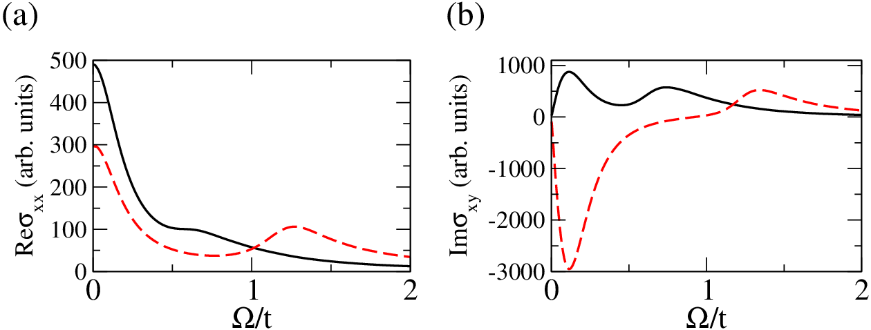
The conductivity $\sigma_{xx}(\Omega)$ in the mean-field theory of the SDW state (Eq (61)) can be obtained in the present leading-order perturbation theory, by simply substituting Eq (20) into various Green’s functions in Eq (36). The vertex corrections are crucial in this derivation; if we had neglected the vertex corrections, we would effectively have neglected the off-diagonal terms in Eq (60) (the terms proportional to $\Delta$). The conductivity in the mean-field SDW state for $\Delta=0.3t$ (solid line) and $\Delta=0.6t$ (dashed line) is shown in Fig 10 (a). The low-frequency parts of these curves are well described by a Drude peak without any anomalous dip. One possible reason is that in the limit $\tau\to\infty$, both $A$ and $G^{R}$ in the mean-field theory are singular, unlike Eqs (9, 16) which are finite due to scattering from spin fluctuations.

In this section, we develop the formalism for calculating the Hall conductivity $\sigma_{xy}$ in the leading order perturbation theory. The calculation of $\sigma_{xy}$ in the self-consistent Born approximation can be found in Refs [44, 45, 46]. At the level of approximation employed here, we find it easier to apply the method developed in Ref [47] to the conductivity diagrams shown in Fig 2 (c). Rewriting the diagrams in Fig 2 (c) in terms of the bare Green’s functions, replacing every electron momentum $\mathbf{p}$ in the loop, according to the minimal coupling rule, by $\mathbf{p}-\frac{e}{c}\mathbf{A}$, and expanding the resulting diagrams to first order in $\mathbf{A}$, we obtain the diagrams shown in Figure 6, in which the intersections where the magnetic field lines denoted by $B$ meet the dressed Green’s functions $G(\mathbf{p},i\epsilon_{n})$ represented by thick solid lines are the dressed magnetic vertices, which are calculated according to Fig 2 (b).

Summing all the diagrams in Figure 6 and expanding the resulting expression up to first order in $\mathbf{k}$, we find that (1) the terms independent of $\mathbf{k}$ vanish, and (2) the terms of first order in $\mathbf{k}$ depends on $\mathbf{B}=i\mathbf{k}\times\mathbf{A}=B\hat{\mathbf{z}}$, signaling gauge invariance. The Hall conductivity on the Matsubara axis can be expressed as

$$\sigma_{xy}(i\Omega_{n})=\frac{\pi}{2}\sigma_{Q}\frac{Ba^{2}}{\Phi_{0}}\frac{1}{i\Omega_{n}}\int\frac{d\mathbf{p}}{(2\pi)^{2}}\Bigl\{S_{1}-S_{2}+S_{3}+S_{4}-S_{5}\Bigr\},$$

(44)

where $\Phi_{0}=\pi\hbar c/e$ is the superconducting flux quantum,

$$S_{1}=T\sum_{i\epsilon_{n}}\bigl(\partial_{y}\Gamma_{p}^{x}v_{p}^{y}-\partial_{y}\Gamma_{p}^{y}v_{p}^{x}\bigr)\bigl(\mathcal{G}\partial_{x}\mathcal{G}(+)-\mathcal{G}(+)\partial_{x}\mathcal{G}\bigr),$$

(45)

$$S_{2}=T\sum_{i\epsilon_{n}}\bigl(\partial_{x}\Gamma_{p}^{x}v_{p}^{y}-\partial_{x}\Gamma_{p}^{y}v_{p}^{x}\bigr)\bigl(\mathcal{G}\partial_{y}\mathcal{G}(+)-\mathcal{G}(+)\partial_{y}\mathcal{G}\bigr),$$

(46)

$$S_{3}=T\sum_{i\epsilon_{n}}\bigl(\Gamma_{p}^{x}v_{p}^{y}-\Gamma_{p}^{y}v_{p}^{x}\bigr)\bigl(\partial_{x}\mathcal{G}(+)\partial_{y}\mathcal{G}-\partial_{x}\mathcal{G}\partial_{y}\mathcal{G}(+)\bigr),$$

(47)

$$S_{4}=g^{2}T^{2}\sum_{i\epsilon_{n}}v_{p}^{y}\mathcal{G}\mathcal{G}(+)\int\frac{d\mathbf{q}}{(2\pi)^{2}}\chi(\mathbf{p}-\mathbf{q})(\varepsilon_{q}^{xx}v_{q}^{y}-\varepsilon_{q}^{xy}v_{q}^{x})\bigl(\mathcal{G}_{0}(+)\mathcal{G}_{0}^{2}-\mathcal{G}_{0}\mathcal{G}_{0}(+)^{2}\bigr),$$

(48)

and

$$S_{5}=g^{2}T^{2}\sum_{i\epsilon_{n}}v_{p}^{x}\mathcal{G}\mathcal{G}(+)\int\frac{d\mathbf{q}}{(2\pi)^{2}}\chi(\mathbf{p}-\mathbf{q})(\varepsilon_{q}^{xy}v_{q}^{y}-\varepsilon_{q}^{yy}v_{q}^{x})\bigl(\mathcal{G}_{0}(+)\mathcal{G}_{0}^{2}-\mathcal{G}_{0}\mathcal{G}_{0}(+)^{2}\bigr).$$

(49)

In writing these equations, we have used short-hand notations: $\mathcal{G}=G(\mathbf{p},i\epsilon_{n})$, $\mathcal{G}(+)=G(\mathbf{p},i\epsilon_{n}+i\Omega_{n})$, $\Gamma_{p}^{x}=\Gamma_{x}(\mathbf{p},i\epsilon_{n},i\epsilon_{n}+i\Omega_{n})$, $\mathcal{G}_{0}=G_{0}(\mathbf{q},i\epsilon_{n})$, and $\mathcal{G}_{0}(+)=G_{0}(\mathbf{q},i\epsilon_{n}+i\Omega_{n})$. Using the spin-fluctuation propagator in the Kampf-Schrieffer model, Eq (19), after a lengthy calculation, we can show that Eq (44) reduces to that in the mean-field theory of the SDW state (Appendix C).[48] The proper treatment of the vertex functions as discussed here is crucial in arriving at this conclusion.

The frequency summation in Eq (44) is standard.[33] The physical observable $\sigma_{xy}(\Omega)$ is obtained by analytical continuation $i\Omega_{n}\to\Omega+i\delta$. The expression for $\mathrm{Im}\sigma_{xy}(\Omega)$ is quite cumbersome. Here, we focus on the results, leaving detailed expressions to Appendix D.

Figures 7 and 8 show $\mathrm{Im}\sigma_{xy}(\Omega)$ calculated from Eq (75) for $1/\tau=0.1t$, $\mu=0.175t$, and various values of $\lambda$ and $\varepsilon_{0}$. The frequency scales in Figures 7 and 8 are selected to highlight the frequency window most relevant to experiments[48] where $\sigma_{xy}$ was measured for $\Omega>0.3t\approx 1000\mathrm{cm}^{-1}$. The low-frequency part ( $\Omega\lesssim 1/\tau$) of $\mathrm{Im}\sigma_{xy}(\Omega)$ suffers from the same difficulty as does $\mathrm{Re}\sigma_{xx}(\Omega)$ due to the perturbative nature of the calculation and we do not show results in this region.

Comparing to Ref [48] suggests that the present calculation captures important features of data. First, $\mathrm{Im}\sigma_{xy}$ can be made negative at low frequencies, although we start with a single-band model with a hole-like Fermi surface. A previous study suggested that the appearance of the negative $\mathrm{Im}\sigma_{xy}$ in electron-doped cuprates is a signature of the long-range spin-density wave order.[48] Our findings here suggest that fluctuating order can also explain this behavior. The vertex corrections shown in Figure 6 are important for this conclusion. We found that $\mathrm{Im}\sigma_{xy}$ remains positive in the entire frequency range, if only the diagrams 1-4, 11, and 12 in Figure 6 are kept and the vertex corrections to magnetic vertices are neglected. Kontani and co-workers, using the FLEX approximation, also emphasized the importance of the magnetic field vertex corrections.[49] As shown in Figure 7, $\mathrm{Im}\sigma_{xy}(\omega)$ has relatively sharp peaks for small $\varepsilon_{0}$ ($\varepsilon_{0}/t=0.05,0.1$ in panel (a), and $\varepsilon_{0}/t=0.1,0.2$ in panel (b)) around $2\Delta_{pg}$, showing precursor effect to that obtained from a mean-field calculation shown in Figure 10 (b). The peak gradually vanishes as $\varepsilon_{0}$ increases. Furthermore, fixing $\lambda$ (or doping $x$) and increasing $\varepsilon_{0}$ (or temperature $T$), $\mathrm{Im}\sigma_{xy}(\Omega)$ increases from negative to positive at low frequencies and decreases at high frequencies. This is qualitatively consistent with the trend observed experimentally in electron-doped cuprates in the underdoped regime.[48] From Figure 8, we see that at fixed $\varepsilon_{0}$, $\mathrm{Im}\sigma_{xy}(\Omega)$ decreases with increasing $\lambda$ (or decreasing $x$) from positive to negative at low frequencies, and increases with increasing $\lambda$ at high frequencies, again qualitatively consistent with data.[48] However, in our study, $\mathrm{Im}\sigma_{xy}(\Omega)$ remains positive at high frequencies, inconsistent with data.[48] More quantitatively, if (following the discussion of the longitudinal conductivity above) we assume that $\lambda/t^{2}=\varepsilon_{0}/t=0.1$ is a reasonable representation of cuprates at $0.12$ electron doping, we see that the predicted zero crossing in $\sigma_{xy}$ occurs at $\Omega\sim 0.15-0.2$eV, again semiquantitatively consistent with data. However, our calculation exhibits more temperature dependence than is found in data.

References

- [1] A. W. Overhauser, Phys. Rev. 128, 1437 (1962).
- [2] N. P. Armitage, P. Fournier, and R. L. Greene, Rev. Mod. Phys. 82, 2421 (2010).
- [3] A. Zimmers, J. M. Tomczak, R. P. S. M. Lobo, N. Bontemps, C. P. Hill, M. C. Barr, Y. Dagan, R. L. Greene, A. J. Millis, and C. C. Homes, EPL (Europhysics Letters) 70, 225 (2005).
- [4] N. Bontemps, R. P. S. M. Lobo, A. F. Santander-syro, and A. Zimmers, Annals of Physics 321, 1547 (2006).
- [5] N. Bontemps, Physica C 460, 162 (2007).
- [6] Y. Dagan, M. M. Qazilbash, C. P. Hill, V. N. Kulkarni, and R. L. Greene, Phys. Rev. Lett. 92, 167001 (2004).
- [7] S. Charpentier, G. Roberge, S. Godin-Proulx, X. Béchamp-Laganière, K. D. Truong, P. Fournier, and P. Rauwel, Physical Review B 81, 104509 (2010).
- [8] G. S. Jenkins, D. C. Schmadel, P. L. Bach, R. L. Greene, X. Béchamp-Laganière, G. Roberge, P. Fournier, and H. D. Drew, Physical Review B 79, 224525 (2009).
- [9] E. M. Motoyama, G. Yu, I. M. Vishik, O. P. Vajk, P. K. Mang, and M. Greven, Nature 445, 186 (2007).
- [10] Y. M. Vilk and A. M. S. Tremblay, Journal of Physics and Chemistry of Solids 56, 1769 (1995).
- [11] Y. M. Vilk and A. M. S. Tremblay, Europhysics Letters 33, 159 (1996).
- [12] P. A. Lee, T. M. Rice, and P. W. Anderson, Phys. Rev. Lett. 31, 462 (1973).
- [13] M. V. Sadovskii, Soviet Physics - JETP 50, 989 (1979).
- [14] J. Schmalian, D. Pines, and B. Stojković, Phys. Rev. B 60, 667 (1999).
- [15] O. Tchernyshyov, Phys. Rev. B 59, 1358 (1999).
- [16] M. V. Sadovskii and N. A. Strigina, Journal of Experimental and Theoretical Physics 95, 526 (2002).
- [17] G. Baym and L. P. Kadanoff, Phys. Rev. 124, 287 (1961).
- [18] G. Baym, Phys. Rev. 127, 1391 (1962).
- [19] O. K. Andersen, A. I. Liechtenstein, O. Jepsen, and F. Paulsen, Journal of Physics and Chemistry of Solids 56, 1573 (1995).
- [20] T. Moriya, Spin Fluctuations in Itinerant Electron Magnetism (Springer-Verlag, 1985).
- [21] J. A. Hertz, Phys. Rev. B 14, 1165 (1976).
- [22] A. J. Millis, Phys. Rev. B 48, 7183 (1993).
- [23] L. B. Ioffe and A. J. Millis, Physics-Uspekhi 41, 595 (1998).
- [24] A. Abanov, A. Chubukov, and J. Schmalian, Advances in Physics 52, 119 (2003).
- [25] I. Paul, C. Pépin, B. N. Narozhny, and D. L. Maslov, Phys. Rev. Lett. 95, 017206 (2005).
- [26] H. v. Löhneysen, A. Rosch, M. Vojta, and P. Wölfle, Reviews of Modern Physics 79, 1015 (pages 61) (2007).
- [27] B. R. Patton and L. J. Sham, Phys. Rev. Lett. 31, 631 (1973).
- [28] S. Takada and E. Sakai, Progress of Theoretical Physics 59, 1802 (1978).
- [29] A. Larkin and A. Varlamov, Theory of fluctuations in superconductors (Clarendon Press, 2005).
- [30] C. Caroli and K. Maki, Phys. Rev. 159, 306 (1967).
- [31] G. Zala, B. N. Narozhny, and I. L. Aleiner, Phys. Rev. B 64, 214204 (2001).
- [32] I. Paul, Phys. Rev. B 77, 224418 (2008).
- [33] G. D. Mahan, Many-Particle Physics (Plenum Press, 1990), 2nd ed.
- [34] A. Abrikosov, L. P. Gorkov, and I. E. Dzyaloshinskii, Methods of Quantum Field Theory in Statistical Physics (Prentice Hall, 1963).
- [35] B. L. Altshuler, L. B. Ioffe, and A. J. Millis, Phys. Rev. B 50, 14048 (1994).
- [36] A. J. Millis, H. Monien, and D. Pines, Phys. Rev. B 42, 167 (1990).
- [37] T. Moriya and K. Ueda, Advances in Physics 49, 555 (2000).
- [38] S. Sachdev, Quantum Phase Transitions (Cambridge University Press, 1999).
- [39] A. P. Kampf and J. R. Schrieffer, Phys. Rev. B 42, 7967 (1990).
- [40] A. V. Chubukov and D. K. Morr, Physics Reports 288, 355 (1997).
- [41] J. R. Schrieffer, Theory of superconductivity (Perseus Books, 1999).
- [42] Z. Koba, N. Mugibayashi, and S. Nakai, Progress of Theoretical Physics 6, 322 (1951).
- [43] H. Monien, Phys. Rev. Lett. 87, 126402 (2001).
- [44] H. Fukuyama, H. Ebisawa, and Y. Wada, Progress of Theoretical Physics 42, 494 (1969).
- [45] H. Fukuyama, Progress of Theoretical Physics 42, 1284 (1969).
- [46] H. Kohno and K. Yamada, Progress of Theoretical Physics 80, 623 (1988).
- [47] B. L. Altshuler and A. G. Aronov, Electron-Electron Interactions in Disordered Systmes (North-Holland, 1985), chap. Electron-electron interactions in disordered systems, pp. 1–154, Modern Problems in Condensed Matter Sciences, ISBN 0-444-86916-6.
- [48] A. Zimmers, L. Shi, D. C. Schmadel, W. M. Fisher, R. L. Greene, H. D. Drew, M. Houseknecht, G. Acbas, M.-H. Kim, M.-H. Yang, et al., Physical Review B 76, 064515 (2007).
- [49] H. Kontani, K. Kanki, and K. Ueda, Phys. Rev. B 59, 14723 (1999).
- [50] G. S. Jenkins, D. C. Schmadel, P. L. Bach, R. L. Greene, X. Béchamp-Laganière, G. Roberge, P. Fournier, H. Kontani, and H. D. Drew, Phys. Rev. B 81, 024508 (2010).
- [51] P. Voruganti, A. Golubentsev, and S. John, Phys. Rev. B 45, 13945 (1992).