On the Energy Efficiency of LT Codes in
Proactive Wireless Sensor Networks
Thanks: Manuscript received April 1, 2010; revised June 28, 2010 and September 22, 2010;
accepted November 9, 2010. The associate editor coordinating the review of this
manuscript and approving it for publication was Prof. Shengli Zhou.Thanks: Copyright (c) 2010 IEEE. Personal use of this material is permitted.
However, permission to use this material for any other purposes must be obtained
from the IEEE by sending a request to pubs-permissions@ieee.org.Thanks: J. Abouei is with the Department of Electrical Engineering,
Yazd University, Yazd, Iran (e-mail: abouei@yazduni.ac.ir). Thanks: J. D. Brown is with the DRDC Ottawa, Ottawa, ON, Canada. He completed his
Ph.D. in ECE at University of Toronto (e-mail:
david_jw_brown@yahoo.com).Thanks: K. N. Plataniotis, and S. Pasupathy are with the Edward S.
Rogers Sr. Department of Electrical and Computer Engineering,
University of Toronto, Toronto, ON M5S 3G4, Canada (e-mails:
{kostas, pas}@comm.utoronto.ca).Thanks: The material in this paper was presented
in part at the QBSC’2010 conference, Kingston, Canada, May 2010 [1].
The work of J. Abouei was performed when he was with the Department of Electrical
and Computing Engineering, University of Toronto, Toronto, ON M5S 3G4, Canada.
The work was supported in part by an Ontario Research Fund (ORF) project
entitled “Self-Powered Sensor Networks”.
Abstract
This paper presents an in-depth analysis on the energy efficiency of Luby Transform (LT) codes with Frequency Shift Keying (FSK) modulation in a Wireless Sensor Network (WSN) over Rayleigh fading channels with path-loss. We describe a proactive system model according to a flexible duty-cycling mechanism utilized in practical sensor apparatus. The present analysis is based on realistic parameters including the effect of channel bandwidth used in the IEEE 802.15.4 standard, active mode duration and computation energy. A comprehensive analysis, supported by some simulation studies on the probability mass function of the LT code rate and coding gain, shows that among uncoded FSK and various classical channel coding schemes, the optimized LT coded FSK is the most energy-efficient scheme for distance greater than the pre-determined threshold level , where the optimization is performed over coding and modulation parameters. In addition, although the optimized uncoded FSK outperforms coded schemes for , the energy gap between LT coded and uncoded FSK is negligible for compared to the other coded schemes. These results come from the flexibility of the LT code to adjust its rate to suit instantaneous channel conditions, and suggest that LT codes are beneficial in practical low-power WSNs with dynamic position sensor nodes.
Index Terms:
Wireless sensor networks, energy efficiency, LT codes, green modulation, FSK.I Introduction
Wireless Sensor Networks (WSNs) have been recognized as a new generation of ubiquitous computing systems to support a broad range of applications, including monitoring, health care and tracking environmental pollution levels. Minimizing the total energy consumption in both circuit components and RF signal transmission is a crucial challenge in designing a WSN. Central to this study is to find energy-efficient modulation and coding schemes in the physical layer of a WSN to prolong the sensor lifetime [2, 3]. For this purpose, energy-efficient modulation/coding schemes should be simple enough to be implemented by state-of-the-art low-power technology, but still robust enough to provide the desired service. Furthermore, since sensor devices frequently switch from sleep mode to active mode, modulation and coding circuits should have fast start-up times [4] along with the capability of transmitting packets during a pre-assigned time slot before new sensed packets arrive. In addition, a WSN needs a powerful channel coding scheme (when the distance between nodes exceeds a certain threshold level) to protect transmitted data against the unpredictable and harsh nature of channels. We refer to these low-complexity and low-energy consumption approaches in WSNs providing proper link reliability as Green Modulation/Coding (GMC) schemes.
There have been several recent works on the energy efficiency of various modulation/ coding schemes in WSNs (see e.g., [2, 5, 6]). Tang et al. [5] compare the power efficiency of PPM and FSK in a WSN over fading channels with path-loss without considering the effect of channel coding. Reference [7] investigates the energy efficiency of BCH and convolutional codes with FSK for the optimal packet length in a point-to-point WSN. It is shown in [7] that BCH codes can improve energy efficiency compared to the convolutional code for the optimal fixed packet size. Liang et al. [8] investigate the energy efficiency of uncoded FSK modulation in a WSN, where multiple senders transmit their data to a central node in a Frequency-Division Multiple Access (FDMA) fashion. Reference [9] presents the hardware implementation of the Forward Error Correction (FEC) encoder in IEEE 802.15.4 WSNs, which employs parallel processing to achieve a low processing latency and energy consumption.
Most of the pioneering work on energy-efficient modulation/coding, including research in [5, 7], has focused only on minimizing the energy consumption of transmitting one bit, ignoring the effect of bandwidth and transmission time duration. In a practical WSN however, it is shown that minimizing the total energy consumption depends strongly on the active mode duration and the channel bandwidth. References [2], [6] and [10] address this issue in a point-to-point WSN, where a sensor node transmits an equal amount of data per time unit to a designated sink node. In [2], the authors show that uncoded MQAM is more energy-efficient than uncoded MFSK for short-range applications, while using convolutional coded MFSK over AWGN is desirable for longer distances. This line of work is further extended in [6] by evaluating the energy consumption per information bit of a WSN for Reed Solomon (RS) Codes and various modulation schemes over AWGN channels with path-loss. In [2] and [6], the authors do not consider the effect of multi-path fading.
More recently, the attention of researchers has been drawn to deploying rateless codes (e.g., Luby Transform (LT) code [11]) in WSNs due to the significant advantages of these codes in erasure channels. For instance in [12], the authors present a scheme for cooperative error control coding using rateless and Low-Density Generator-Matrix (LDGM) codes in a multiple relay WSN. However, investigating the energy efficiency of rateless codes in WSNs with low-energy modulations over realistic fading channel models has received little attention. To the best of our knowledge, there is no existing analysis on the energy efficiency of rateless coded modulation that considers the effect of channel bandwidth and active mode duration on the total energy consumption in a proactive WSN. This paper addresses this issue and presents the first in-depth analysis of the energy efficiency of LT codes with FSK, known as green modulation as described in [10]. The present analysis is based on a realistic model in proactive WSNs operating over a Rayleigh fading channel with path-loss. In addition, we obtain the probability mass function of the LT code rate and the corresponding coding gain, and study their effects on the energy efficiency of the WSN. This study uses the classical BCH and convolutional codes (as reference codes), utilized in IEEE standards, for comparative evaluation. Numerical results, supported by some experimental setup on the computation energy, show that the optimized LT coded FSK scheme is the most energy-efficient scheme for distance greater than the threshold level . In addition, although the optimized uncoded FSK outperforms coded schemes for , the energy gap between LT coded and uncoded FSK is negligible for compared to the other coded schemes. This result comes from the simplicity and flexibility of the LT codes, and suggests that LT codes are beneficial in practical low-power WSNs with dynamic position sensor nodes.
The rest of the paper is organized as follows. In Section II, the proactive system model over a realistic wireless channel is described. The energy consumption of both circuits and signal transmission of uncoded MFSK modulation is analyzed in Section III. Design of LT codes and the energy efficiency of the LT coded MFSK are presented in Section IV. Section V provides some numerical evaluations using some classical channel codes as well as realistic models to confirm our analysis. Also, some design guidelines for using LT codes in practical WSN applications are presented. Finally in Section VI, an overview of the results and conclusions are presented.
For convenience, we provide a list of key mathematical symbols used in this paper in Table I. For simplicity of notation, we use the superscripts ‘BC’, ‘CC’ and ‘LT’ for BCH, convolutional and LT codes, respectively. We use , and for energy, power and time parameters, respectively. Also, we use the subscript “” to distinguish coding parameters from the uncoded ones.
| : Channel bandwidth | : Number of bits in each symbol |
| : Transmission distance | : Energy of transmitted signal |
| : Expectation operator | : Total energy consumption |
| : Constellation size | : Fading channel coefficient |
| : Number of sensed message | : Path loss gain |
| : Codeword block length | : Output-node degree distribution |
| : Bit error rate | : Circuit power consumption |
| : pmf of LT code rate | : Power of transmitted signal |
| : Code rate | : Active mode duration |
| : Path-loss exponent | : Transient mode duration |
| : Symbol duration | |
| : Coding gain | : Instantaneous SNR |
II System Model and Assumptions
We consider a proactive wireless sensor system, in which a sensor node transmits an equal amount of data per time unit to a designated sink node. Such a proactive sensor system is typical of many environmental applications such as sensing temperature, humidity and level of contamination [13]. We assume a non real-time service application where the data transmission between the sensor and the sink nodes does not have tight constraint on delay. The sensor and sink nodes synchronize with one another and operate in a real-time based process as depicted in Fig 1. During active mode period , the sensed analog signal is first digitized by an Analog-to-Digital Converter (ADC), and an -bit message sequence is generated, where is assumed to be fixed, and , . The bit stream is then sent to the channel encoder. The encoding process begins by dividing the uncoded message into blocks of equal length denoted by , , where is the length of any particular , and is assumed to be divisible by . Each block is encoded by a pre-determined channel coding scheme to generate a coded bit stream , , with block length , where is either a fixed value (e.g., for block and convolutional codes) or a random variable (e.g., for LT codes).

The coded stream is then modulated by the FSK scheme and transmitted to the sink node. Finally, the sensor node returns to sleep mode, and all the circuits are shutdown for sleep mode duration . We denote as the transient mode duration consisting of the switching time from sleep mode to active mode (i.e., ) plus the switching time from active mode to sleep mode (i.e., ), where is short enough to be negligible. Under the above considerations, the sensor/sink nodes have to process one entire -bit message during , where is fixed and .
Since sensor nodes in a typical WSN are densely deployed, the distance between nodes is normally short. Thus, the total circuit power consumption, defined by , is comparable to the RF transmit power consumption denoted by , where and represent the circuit power consumptions for the sensor and sink nodes, respectively. Taking these into account, the total energy consumption during the active mode period, denoted by , is given by . Also, the power consumption during the sleep mode duration is much smaller than the power consumption in the active mode (due to the low sleep mode leakage current) to be negligible. As a result, we have the following definition.
Definition 1
(Performance Metric): The energy efficiency, referred to as the performance metric of the proposed WSN, can be measured by the total energy consumption in each period corresponding to -bit message as follows:
| (1) |
where is the circuit power consumption during the transient mode period.
We use (1) to investigate and compare the energy efficiency of uncoded and coded FSK for various channel coding schemes in the subsequent sections.
Channel Model: The choice of low transmission power in WSNs results in several consequences to the channel model. It is shown by Friis [14] that a low transmission power implies a small range. For short-range transmission scenarios, the root mean square (rms) delay spread is in the range of nanoseconds [15] which is small compared to the symbol duration s obtained from the bandwidth KHz in the IEEE 802.15.4 standard, where is the constellation size of M-ary FSK [16, pp. 114-115] and [17, p. 49]. Thus, it is reasonable to expect a flat-fading channel model for WSNs. In addition, many transmission environments include significant obstacle and structural interference by obstacles (such as wall, doors, furniture, etc), which leads to reduced Line-Of-Sight (LOS) components. This behavior suggests a Rayleigh fading channel model. Under the above considerations, the channel model between the sensor and sink nodes is assumed to be Rayleigh flat-fading with path-loss. This assumption is used in many works in the literature (e.g., see [5] for WSNs). For this model, we assume that the channel is constant during the transmission of a codeword, but may vary from one codeword to another. We denote the fading channel coefficient corresponding to symbol as , where the amplitude is Rayleigh distributed with probability density function (pdf) , where [18].
To model the path-loss of a link where the transmitter and receiver are separated by distance , let denote and as the transmitted and the received signal powers, respectively. For a -power path-loss channel, the channel gain factor is given by , where is the gain margin which accounts for the effects of hardware process variations, background noise and is the gain factor at meter which is specified by the transmitter and receiver antenna gains and , and wavelength (e.g., [2]). As a result, when both fading and path-loss are considered, the instantaneous channel coefficient becomes . Denoting as the transmitted signal with energy , the received signal at the sink node is given by , where is AWGN at the sink node with two-sided power spectral density given by . Under the above considerations, the instantaneous Signal-to-Noise Ratio (SNR) corresponding to symbol can be computed as . Under the assumption of a Rayleigh fading channel model, is chi-square distributed with 2 degrees of freedom and with pdf , where denotes the average received SNR.
III Energy Consumption of Uncoded Scheme
In this section, we consider the uncoded M-ary FSK modulation where orthogonal carriers can be mapped into bits. Among various sinusoidal carrier-based modulation techniques, FSK has been found to provide a good compromise between simple radio architecture, low-power consumption, and requirements on linearity of the modulation scheme [10, 19, 2]. Also, this scheme is used in some IEEE standards (e.g., [20]). Since we have bits during each symbol period , we can write
| (2) |
where comes from the bandwidth with the minimum carrier separation for MFSK with the non-coherent detector [16, pp. 114-115]. It is shown in [10] that the transmit energy consumption per each symbol for an uncoded MFSK with non-coherent detector is obtained as
| (3) | |||||
where comes from the fact that the relationship between the average Symbol Error Rate (SER) and the average Bit Error Rate (BER) of MFSK is given by [18, p. 262]. As a result, the output energy consumption of transmitting -bit during of an uncoded MFSK is computed from (2) as follows:
| (5) | |||||
For the sensor node with uncoded MFSK, we denote the power consumption of frequency synthesizer, filters and power amplifier as , and , respectively. In this case, the circuit power consumption of the sensor node with uncoded MFSK can be obtained as
| (6) |
where with [2], [5]. In addition, the power consumption of the sink circuitry with uncoded MFSK scheme can be obtained as
| (7) |
where , , , and denote the power consumption of Low-Noise Amplifier (LNA), filters, envelop detector, IF amplifier and ADC, respectively [10]. Since, the power consumption during transient mode period is governed by the frequency synthesizer in both transmitter and the receiver [4], the energy consumption during is obtained as [2]. Substituting (2) and (5) in (1), the total energy consumption of an uncoded MFSK for transmitting -bit information in each period for a given is obtained as
| (8) | |||||
For energy optimal designs, the impact of channel coding on the energy efficiency of the proposed WSN must be considered as well. It is a well known fact that channel coding is a classical approach used to improve the link reliability along with the transmitter energy saving due to providing the coding gain [18]. However, the energy saving comes at the cost of extra energy spent in transmitting the redundant bits in codewords as well as the additional energy consumption in the process of encoding/decoding. For a specific transmission distance , if these extra energy consumptions outweigh the transmit energy saving due to the channel coding, the coded system would not be energy-efficient compared with an uncoded system. In the subsequent sections, we will argue the above problem and determine at what distance use of specific channel coding becomes energy-efficient compared to uncoded systems. In particular, we will show in Section V that the LT coded modulation surpasses this distance constraint in the proposed WSN.
IV Energy Consumption Analysis of LT Coded Modulation
In this section, we present the first in-depth analysis on the energy efficiency of LT coded modulation for the proposed proactive WSN. To get more insight into how channel coding affects the circuit and RF signal energy consumptions in the system, we modify the energy concepts in Section III, in particular, the total energy consumption expression in (8) based on the coding gain, code rate and the computation energy. We further present the first study on the tradeoff between LT code rate and coding gain required to achieve a certain BER, and the effect of this tradeoff on the total energy consumption of LT coded MFSK for different transmission distances.
IV-A Energy Efficiency of Coded System
For an arbitrary channel coding scheme, each -bit message is encoded into the codeword with block length and code rate . In this case, the number of transmitted bits in is increased from -bit uncoded message to bits coded one. To compute the energy consumption of coded scheme, we use the fact that channel coding reduces the required average SNR value to achieve a given BER (i.e., the same BER as uncoded one). Taking this into account, the proposed WSN benefits in transmission energy saving of coded modulation specified by , where is the coding gain11 1 Denoting and as the average SNR of uncoded and coded schemes, respectively, the coding gain (expressed in dB) is defined as the difference between the values of and required to achieve a certain BER, where . of the utilized coded MFSK. It should be noted that the cost of this energy saving is the bandwidth expansion . In order to keep the bandwidth of the coded system the same as that of the uncoded case, we must keep the information transmission rate constant, i.e., the symbol duration of uncoded and coded MFSK would be the same. However, the active mode duration increases from in the uncoded system to
| (9) |
for the coded case. Thus, one would assume that the total time increases to for the coded scenario. It is worth mentioning that the active mode period in the coded case is upper bounded by . As a result, the maximum constellation size , denoted by , for the coded MFSK is calculated by , which is approximately the same as that of the uncoded case.
| (11) | |||||
| (12) | |||||
| (13) |
We denote and as the computation energy of the encoder and decoder for each information bit, respectively. Thus, the total computation energy cost of the coding components for bits is obtained as . Substituting () in , and using (6), (7) and (9), the total energy consumption of transmitting bits in each period for an arbitrarily coded MFSK, and a given is obtained as
| (10) | |||||
To make a fair comparison between the uncoded and coded modulation, we use the same BER and drop the subscript “” for in the coded case. Thus, the optimization goal is to minimize the objective function over modulation and coding parameters. This is achieved by finding the optimum constellation size under the constraint for a specific channel coding scheme, and then minimize over the coding parameters.
For the above optimization problem, we consider two scenarios: fixed-rate codes (e.g., BCH and convolutional codes), and variable rate codes (e.g., LT codes). To find the optimum for a given fixed-rate code, we prove that (10) is a monotonically increasing function of for every value of and . Since and are fixed and is independent of , it is concluded that the second term in (10) is a monotonically increasing function of . Also, from the first term in (10), we have (11)-(13) in the top of this page, where comes from the approximation , and the fact that scales as . Also, follows from the approximation . On the other hand, it is shown in [18] that for MFSK is a decreasing function of . Thus, it is concluded from (13) that the first term in (10) is also a monotonically increasing function of . As a result, the minimum total energy consumption for a given fixed-rate code is achieved at .
In the next section, we evaluate the above optimization problem for the LT codes using some simulation studies on the probability mass function of the LT code rate and coding gain. We show that the LT code parameters depend strongly on the constellation size and exhibit different trends over fixed-rate codes. In addition, we present some beneficial uses of LT codes over block and convolutional codes in managing the energy consumption for different channel realizations.
IV-B Energy Optimality of LT Codes
LT codes are the first class of Fountain codes which usually specified by the number of input bits and the output-node degree distribution . Without loss of generality and for ease of our analysis, we assume that a single -bit message is encoded to codeword . Each single coded bit is generated based on the encoding protocol proposed in [11]: randomly choose a degree from , using a uniform distribution, randomly choose distinct input bits, and calculate the encoded bit as the XOR-sum of these bits. The above encoding process defines a bipartite graph connecting encoded nodes to input nodes (see, e.g., Fig. 2). It is seen that the LT encoding process is extremely simple and has very low energy consumption. Unlike block and convolutional codes, in which the codeword block length is fixed, for the above LT code, is a variable parameter, resulting in a random variable LT code rate . More precisely, is the last bit generated at the output of LT encoder before receiving the acknowledgement signal from the sink node indicating termination of a successful decoding process. This inherent property of LT codes means they can vary their codeword block lengths to adapt to any wireless channel condition between the sensor and the sink nodes.

To describe the output-node degree distribution used in this work, let , , denote the probability that an output node has degree . Following the notation of [21], the output-node degree distribution of an LT code has the polynomial form with the property that . Typically, optimizing the output-node degree distribution for a specific wireless channel model is a crucial task in designing LT codes. In fact, for wireless fading channels, it is still an open problem, what the “optimal” is. In this work, we use the following output-node degree distribution which was optimized for a BSC using a hard-decision decoder [22]:
| (11) | |||||
The LT decoder at the sink node can recover the original -bit message with high probability after receiving any bits in its buffer, where depends upon the LT code design [21]. For this recovery process, the LT decoder needs to correctly reconstruct the bipartite graph of an LT code. One practical approach suitable for the proposed WSN model is that the LT encoder and decoder use identical pseudo-random generators with a common seed value which may reduce the complexity further. In this work, we assume that the sink node recovers -bit message using a simple hard-decision “ternary message passing” decoder in a nearly identical manner to the “Algorithm E” decoder in [23] for Low-Density Parity-Check (LDPC) codes22 2 Description of the ternary message passing decoding is out of scope of this work, and the reader is referred to Chapter 4 in [22] for more details.. Also, the degree distribution in (11) was optimized for a ternary decoder in a BSC and we are aware of no better for the ternary decoder in Rayleigh fading channels.
Unlike fixed-rate codes in which the active mode duration of coded MFSK is fixed, for the LT coded MFSK, we have a non-fixed value for
| (12) |
An interesting point raised from (12) is that is a function of the random variable which results in an inherent adaptive duty-cycling for power management in each channel condition without any channel state information fed back from the sink node to the sensor node. Recalling from (10), we have
where the main goal is to minimize over and the coding parameters. Toward this goal, we first compute the LT code rate and the corresponding LT coding gain. Let us begin with the case of asymptotic LT code rate, where the number of input bits goes to infinity. It is shown that the LT code rate is obtained asymptotically as a fixed value of for large values of , where and represent the average degree of the output and the input nodes in the bipartite graph, respectively (see Appendix I for the proof).
When using finite- LT codes, we are treating the channel as static over one block length. In this case, the rate of the LT code for any block can be chosen to achieve the desired performance for that block. More precisely, for the particular block we are concerned with, the receiver could evaluate the channel instantaneous SNR, and then determine how many code bits it needs to collect in order to achieve its given BER target, thus essentially dynamically selecting its rate. For the next block, the receiver would once again evaluate the (new) instantaneous channel SNR and adjust its rate accordingly to collect more or fewer bits.
It should be noted that there is no (currently known) explicit equation governing the relationship between the instantaneous SNR and the required number of decoding bits for an LT code. In this work, we determine the necessary number of decoding bits in each case through simulation, as described below:
- i)
We decide upon a “target BER” for the decoded bits - e.g., the decoded message needed an average BER of or better.
- ii)
Based on the assumption that instantaneous SNR is constant over at least one block we perform the following steps for a large range of possible instantaneous SNR:
- Determine through numerical simulation the decoded BER using the LT code rate .
- If the decoded BER is greater than the target BER, then we reduce the LT code rate and try again.
- Repeat the above step until the decoded BER is less than the target BER.
- iii)
At this point, for the given LT degree distribution, decoder, and SNR we can identify the highest LT code rate that will yield the target BER or better.
Armed with this information (computed ahead of time), a receiver can determine the appropriate rate at which to operate and hence determine how many bits it must collect for a given instantaneous SNR. This is also based on the common assumption that the receiver is capable of estimating the instantaneous SNR.
Based on the above arguments and for any given average SNR, the LT code rate is described by either a probability mass function (pmf) or a probability density function (pdf) denoted by . Because it is difficult to get a closed-form expression of , we use a discretized numerical method to calculate the pmf , , for different values of . We plot the pmfs of the LT code rate in Fig. 3 for and various average SNR 33 3 It should be noted that the average SNR is expressed in terms of , where represents the transmit energy per bit. over a Rayleigh fading channel model. It is observed that for lower average SNRs the pmfs are larger in the lower rate regimes (i.e., the pmfs spend more time in the low rate region). Also, all pmfs exhibit quite a spike for the highest rate, which makes sense since once the instantaneous SNR hits a certain critical value, the codes will always decode with a high rate. Also, Fig. 4 illustrates the pmf of LT code rates for various constellation size and for average SNR equal to 16 dB. It can be seen that as increases, the rate of the LT code tends to have a pmf with larger values in the lower rate regions.


Table II illustrates the average LT code rates and the corresponding coding gains of LT coded MFSK using in (11), for and given . The average rate for a certain average SNR is obtained by integrating the pmf over the rates from to . To get more insight into the relationship between the LT code rate and coding gain, we plot the results of Table II in Fig. 5. It is observed that the LT code is able to provide a huge coding gain given , but this gain comes at the expense of a very low average code rate, which means many additional code bits need to be sent. This results in higher energy consumption per information bit. In contrast to the fixed-rate codes in which the coding gain decreases when grows, the LT coding gains display different trends in terms of as illustrated in Table II. Thus, in contrast with fixed-rate codes, is not necessarily a monotonically increasing function of . In the next section, we evaluate numerically in terms of the optimized modulation and coding parameters compared to the uncoded and the fixed-rate codes.

An interesting point extracted from Table II is the flexibility of the LT code to adjust its rate (and its corresponding coding gain) to suit instantaneous channel conditions in WSNs. For instance in the case of favorable channel conditions, the LT coded MFSK is able to achieve with dB, which is similar to the case of uncoded MFSK, i.e., . The effect of LT code rate flexibility on the total energy consumption is also observed in the simulation results in the subsequent section.
| M=2 | M=4 | M=8 | M=16 | ||||||
| Average | Coding | Average | Coding | Average | Coding | Average | Coding | ||
| (dB) | Code Rate | Gain (dB) | (dB) | Code Rate | Gain (dB) | Code Rate | Gain (dB) | Code Rate | Gain (dB) |
| 5 | 0.2560 | 25 | 0 | 0.0028 | 33.87 | 0.0012 | 36.46 | 0.0012 | 38.48 |
| 6 | 0.3174 | 24 | 2 | 0.0140 | 31.87 | 0.0024 | 34.46 | 0.0012 | 36.48 |
| 7 | 0.3819 | 23 | 4 | 0.0460 | 29.87 | 0.0095 | 32.46 | 0.0021 | 34.48 |
| 8 | 0.4475 | 22 | 6 | 0.1100 | 27.87 | 0.0330 | 30.46 | 0.0086 | 32.48 |
| 9 | 0.5120 | 21 | 8 | 0.2100 | 25.87 | 0.0870 | 28.46 | 0.0320 | 30.48 |
| 10 | 0.5738 | 20 | 10 | 0.3300 | 23.87 | 0.1800 | 26.46 | 0.0870 | 28.48 |
| 11 | 0.6315 | 19 | 12 | 0.4600 | 21.87 | 0.3000 | 24.46 | 0.1800 | 26.48 |
| 12 | 0.6840 | 18 | 14 | 0.5900 | 19.87 | 0.4400 | 22.46 | 0.3100 | 24.48 |
| 13 | 0.7307 | 17 | 16 | 0.7000 | 17.87 | 0.5700 | 20.46 | 0.4500 | 22.48 |
| 14 | 0.7716 | 16 | 18 | 0.7800 | 15.87 | 0.6800 | 18.46 | 0.5800 | 20.48 |
| 15 | 0.8067 | 15 | 20 | 0.8500 | 13.87 | 0.7700 | 16.46 | 0.6900 | 18.48 |
| 16 | 0.8365 | 14 | 22 | 0.8900 | 11.87 | 0.8400 | 14.46 | 0.7800 | 16.48 |
| 17 | 0.8614 | 13 | 24 | 0.9200 | 9.87 | 0.8800 | 12.46 | 0.8400 | 14.48 |
| 18 | 0.8821 | 12 | 26 | 0.9400 | 7.87 | 0.9100 | 10.46 | 0.8800 | 12.48 |
| 19 | 0.8991 | 11 | 28 | 0.9500 | 5.87 | 0.9300 | 8.46 | 0.9200 | 10.48 |
| 20 | 0.9130 | 10 | 30 | 0.9600 | 3.87 | 0.9500 | 6.46 | 0.9400 | 8.48 |
| 22 | 0.9333 | 8 | 32 | 0.9600 | 1.87 | 0.9500 | 4.46 | 0.9500 | 6.48 |
| 24 | 0.9466 | 6 | 34 | 0.9600 | -0.13 | 0.9600 | 2.46 | 0.9500 | 4.48 |
| 26 | 0.9551 | 4 | 36 | 0.9700 | -2.13 | 0.9600 | 0.46 | 0.9600 | 2.48 |
| 28 | 0.9606 | 2 | 38 | 0.9700 | -4.13 | 0.9700 | -1.54 | 0.9600 | 0.48 |
| 30 | 0.9640 | 0 | 40 | 0.9700 | -6.13 | 0.9700 | -3.54 | 0.9700 | -1.52 |
V Numerical Evaluations
In this section, we present some numerical evaluations using realistic parameters from the IEEE 802.15.4 standard and state-of-the art technology to confirm the energy efficiency analysis of uncoded and coded MFSK modulations discussed in Sections III and IV.
V-A Experimental Setup
We assume that MFSK operates in the carrier frequency 2.4 GHz Industrial Scientist and Medical (ISM) unlicensed band utilized in the IEEE 802.15.14 standard [17]. According to the FCC 15.247 RSS-210 standard for United States/Canada, the maximum allowed antenna gain is 6 dBi [24]. In this work, we assume that dBi. Thus for the 2.4 GHz, , where m. We assume that in each period , the data frame bytes (or equivalently bits) is generated, where is assumed to be 1.4 s. The channel bandwidth is set to the KHz, according to IEEE 802.15.4 [17, p. 49]. It is concluded from that (or equivalently ) for MFSK. Table III summarizes the system parameters for simulation44 4 To make a fair comparison between the energy consumption of different communication schemes, the bandwidth and the BER are assumed to be the same for all the schemes. [2, 5, 25, 4]. The results in Tables II are also used to compare the energy efficiency of uncoded and coded MFSK schemes.
| KHz | dB | mw |
|---|---|---|
| dB | mw | mw |
| dB | mw | mw |
| mw | mw | |
| sec |
In order to estimate the computation energy of a specific channel coding, we use the ARM7TDMI core which is the industry’s most widely used 32-bit embedded RISC microprocessor for an accurate power simulation [26]. For the energy and power calculations, the relations and are used, where
-
number of operations per block.
-
number of clock cycles on operations.
-
total dynamic power consumption per Hertz (W/Hz) of a single calculation cycle.
In addition, for the purpose of comparative evaluation, we use some classical BCH codes with -error correction capability, and convolutional codes with the constraint length . These codes are widely utilized in IEEE standards [27, 28]. We use hard-decision prior to decoding for the BCH and convolutional codes. The main reason for using the hard-decision here is to make a fair comparison to the LT code, since this code involved a hard-decision in ternary decoder.
V-B Optimal Configuration
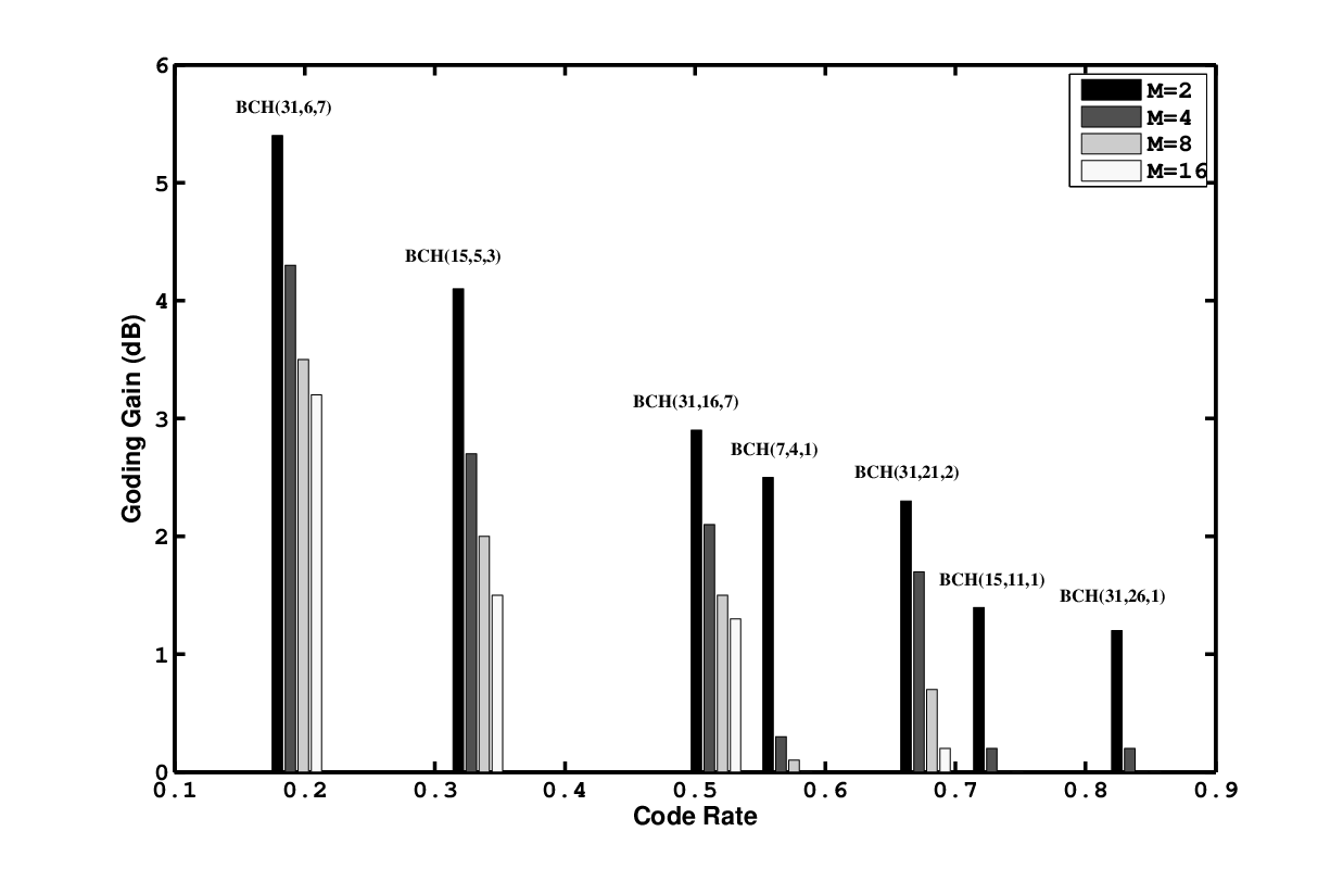
As a starting point, we obtain the coding gain of some practical BCH and convolutional codes with MFSK for different constellation size and given in Table IV. We observe from Table IV that there is a tradeoff between coding gain and decoder complexity for the BCH codes. In fact, achieving a higher coding gain for a given , requires a more complex decoding process, (i.e., higher ) with more circuit power consumption. In addition, it is seen from Fig. 6 that the coding gain of the BCH code is a monotonically decreasing function of as expected. For a given , the convolutional codes with lower rates and higher constraint lengths achieve greater coding gains. In contrast to [2], where the authors assume a fixed convolutional coding gain for every value of , it is observed that the coding gain of convolutional coded MFSK is a monotonically decreasing function of . By comparing the results in Table II with those in Table IV for BCH and convolutional codes, one observes that LT codes outperform the other coding schemes in energy saving at comparable rates.
| BCH Code | M=2 | M=4 | M=8 | M=16 | M=32 | M=64 | |
|---|---|---|---|---|---|---|---|
| BCH | 0.571 | ||||||
| BCH | 0.733 | ||||||
| BCH | 0.467 | ||||||
| BCH | 0.333 | ||||||
| BCH | 0.839 | ||||||
| BCH | 0.677 | ||||||
| BCH | 0.516 | ||||||
| BCH | 0.355 | ||||||
| BCH | 0.194 | ||||||
| Convolutional Code | M=2 | M=4 | M=8 | M=16 | M=32 | M=64 | |
| trel | 0.500 | ||||||
| trel | 0.500 | ||||||
| trel | 0.333 | ||||||
| trel | 0.667 | ||||||
| trel | 0.667 |
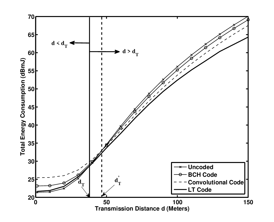
Fig. 7 shows the total energy consumption versus distance for the optimized BCH, convolutional and LT coded MFSK schemes, compared to the optimized uncoded MFSK for . The optimization is done over and the parameters of coding scheme. Simulation results show that for less than the threshold level m, the total energy consumption of optimized uncoded MFSK is less than that of the coded MFSK schemes. However, the energy gap between LT coded and uncoded MFSK is negligible compared to the other coded schemes as expected. For , the LT coded MFSK scheme is more energy-efficient than uncoded and other coded MFSK schemes. Also, it is observed that the energy gap between LT and convolutional coded MFSK increases when the distance grows. This result comes from the high coding gain capability of LT codes which confirms our analysis in Section IV. The threshold level (for LT code) or (for BCH and convolutional codes) are obtained when the total energy consumptions of coded and uncoded systems become equal. For instance, using , and the equality between (8) and (10) for uncoded and convolutional coded MFSK, we have
| (13) |
where
| (14) | |||||
| (15) |
| (16) |
It should be noted that the above threshold level imposes a constraint on the design of the physical layer of some wireless sensor networking applications, in particular dynamic WSNs. To obtain more insight into this issue, let assume that the location of the sensor node is changed every time unit, where is the channel coherence time. For the moment, let us assume that the sensor node aims to choose either a fixed-rate coded or an uncoded MFSK based on the distance between sensor and sink nodes. According to the results in Fig. 7, it is revealed that using fixed-rate channel coding is not energy efficient for short distance transmission (i.e., ), while for , convolutional coded MFSK is more energy-efficient than other schemes. For this configuration, the sensor node must have the capability of an adaptive coding scheme for each distance . However, as discussed previously, the LT codes can adjust their rates for each channel condition and have (with a good approximation) minimum energy consumption for every distance . This indicates that LT codes can surpass the above distance constraint for WSN applications with dynamic position sensor nodes over Rayleigh fading channels. This characteristic of LT codes results in reducing the complexity of the network design as well. Of interest is the strong benefits of using LT coded MFSK compared with the coded modulation schemes in [2, 6]. In contrast to classical fixed-rate codes used in [2, 6], the LT codes can vary their block lengths to adapt to any channel condition in each distance . Unlike [2] and [6], where the authors consider fixed-rate codes over an AWGN channel model, we considered a Rayleigh fading channel which is a general model in practical WSNs. The simplicity and flexibility advantages of LT codes with an MFSK scheme make them the preferable choice for wireless sensor networks, in particular for WSNs with dynamic position sensor nodes.
Remark 1: As discussed previously, the proposed LT coded scheme benefits in adjusting the coding parameters in each channel realization or equivalently each distance to minimize the total energy consumption. As we will show shortly, this comes from a variable transmission time process which adaptively controls the power consumption of the proposed scheme. To address this issue, we plot the active mode duration of the optimized LT coded modulation versus compared to those of the optimized uncoded and other coded modulation schemes in Fig. 8. For this purpose, we use , where denotes the active mode duration of uncoded scheme. Simulation results show that the optimum constellation size that minimizes the total energy consumption for the aforementioned schemes and for every value of distance is . It is revealed from Fig. 8 that the optimized uncoded and convolutional coded MFSK display fixed values of and for every value of . In addition, we can see that for m and m, is less than and , respectively. Using (1) and Fig. 7, and noting that the total energy consumption of a certain scheme is proportional to the transmission time, it is concluded that the scheme with a lower transmission time is not necessarily more energy efficient than that of the scheme with greater .

Remark 2: To make a fair comparison between uncoded and coded schemes, one would expect to assume a constant active mode duration for all the communication schemes. According to with , this is achieved by adjusting the modulation order . However, it is worth mentioning that the assumption of the same transmission times for all the schemes is not a realistic assumption in feasible WSNs where “autonomous” sensor devices are powered by limited-lifetime batteries. More precisely, under the assumption of the same (or ), the wireless sensor network needs an extra hardware to adjust the constellation size (in each distance ), which imposes more cost, complexity and power consumption in the network. While, our scheme with variable transmission times surpasses the above adaptive modulation constraint using the fact that the optimum constellation size which minimizes the total energy consumption (in each distance ) is .
VI Conclusion
In this paper, we analyzed the energy efficiency of LT coded MFSK in a proactive WSN over Rayleigh fading channels with path-loss. It was shown that the energy efficiency of LT codes is similar to that of uncoded MFSK scheme for , while for , LT coded MFSK outperforms other uncoded and coded schemes, from the energy efficiency point of view. This result follows from the flexibility of the LT code to adjust its rate and the corresponding LT coding gain to suit instantaneous channel conditions for any transmission distance . This rate flexibility offers strong benefits in using LT codes in practical WSNs with dynamic distance and position sensors. In such systems and for every value of distance , LT codes can adjust their rates to achieve a certain BER with low energy consumption. The importance of our scheme is that it avoids some of the problems inherent in adaptive coding or Incremental Redundancy (IR) systems (channel feedback, large buffers, or multiple decodings), as well as the coding design challenge for fixed-rate codes used in WSNs with dynamic position sensor nodes. The simplicity and flexibility advantages of LT codes make the LT code with MFSK modulation can be considered as a Green Modulation/Coding (GMC) scheme in dynamic WSNs.
In this paper, we have shown the significant benefit of rateless codes (with focus on the optimized LT codes) for sensor networks over the more traditional fixed-rate codes. Our future research involves selecting the best rate-adaptive code among LT, Raptor, punctured LDPC, and punctured Turbo codes; in particular, we are interested to study the performance of the Raptor code which has a linear-time encoding versus the non-linear cost of the LT code. For this study, a particularly nice feature of the LT code is to rapidly optimize the code using a modified EXIT chart strategy introduced in [29].
Appendix A Asymptotic LT Code Rate
The proof of the remark is straightforward using the notation of [29] and the bipartite graph concepts in graph theory. Obviously, the output-node degree distribution induces a distribution on the input nodes in the bipartite graph. Thus, in the asymptotic case of , we have the input-node degree distribution defined as , where denotes the probability that an input node has a degree . In this case, the average degree of the input and output nodes are computed as and , respectively. Thus, the number of edges exiting the input nodes of the bipartite graph, in the asymptotic case of , is , which must be equal to , the number of edges entering the output nodes in the graph. As a results, the asymptotic LT code rate is obtained as , which is a deterministic value for given and .
References
- [1] J. Abouei, J. D. Brown, K. N. Plataniotis, and S. Pasupathy, “On the energy efficiency of LT codes in proactive wireless sensor netwroks,” in Proc. IEEE Biennial Symposium on Communication (QBSC’10), Queen’s University, Kingston, Canada, pp. 114–117, May 2010.
- [2] S. Cui, A. J. Goldsmith, and A. Bahai, “Energy-constrained modulation optimization,” IEEE Trans. on Wireless Commun., vol. 4, no. 5, pp. 2349–2360, Sept. 2005.
- [3] S. Howard, K. Iniewski, and C. Schlegel, “Error control coding in low-power wireless sensor networks: when is ECC energy-efficient?,” EURASIP Journal on Wireless Communications and Networking, vol. 2006, no. 2, pp. 1–14, April 2006.
- [4] A. Y. Wang, S.-H. Cho, C. G. Sodini, and A. P. Chandrakasan, “Energy efficient modulation and MAC for asymmetric RF microsensor systems,” in Proc. of International Symposium on Low Power Electronics and Design (ISLPED’01), Aug. 2001, pp. 106–111.
- [5] Q. Tang, L. Yang, G. B. Giannakis, and T. Qin, “Battery power efficiency of PPM and FSK in wireless sensor networks,” IEEE Trans. on Wireless Commun, vol. 6, no. 4, pp. 1308–1319, April 2007.
- [6] S. Chouhan, R. Bose, and M. Balakrishnan, “Integrated energy analysis of error correcting codes and modulation for energy efficient wireless sensor nodes,” IEEE Trans. on Wireless Commun., vol. 8, no. 10, pp. 5348–5355, Oct. 2009.
- [7] Y. Sankarasubramaniam, I. F. Akyildiz, and S. W. McLaughlin, “Energy efficiency based packet size optimization in wireless sensor networks,” in Proc. of IEEE International Workshop on Sensor Network Protocols and Applications, 2003.
- [8] X. Liang, W. Li, and T. A. Gulliver, “Energy efficient modulation design for wireless sensor networks,” in Proc. IEEE Pacific Rim Conf. on Commun., Computers and Signal Processing (PACRIM’07), Aug. 2007, pp. 98–101.
- [9] L. Li, R. G. Maunder, B. M. Al-Hashimi, and L. Hanzo, “An energy-efficient error correction scheme for IEEE 802.15.4 wireless sensor networks,” IEEE Transactions on Circuits and Systems-II: Express Briefs, vol. 57, no. 3, pp. 233–237, March 2010.
- [10] J. Abouei, K. N. Plataniotis, and S. Pasupathy, “Green modulation in dense wireless sensor networks,” in Proc. of IEEE International Conference in Acoustics, Speech and Signal Processing (ICASSP’10), Dallas, Texas, USA, March 2010, pp. 3382–3385.
- [11] M. Luby, “LT codes,” in Proc. of the 43rd Annual IEEE Symposium on Foundations of Computer Science (FOCS), 2002, pp. 271–280.
- [12] A. W. Eckford, J. P. K. Chu, and R. S. Adve, “Low-complexity cooperative coding for sensor networks using rateless and LDGM codes,” in Proc. of IEEE International Conference on Communications (ICC’06), June 2006, pp. 1537–1542.
- [13] C. M. Cordeiro and D. P. Agrawal, Ad Hoc and Sensor Networks: Theory and Applications, World Scientific Publishing, 2006.
- [14] H. T. Friis, “A note on a simple transnission formula,” in Proc. IRE, 1946, vol. 34, pp. 245–256.
- [15] H. Karl and A. Willig, Protocols and Architectures for Wireless Sensor Networks, John Wiley and Sons Inc., first edition, 2005.
- [16] F. Xiong, Digital Modulation Techniques, Artech House, Inc., second edition, 2006.
- [17] IEEE Standards, “Part 15.4: Wireless Medium Access control (MAC) and Physical Layer (PHY) Specifications for Low-Rate Wireless Personal Area Networks (WPANs),” in IEEE 802.15.4 Standards, Sept. 2006.
- [18] J. G. Proakis, Digital Communications, New York: McGraw-Hill, forth edition, 2001.
- [19] J. Abouei, K. N. Plataniotis, and S. Pasupathy, “Green modulations in energy-constrained wireless sensor networks,” accepted for publication in IET Communications, 2010.
- [20] Hind Chebbo et al., “Proposal for Partial PHY and MAC including Emergency Management in IEEE802.15.6,” May 2009, available at IEEE 802.15 WPAN TG6 in Body Area Network (BAN), http://www.ieee802.org/15/pub/TG6.html.
- [21] A. Shokrollahi, “Raptor codes,” IEEE Trans. on Inform. Theory, vol. 52, no. 6, pp. 2551–2567, June 2006.
- [22] J. D. Brown, Adaptive Demodulation Using Rateless Erasure Codes, Ph.D. Thesis, University of Toronto, 2008.
- [23] T. J. Richardson and R. L. Urbanke, “The capacity of low density parity-check codes under message-passing decoding,” IEEE Trans. on Inform. Theory, vol. 47, no. 2, pp. 599–618, Feb. 2001.
- [24] “Range extension for IEEE 802.15.4 and ZigBee applications,” FreeScale Semiconductor, Application Note, Feb. 2007.
- [25] A. Bevilacqua and A. M. Niknejad, “An ultrawideband CMOS low-noise amplifier for 3.1-10.6 GHz wireless receivers,” IEEE Journal of Solid-State Circuits, vol. 39, no. 12, pp. 2259–2268, Dec. 2004.
- [26] “ARM7TDMI Technical Reference Manual,” Tech. Rep., available at http://infocenter.arm.com/help/topic/com.arm.doc.ddi0210c/.
- [27] IEEE P802.15-09-0329-00-0006, “IEEE P802.15 WG for Wireless Personal Area Networks,” May 2009.
- [28] IEEE Standards, “Part 16: Air interface for fixed and mobile broadband wireless access systems,” in IEEE 802.16.e Standards, 2005.
- [29] O. Etesami and A. Shokrollahi, “Raptor codes on binary memoryless symmetric channels,” IEEE Trans. on Inform. Theory, vol. 52, no. 5, pp. 2033–2051, May 2006.
![[Uncaptioned image]](1011.3152v1/jamshid.png) |
Jamshid Abouei received the B.Sc. degree in electronics engineering and the M.Sc. degree in communication systems engineering (with the highest honor) both from the Isfahan University of Technology (IUT), Iran, in 1993 and 1996, respectively, and the Ph.D. degree in electrical engineering from the University of Waterloo in Waterloo, ON, Canada, in 2009. From 1996 to 2004, he was a faculty member (lecturer) in the Department of Electrical Engineering, Yazd University, and from 1998 to 2004, he was a technical advisor and design engineer (part-time) in R&D center and cable design department in SGCC company. From 2009 to 2010, he was a Postdoctoral Fellow in the Multimedia Lab, in the Department of Electrical & Computer Engineering, at the University of Toronto, ON, Canada. Currently, Dr Abouei is an Assistant Professor in the Department of Electrical & Computer Engineering, at the Yazd University, Iran. His research interests are in general areas of wireless ad hoc and sensor networks, with particular reference to energy efficiency and optimal resource allocation, multi-user information theory, cooperative communication in wireless relay networks, applications of game theory, and orthogonal codes in CDMA systems. Dr Abouei has received numerous awards and scholarships, including FOE and IGSA awards for excellence in research in University of Waterloo, Canada, and MSRT Ph.D. Scholarship from the Ministry of Science, Research and Technology, Iran in 2004. |
![[Uncaptioned image]](1011.3152v1/david.png) |
J. David Brown was born in Ottawa, ON, Canada, in 1977. He received the B.Sc.(Eng.) degree in electrical and computer engineering in 2000, and the M.Sc.(Eng.) degree in 2002, both from Queen’s University in Kingston, ON, Canada. In 2008, he received the Ph.D. degree in electrical and computer engineering from the University of Toronto in Toronto, ON, Canada. From 2002 to 2004 and again from 2008 to 2009, he worked as an Electrical Engineer at General Motors. In 2009, he joined the Network Information Operations Section at DRDC in Ottawa, ON, Canada, as a Research Scientist. His research interests include digital communications, error-control codes, and machine learning. Dr. Brown has received numerous awards and scholarships, including the Natural Sciences and Engineering Research Council of Canada (NSERC) Post-graduate Scholarship, the NSERC Canada Graduate Scholarship (CGS), and two Industry Canada Fessenden Postgraduate Scholarships. He also received the Queen’s University Professional Engineers of Ontario Gold Medal. |
![[Uncaptioned image]](1011.3152v1/kostas.png) |
Konstantinos N. (Kostas) Plataniotis is a Professor with the Edward S. Rogers Sr. Department of Electrical and Computer Engineering at the University of Toronto in Toronto, Ontario, Canada, and an Adjunct Professor with the School of Computer Science at Ryerson University, Canada. He is the Director of The University of Toronto’s Knowledge Media Design Institute (www.kmdi.utoronto.ca), and the Director of Research for the Identity, Privacy and Security Institute at the University of Toronto (www.ipsi.utoronto.ca). Prof. Plataniotis is the Editor in Chief (2009-2011) for the IEEE Signal Processing Letters and chairs the Examination Committee for the IEEE Certified Biometrics Professional (CBP) Program (www.ieeebiometricscertification.org). He served on the IEEE Educational Activities Board (EAB) and he was the Chair (2008-09) of the IEEE EAB Continuing Professional Education Committee. Dr. Plataniotis has served as Chair (2000-2002) IEEE Toronto Signal Processing Chapter, Chair (2004-2005) IEEE Toronto Section, and he was a member of the 2006 and 2007 IEEE Admissions & Advancement Committees. He is the 2005 recipient of IEEE Canada’s Outstanding Engineering Educator Award “for contributions to engineering education and inspirational guidance of graduate students” and the co-recipient of the 2006 IEEE Trans. on Neural Networks Outstanding Paper Award for the published in 2003 paper entitled “ Face Recognition Using Kernel Direct Discriminant Analysis Algorithms”. He is a registered professional engineer in the province of Ontario, and a member of the Technical Chamber of Greece, and a Fellow of the Engineering Institute of Canada. His research interests include biometrics, communications systems, multimedia systems, and signal & image processing. |
![[Uncaptioned image]](1011.3152v1/pasupathy.png) |
Subbarayan Pasupathy was born in Chennai (Madras), Tamilnadu, India. He received the B.E. degree in telecommunications from the University of Madras, the M.Tech. degree in electrical engineering from the Indian Institute of Technology, Madras, and the M.Phil. and Ph.D. degree in engineering and applied science from Yale University. Currently, he is a Professor Emeritus in the Department of Electrical and Computer Engineering at the University of Toronto, where he has been a Faculty member from 1972. His research over the last three decades has mainly been in statistical communication theory and signal processing and their applications to digital communications. He has served as the Chairman of the Communications Group and as the Associate Chairman of the Department of Electrical Engineering at the University of Toronto. He is a registered Professional Engineer in the province of Ontario. During 1982-1989 he was an Editor for Data Communications and Modulation for the IEEE TRANSACTIONS ON COMMUNICATIONS. He has also served as a Technical Associate Editor for the IEEE COMMUNICATIONS MAGAZINE (1979-1982) and as an Associate Editor for the Canadian Electrical Engineering Journal (1980-1983). He wrote a regular humour column entitled “Light Traffic” for the IEEE COMMUNICATIONS MAGAZINE during 1984-98. Dr. S. Pasupathy was elected as a Fellow of the IEEE in 1991 “for contributions to bandwidth efficient coding and modulation schemes in digital communication”, was awarded the Canadian Award in Telecommunications in 2003 by the Canadian Society of Information Theory, was elected as a Fellow of the Engineering Institute of Canada in 2004 and as a Fellow of the Canadian Academy of Engineering in 2007. He was honoured as a Distinguished Alumnus by I.I.T, Madras, India in 2010. He has been identified as a “highly cited researcher” by ISI Web of Knowledge and his name is listed in ISIHighlyCited.com. |