Rotationally modulated variations and the mean longitudinal magnetic field of the Herbig Ae star HD 101412Thanks: Based on observations obtained at the European Southern Observatory (ESO programme 085.C-0137(A)).
Abstract
Context. Despite of the importance of magnetic fields for the full understanding of the properties of accreting Herbig Ae/Be stars, these fields have scarcely been studied over the rotation cycle until now. One reason for the paucity of such observations is the lack of knowledge of their rotation periods. The sharp-lined young Herbig Ae star HD 101412 with a strong surface magnetic field became in the last years one of the most studied targets among the Herbig Ae/Be stars.
Aims. A few months ago we obtained multi-epoch polarimetric spectra of this star with FORS 2 to search for a rotation period and to constrain the geometry of the magnetic field.
Methods. We measured longitudinal magnetic fields on 13 different epochs distributed over 62 days. These new measurements together with our previous measurements of the magnetic field in this star were combined with available photometric observations to determine the rotation period.
Results. The search of the rotation period resulted in d. According to near-infrared imaging studies the star is observed nearly edge-on. The star exhibits a single-wave variation of the longitudinal magnetic field during the stellar rotation cycle. These observations are usually considered as evidence for a dominant dipolar contribution to the magnetic field topology.
Key Words.
stars: pre-main-sequence – stars: atmospheres – stars: individual: HD 101412 – stars: magnetic fields – stars: rotation – stars: variables: general1 Introduction
A number of Herbig Ae stars and classical T Tauri stars are surrounded by active accretion disks and, probably, most of the excess emission seen at various wavelength regions can be attributed to the interaction of the disk with a magnetically active star (e.g. Muzerolle et al. 2004 (2004)). This interaction is generally referred to as magnetospheric accretion. Recent magnetospheric accretion models for these stars assume a dipolar magnetic field geometry and accreting gas from a circumstellar disk falling ballistically along the field lines onto the stellar surface.
Despite of the importance of magnetic fields for the full understanding of the properties of accreting Herbig Ae/Be stars, these fields have scarcely been studied over the rotation cycle until now. One reason for the paucity of such observations is the lack of knowledge of their rotation periods. The rotational period has not been known for any Herbig Ae star or debris disk star. The values can be estimated for stars with known disk inclinations and , and from the knowledge of values and stellar radii the rotation periods can be deduced. Our estimation of rotation periods of 17 Herbig Ae stars and four debris disk stars showed that for a major part of the studied sample the periods are of the order of a few days or fractions of days, and only for one Herbig Ae star, HD 101412, the expected period was longer than 17 days (Hubrig et al. 2009 (2009)). Among the studied sample, HD 101412 also showed the largest longitudinal magnetic field, = 45442 G, measured on low-resolution polarimetric spectra obtained with FORS 1 (FOcal Reducer low-dispersion Spectrograph) mounted on the 8-m Kueyen (UT2) telescope of the VLT. The subsequent spectroscopic study of twelve UVES and HARPS spectra of HD 101412 revealed the presence of resolved magnetically split lines indicating a variable magnetic field modulus changing from 2.5 to 3.5 kG (Hubrig et al. 2010 (2010)). The presence of a rather strong magnetic field on the surface of HD 101412 makes it a prime candidate for studies of the impact of the magnetic field on the physical processes occurring during stellar formation. In this work we present for the first time a mean longitudinal magnetic field measurement series, obtained with the multi-mode instrument FORS 2 at the VLT. The data and available photometric observations are used to obtain the rotation period and to put constraints on the magnetic field geometry. This is the first, necessary step for future more detailed magnetic studies of this remarkable star.
2 Period determination
Multi-epoch series of polarimetric spectra of the Herbig Ae star HD 101412 were obtained with FORS 211 1 The spectropolarimetric capabilities of FORS 1 were moved to FORS 2 in 2009. on Antu (UT1) from 2010 March 30 to 2010 June 1 in service mode. Using a slit width of 04 the achieved spectral resolving power of FORS 2 obtained with the GRISM 600B was about 2000. A detailed description of the assessment of the longitudinal magnetic field measurements using FORS 2 is presented in our previous papers (e.g., Hubrig et al. 2004a (); 2004b (), and references therein). The mean longitudinal magnetic field, , was derived using
| (1) |
where is the Stokes parameter which measures the circular polarisation, is the intensity in the unpolarised spectrum, is the effective Landé factor, is the electron charge, is the wavelength, the electron mass, the speed of light, is the derivative of Stokes , and is the mean longitudinal magnetic field.
An initial frequency analysis was performed on the longitudinal magnetic field measurements using a non-linear least-squares fit of the multiple harmonics utilizing the Levenberg-Marquardt method (Press et al. 1992 (1992)) with an optional possibility of pre-whitening of the trial harmonics. To detect the most probable period we calculated the frequency spectrum for the same harmonic with a number of trial frequencies by solving the linear least-squares problem. At each trial frequency we performed a statistical test of the null hypothesis for the absence of periodicity (Seber 1977 (1977)), i.e. testing that all harmonic amplitudes are at zero. The resulting amplitude spectrum clearly showed a dominant peak with an equivalent period of 42.098 d.
To increase the accuracy of the rotation period determination and to exclude the presence of other periods, we used photometric data that include 920 -band and 539 -band observations from ASAS (Pojmański 2002 (2002)) and 1426 -band observations from the robotic telescope Pi of the Sky (Burd et al. 2005 (2005); Malek et al. 2010 (2010)). Further, 78 triads of measurements ( bands) over eight nights with internal accuracy of 9.4, 6.4, and 6.6 mmag were obtained in South Africa Astrophysical Observatory (SAAO) in April 2010. Combining the magnetic and photometric data, and using the method of Mikulášek et al. (2010 (2010)), we obtain
| (2) |


The corresponding periodogram and the light curve variations in the , , , , and bands are presented in Figs. 1 and 2. The full description of the photometric analysis is given in Appendices A and B.
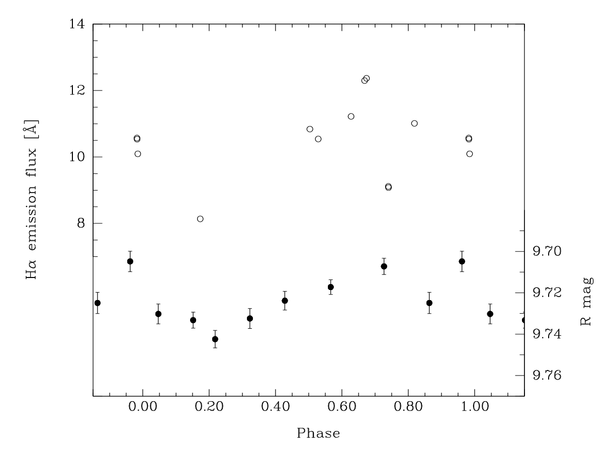
A very asymmetrical shape of the -band light curve, with a deeper minimum at phases 0.15–0.30 and large scatter at the phase 0.85 is probably related to a specific wavelength range covered by this band, which includes the H emission line. As we showed in our previous work, this line is doubled-peaked and strongly variable (see e.g. Fig. 1 in Hubrig et al. 2010 (2010)). The radial velocity of the blue component changes from 33.6 to 67.5 km s-1 whereas the red component, which actually appears triple in the phase 0.17, is shifted by 25.5 to 119.6 km s-1. Our measurements of the H emission line flux over the rotation cycle on available HARPS and UVES spectra presented in Fig. 3 do not contradict this proposition. However, the secondary minimum in the emission flux appears at phase 0.74. The phases of the minima in the measured values roughly coincide with the phases where the longitudinal field approaches zero value, i.e. close to the magnetic equator.
| MJD | Phase | ||||
|---|---|---|---|---|---|
| [G] | [G] | ||||
| 54609.190 | 0.060 | 312 | 32 | 454 | 42 |
| 54610.081 | 0.081 | 235 | 28 | 317 | 35 |
| 55285.141 | 0.125 | 132 | 54 | 149 | 68 |
| 55286.115 | 0.148 | 25 | 48 | 209 | 74 |
| 55287.107 | 0.172 | 49 | 36 | 96 | 61 |
| 55311.142 | 0.743 | 202 | 44 | 235 | 56 |
| 55312.068 | 0.765 | 206 | 48 | 241 | 60 |
| 55320.056 | 0.955 | 526 | 46 | 784 | 57 |
| 55322.149 | 0.004 | 360 | 50 | 568 | 74 |
| 55323.224 | 0.030 | 393 | 51 | 515 | 75 |
| 55324.073 | 0.050 | 359 | 63 | 453 | 64 |
| 55327.159 | 0.124 | 25 | 49 | 44 | 59 |
| 55334.071 | 0.288 | 238 | 57 | 338 | 66 |
| 55335.152 | 0.314 | 351 | 75 | 389 | 84 |
| 55348.097 | 0.621 | 168 | 44 | 322 | 60 |

The logbook of the FORS 2 spectropolarimetric observations is presented in Table 1. In the first column we show the MJD values for the middle of each spectropolarimetric observation. The phases of measurements of the magnetic field are listed in Column 2. In Columns 3 and 4 we present the longitudinal magnetic field using the whole spectrum and the longitudinal magnetic field using only the hydrogen lines. In the first two lines of the table we list the earlier measurements published by Hubrig et al. (2009 (2009)). The corresponding phase diagram for all available mean longitudinal magnetic field measurements using the whole spectrum and for those using only the hydrogen lines, including the best sinusoidal fit, is shown in Fig. 4. The variation has a mean of G and an amplitude of G.

In Fig. 5 we present the variations of equivalent width, radial velocity, line width, and line asymmetry of a sample of iron lines, the mean magnetic field modulus, and the mean longitudinal magnetic field as a function of the rotational phase. Due to imperfect phase coverage the interpretation of the observed variations of the iron line profiles is not straightforward, but it seems that equivalent width and line asymmetry minima appear in the phase close to the surface field maximum of 3.5 kG and the positive extremum of the longitudinal field, while the presence of a secondary minimum is likely at the phase of the negative extremum of the longitudinal field. The line width is the largest at the phase close to the field positive extremum. The radial velocity variations are most difficult to interpret: it is possible that they show double modulation, but it is not well-resolved in our measurements due to insufficient phase coverage.
3 Discussion
HD 101412 exhibits a single-wave variation of the longitudinal magnetic field during the stellar rotation cycle. These observations are usually considered as evidence for a dominant dipolar contribution to the magnetic field topology. Our recent study of the abundances of HD 101412 using UVES and HARPS spectra resulted in km s-1 (Cowley et al. 2010 (2010)). The inclination angles of disks of Herbig Ae/Be stars (which are expected to be identical with the inclination angle of the stellar rotation axis) can be reliably derived only for resolved observations of disks. Fedele et al. (2008 (2008)) used VLTI/MIDI observations to determine =807∘. Using this value we obtain =31 km s-1. Assuming that HD 101412 is an oblique dipole rotator, we follow the definition of Preston (1967 (1967)):
| (3) |
so that the obliquity angle is given by
| (4) |
From the phase curve determined above, with =47432 G and =45632 G, we find =0.9620.075, which for =807∘ leads to a magnetic obliquity of =8413∘.
We note, however, that there are some gaps in the phase coverage for the mean longitudinal magnetic field observations, especially the extrema of the variation curve are not very well constrained. The true magnetic field geometry can probably be resolved once additional longitudinal magnetic field measurements as well as magnetic field modulus measurements over the full stellar rotation cycle become available in future observations.
For the first time rotation modulated longitudinal magnetic field measurements and photometric observations were used to determine the rotation period in a Herbig Ae star. The detection of a large-scale organised predominately dipolar magnetic field on the surface of the young Herbig Ae star HD 101412 confirms the scenario that the accretion phenomenon in young stellar objects is magnetospheric accretion. However, we are still at the very beginning of learning how magnetic fields of Herbig Ae stars can be incorporated in the modeling of stellar magnetospheres which takes into account the full complexity of the circumstellar environment, including the observed outflows and jets in these objects.
Longitudinal magnetic fields of the order of a few hundred Gauss have been detected in about a dozen Herbig Ae stars (e.g., Hubrig et al. 2004c (), 2006 (2006), 2007 (2007), 2009 (2009); Wade et al. 2007 (2007); Catala et al. 2007 (2007)). For the majority of these stars rather small fields were measured, of the order of only 100 G or less. Due to the presence of the rather strong magnetic field in the atmosphere of HD 101412, and a very low value of 3 km s-1, this star is one of the most suitable targets to study its environment, which includes the magnetosphere, the accretion disk, and the disk wind, altogether producing prominent emission features in the hydrogen line profiles.
Acknowledgements.
We acknowledge the support by grants GAAV IAA301630901 and GAČR 205/08/0003.References
- (1) Burd, A., Cwiok, M., Czyrkowski, H., Dabrowski, R., Dominik, W. et al. 2005, New Astronomy 10, 409
- (2) Catala, C., Alecian, E., Donati, J.-F., et al. 2007, A&A, 462, 293
- (3) Cowley, C. R., Hubrig, S., González, J. F., Savanov, I. 2010, A&A, accepted, also: arXiv:1008.1601
- (4) Fedele, D., van den Ancker, M. E., Acke, B., et al. 2008, A&A, 491, 809
- (5) Hubrig, S., Kurtz, D. W., Bagnulo, S., et al. 2004a, A&A, 415, 661
- (6) Hubrig, S., Szeifert, T., Schöller, M., et al. 2004b, A&A, 415, 685
- (7) Hubrig, S., Schöller, M., Yudin, R. V. 2004c, A&A, 428, L1
- (8) Hubrig, S., Yudin, R. V., Schöller, M., Pogodin, M. A. 2006, A&A, 446, 1089
- (9) Hubrig, S., Pogodin, M. A., Yudin, R. V., et al. 2007, A&A, 463, 1039
- (10) Hubrig, S., Stelzer, B., Schöller, M., et al. 2009, A&A, 502, 283
- (11) Hubrig, S., Schöller, M., Savanov, I., et al. 2010, AN, 331, 361
- (12) Kupka, F., Piskunov, N., Ryabchikova, T. A., et al. 1999, A&AS, 138, 119
- (13) Malek, K., Batsch, T., Czyrkowski, H., Cwiok, M., Dabrowski, R. 2010, Advances in Astronomy, Vol. 2010, Article ID 194946
- (14) Mikulášek et al. 2010, in preparation
- (15) Muzerolle, J., D’Alessio, P., Calvet, N., Hartmann, L. 2004, ApJ, 617, 406
- (16) Piskunov, N. E. 1999, in “Solar polarization”, Nagendra K. N., Stenflo J. O., eds., Astrophys. Space Sci. Library Vol. 243, Kluwer Academic Publishers, Dordrecht, p. 515
- (17) Pojmański, G. 2002, Acta Astron., 52, 397
- (18) Press, W. H., Teukolsky, S. A., Vetterling, W. T., Flannery, B. P. 1992, Numerical Recipes, 2nd ed. (Cambridge University Press: Cambridge)
- (19) Preston, G. W. 1967, ApJ, 150, 547
- (20) Ruczinski, S. M., Zwintz, K., Hareter, M., Pojmański, G., Kuschnig, R. et al. 2010, arXiv:1008.4599
- (21) Seber, G. A. F. 1977, Linear Regression Analysis (Wiley: New York)
- (22) Wade, G. A., Bagnulo, S., Drouin, D., et al. 2007, MNRAS, 376, 1145
4 Appendix A: The search for periodic variations
The continuously updated archive of the All Sky Automated Survey (ASAS) is a useful source of photometric observations. Observations were obtained from two ASAS observing stations, one in LCO, Chile (since 1997) and the other on Haleakala, Maui (since 2006). Both are equipped with two wide-field instruments, observing simultaneously in and band. More details and the data archive are on http://www.astrouw.edu.pl/asas/. After removing observations of declared low quality (C, D) and apparent outliers, we obtained a set of 539 -band and 920 -band measurements well covering the periods 1997–1999 and 2000–2009, respectively. The robotic telescope Pi of the Sky has been designed to monitor a significant fraction of the sky with good time resolution. The final detector consists of two sets of 16 cameras, one camera covering a field of view of 20. The set of the HD 101412 measurements covers the time interval of 2006–2009. More details can be found at http://grb.fuw.edu.pl/. CCD photometry was done without any filter, so that the results are similar to a broad-band colour. The star was also observed over eight nights in 2010 April employing the 0.5 m reflector with the classical photometer in SAAO in , using a fairly conventional single channel photometer with a Hamamatsu R943–02 GaAs tube. We obtained 78 triads of measurements with an inner accuracy of 9.4, 6.4, and 6.6 mmag, respectively.
The very good initial estimate of the period allows us to describe the observed periodic variations by a series of phenomenological models described by a minimum number of free parameters, including the period and the origin of epoch counting . The behaviour of the light curves in and is nearly the same. For simplicity we assumed a similar behaviour also for light curves in and bands, while the light curve behaves differently. The periodic component in light variations can then be described by means of periodic functions and :
| (5) | |||
| (6) |
The functions and are the simplest normalised periodic function that represent the observed photometric variations in detail. The phase of the brightness extreme is defined to be 0.0, and the effective amplitude is defined to be 1.0. The functions, being the sum of three terms, are described by two dimensionless parameters and . and are the phase function. Assuming linear ephemeris, we respectively obtain:
| (7) |
where is the phase shift of the basic minimum of the function versus zero phase.
Periodic changes of magnitudes in : and changes in : are given by the relations:
| (8) |
where is the semiamplitude of light changes common to all bands and is the amplitude of an additional component of light variability being non-zero only in . and are mean magnitudes in the individual bands.
The periodic variations of the mean value of the longitudinal component of the magnetic field intensity derived from all lines can be well approximated by the simple cosinusoid:
| (9) |
where is the mean magnetic field intensity, is the semiamplitude of the variations, and is the phase of the magnetic field minimum.
All 18 model parameters were computed simultaneously by a weighted non-linear least-square method regression applied to the complete observational material representing in total 3134 individual measurements. We found the refined value of the rotational period and the origin of phase counting put at the light maximum .
| (10) |
Parameters describing the functions and are: , , , and , the function primary minimum phase , the phase of the secondary minimum , the semiamplitude of light changes mmag, the semiamplitude mmag, mag, mag, and mag. The phase of the minimum of the mean projected intensity of the magnetic field , , the mean value of it: G, and the semiamplitude G.
5 Appendix B: Non-periodic variations
Relatively precise ASAS and data show an apparent evolution of the mean values to the extent of several hundredths of a magnitude over time scales of several years (see Fig. 6). For this reason, we use detrended magnitudes, i.e. magnitudes where we have removed the long term trends, in our search of periodic stellar variability.

An inspection of the light variation in plotted over the rotational phase in 2006–2009 reveals dramatic seasonal variations in the shape of the light curve. Unfortunately, the low accuracy of the photometric measurements together with the observed long-term instability and the large stochastic changes do not allow us to analyse this phenomenon more deeply. Using principal component analysis tools, we tested the possibility of seasonal changes in the shape of the light curve in the first decade of this century. We conclude that the light curve as defined by ASAS and SAAO measurements was quite stable during this period.
Herbig Ae/Be stars are known to vary in a complex way. The mechanism causing this variability is not well understood. These more or less stochastic variations amount up to several hundreds of a magnitude on time scales from several minutes to tens of years (see e.g. Ruczinski et al. 2010 (2010)). The light changes of HD 101412 in and presented in Fig. 6 can be treated as stochastic variations on the scale of tens of years. Nevertheless, there is also evidence of such changes on much shorter time-scales.
Our own 78 photoelectric measurements in 2010 April in SAAO were obtained in a total of 12 sets over eight nights. The duration of one measurement set was not longer than 15 minutes and we assumed that the brightness of the star did not change during the exposure. Then we can relatively well estimate the typical inner uncertainty of one individual measurement as 9.4, 6.4, and 6.6 mmag in , and , respectively. However, the means in particular sets in , , and , consisting of six individual measurements in the average, show an additional scatter of 14, 10, and 11 mmag (see Fig. 7). We inferred that this scatter is due to stochastic changes on the scale of hours or tens of hours. It should be noted that the observed stochastic variations in particular colours are highly correlated, whereas their amplitude is the largest in the -band. Such a behaviour is certainly somehow related to the physics of the mechanisms causing such changes.
Because of the circumstance that we do not have at our disposal measurements in and during one night, we estimate the inner accuracy of these measurements implicitly. The mean scatter of detrended ASAS data in and are 16 and 10 mmag. Assuming that the estimate of stochastic noise in of 11 mmag is valid or smaller for all ASAS measurements, we conclude, that the inner uncertainty of one ASAS observation is smaller than 12 mmag. The ASAS estimates of uncertainty of observations should then be smaller by a factor of 0.6 compared to observations. The inner accuracy should then be about 7 mmag, as well as the measure of the stochastic scatter. In all cases the stochastic scatter in is not allowed to be larger than 10 mmag. It means that the tendency of the decrease of the stochastic scatter with the increase of the wavelength is supported also by ASAS data. A different amount of stochastic variation is expected in band, where an additional variability mechanism is probably active. The mean scatter in the -band is about 56 mmag. The inner uncertainty of Pi measurements can be derived from magnitudes obtained in individual nights – it is estimated to be 49 mmag. The stochastic scatter then can be evaluated as 30 mmag.
