Non-differentiable Bohmian trajectories

Quantum mechanis often is praised as a theory which unifies classical mechanics and classical wave theory. Quanta are said to behave either as particles or waves, depending on the type of experiment they are subjected. But where in the standard formalism can the particles of the interpretive talk be found? Perhaps only to some degree in the reduction postulate applied to position measurements. In reaction to this unsatisfactory state of affairs, Bohmian mechanics introduces a mathematically precise particle concept into quantum mechanical theory. The fuzzy wave functions are supplemented by sharp particle world lines. Through this additional structure some quantum phenoma like the double slit experiment have lost their mystery.

Clearly the additional structure of particle world lines brings along its own mathematical problems. Ordinary differential equations are generated from solutions of partial differential equations. A mathematically convincing general treatment so far has been given for a certain type of wave functions which do not exhaust all possible quantum mechanical situations. Exactly this fact has led some workers to doubt that a Bohmian mechanics exists for all initial states $\Psi_{0}$ of a Schrödinger evolution $t\mapsto e^{-iht}\Psi_{0}.$ We shall show on one specific case of a counter example $\Psi_{0}$ how the problem might be resolved in general. We approximate the state $\Psi_{0},$ for which the Bohmian velocity field does not exist, by states which do have one. Their integral curves turn out to converge to limit curves which can be taken to constitute the Bohmian mechanics of the state unamenable to Bohmian mechanics on first sight.

Let $\psi:\mathbb{R}\times\mathbb{R}^{s}\rightarrow\mathbb{C}$ be twice continuously differentiable, i.e. $\psi\in C^{2}\left(\mathbb{R}\times\mathbb{R}^{s}\right),$ and let $\psi$ obey Schrödinger’s partial differential equation

with $V:\mathbb{R}^{s}\rightarrow\mathbb{R}$ being smooth, i.e., $V\in C^{\infty}\left(\mathbb{R}^{s}\right).$ From $\psi,$ which is called a classical solution of Schrödinger’s equation, a deterministic time evolution $x\mapsto\gamma_{x}\left(t\right)$ of certain points $x\in\mathbb{R}^{s}$ can be derived: If there exists a unique maximal solution $\gamma_{x}:I_{x}\rightarrow\mathbb{R}^{s}$ to the implicit first order system of ordinary differential equations

with the initial condition $\gamma\left(0\right)=x,$ one takes $\gamma_{x}$ as the evolution of $x.$ Here $\rho_{\psi}:\mathbb{R}\times\mathbb{R}^{s}\rightarrow\mathbb{R}$ and $j_{\psi}:\mathbb{R}\times\mathbb{R}^{s}\rightarrow\mathbb{R}^{s}$ with

obey the continuity equation $\partial_{t}\rho_{\psi}\left(t,x\right)=-$div$j_{\psi}\left(t,x\right)$ for all $\left(t,x\right)\in\mathbb{R}\times\mathbb{R}^{s}.$ From now on we shall drop the index $\psi$ from $\rho_{\psi}$ and $j_{\psi}.$

For certain solutions¹¹ 1 The simplest explicitly solvable example is provided by the plane wave solution $\psi\left(t,x\right)=e^{-i\left|k\right|^{2}t+ik\cdot x}.$ Its Bohmian evolution $\Phi$ obeys $\Phi\left(t,x\right)=tk.$ Another explicitly solveable case is given by a Gaussian free wave packet. $\psi$ the curves $\gamma_{x}$ can be shown to exist on a maximal domain $I_{x}=\mathbb{R}$ for all $x\in\mathbb{R}^{s}:$ If $\psi$ has no zeros, then the velocity field $v=j/\rho$ is a $C^{1}$-vector field. $v$ then obeys a local Lipschitz condition such that the maximal solutions are unique. If in addition there exist continuous nonnegative real functions $\alpha,\beta$ with $\left|v\left(t,x\right)\right|\leq\alpha\left(t\right)\left|x\right|+\beta\left(t\right)$ then all maximal solutions equation (2) are defined on $\mathbb{R}$ and the general solution

extends to all of $\mathbb{R}\times\mathbb{R}^{s}.$ (Thm 2.5.6, ref. [1]) Due to the uniqueness of maximal solutions the map $\Phi\left(t,\cdot\right):\mathbb{R}^{s}\rightarrow\mathbb{R}^{s}$ is a bijection for all $t\in\mathbb{R}.$ It obeys²² 2 Here $\Phi\left(t,\Omega\right)=\left\{\Phi\left(t,x\right)\left|x\in\Omega\right.\right\}.$

for all $t\in\mathbb{R}$ and for all open subsets $\Omega\subset\mathbb{R}^{s}$ with sufficiently smooth boundary such that the integral theorem of Gauss can be applied to the space time vector field $\left(\rho,j\right)$ on the domain $\bigcup\nolimits_{t^{\prime}\in\left(0,t\right)}\Phi\left(t^{\prime},\Omega\right).$ [2]

These undisputed mathematical facts have instigated Bohm’s amendment of equation (1) in order to explain the fact that macroscopic bodies usually are localized much stricter than their wave functions suggest.

In Bohm’s completion of nonrelativistic quantum mechanics it is assumed that any closed system has at any time, in addition to its wave function, a position in its configuration space and that this position evolves according to the general solution $\Phi$ induced by the wave function. One says that the position is guided by $\psi$ since $\Phi$ is completely determined by $\psi$ (and no other forces than the ones induced by $\psi$ are allowed to act on the position). More specifically, $\gamma_{x}$ is assumed to give the position evolution for an isolated particle with wave function $\psi\left(0,\cdot\right)$ and position $x$ – both at time $t=0.$

As is common in standard quatum mechanics, $\psi\left(0,\cdot\right)$ is supposed to obey

The nonnegative density $\rho\left(0,\cdot\right)$ is interpreted as the probability density of the position which the particle has at time $t=0.$ Since an initial position $x$ is assumed to evolve into $\gamma_{x}\left(t\right),$ the position probability density at time $t$ is then, due to equation (4), given by $\rho\left(t,\cdot\right).$ In particular, Bohm’s completion gives the position probabilities among all the other spectral probability measures a fundamental status, since the empirical meaning of the other ones, as for instance momentum probabilities, all are deduced from position probabilities.

There are classical solutions of Schrödinger’s equation, whose general solution $\Phi$ does not extend to all of $\mathbb{R}\times\mathbb{R}^{s}.$ An obstruction to do so can be posed by the zeros of $\psi.$ In the neigbourhood of such zero the velocity field $v=j/\rho$ may be unbounded and $v$ then lacks a continuous extension into the zero. As an example consider a time $0$ wave function $\psi\left(0,\cdot\right):\mathbb{R}^{2}\rightarrow\mathbb{C},$ for which $\psi\left(0,x,y\right)=x^{2}+iy^{2}$ within a neighbourhood $U$ of its zero $\left(x,y\right)=\left(0,0\right).$ Within $U$ for the velocity field follows

Hence for $0<\left|\phi\right|<\pi/2$ we have $v^{1}\left(r\cos\phi,r\sin\phi\right)\rightarrow-\infty$ for $r\rightarrow 0$ with $\phi$ fixed. Thus the implicit Bohmian evolution equation (2) is singular in a zero of the wave function whenever the velocity field does not have a continuous extension into it. As a consequence the evolution $\gamma_{x}$ of such a zero $x$ is not defined by equation (2).

As a related phenomenon there are solutions to equation (2) which begin or end at a finite time because they terminate at a zero of $\psi.$ A nice example [3] for this to happen provide the zeros of the harmonic oscillator wave function $\psi:\mathbb{R}^{2}\rightarrow\mathbb{C}$ with

E.g., the points $\left|x\right|=1$ are zeros of $\psi\left(t,\cdot\right)$ at the times $t\in\pi\mathbb{Z}.$ They are singularities of $v$ since

Note however that $\Im\frac{\partial_{x}\psi\left(0,x\right)}{\psi\left(0,x\right)}=0$ for $x\neq\pm 1.$

There are more challenges to Bohmian mechanics. The notion of distributional solutions to a partial differential equation like (1) raises the question whether these solutions support a kind of Bohmian particle motion like the classical solutions do. After all quantum mechanics employs such distributional solutions.

In standard quantum mechanics the classical solutions, i.e. the $C^{2}$-solutions of equation (1), do not represent all physically possible situations. Rather a more general quantum mechanical evolution is abstracted from equation (1). It is given by the socalled weak solutions

with $\hbar h$ being a self-adjoint, ususally unbounded hamiltonian corresponding to equation (1). The domain $D_{h}$ of $h$ does not comprise all of $L^{2}\left(\mathbb{R}^{s}\right),$ yet it is dense in $L^{2}\left(\mathbb{R}^{s}\right).$ Since $h$ is self-adjoint, the exponential $e^{-iht}$ has a unique continuous extension to $L^{2}\left(\mathbb{R}^{s}\right).$ This unitary evolution operator $e^{-iht}$ stabilizes the domain of $h$ as a dense subspace of $L^{2}\left(\mathbb{R}^{s}\right).$ Thus if and only if an initial vector $\Psi_{0}$ belongs to $D_{h},$ equation (1) generalizes to

for all $t\in\mathbb{R}.$ For $\Psi_{0}\notin D_{h}$ equation (5) does not hold for any time.

Yet the construction of Bohmian trajectories needs much more than the evolution $\Psi_{0}\mapsto\Psi_{t}$ within $L^{2}\left(\mathbb{R}^{s}\right),$ since the elements of $L^{2}\left(\mathbb{R}^{s}\right)$ are equivalence classes $\left[f\right]$ of functions $f\in\mathcal{L}^{2}\left(\mathbb{R}^{s}\right).$ It rather needs a trajectory of functions instead of a trajectory of equivalence classes of square-integrable functions. If there exists a function $\psi\in C^{1}\left(\mathbb{R}\times\mathbb{R}^{s}\right)$ such that $\Psi\left(t,\cdot\right)=\left[\psi\left(t,\cdot\right)\right]$ holds for all $t\in\mathbb{R},$ then $\psi$ is unique and the Bohmian equation of motion (2) can be derived from the evolution $\Psi_{0}\mapsto\Psi_{t}$ through $\psi.$ When does there exist such $\psi?$

Due to Kato’s theorem (e.g. Thm X.15 of ref. [4]) the Schrödinger hamiltonians $h,$ corresponding to potentials $V$ from a much wider class than just $C^{\infty}\left(\mathbb{R}^{s}:\mathbb{R}\right),$ have the same domain as the free hamiltonian $-\Delta,$ namely the Sobolev space $W^{2}\left(\mathbb{R}^{s}\right).$ This is the space of all those $\Psi\in L^{2}\left(\mathbb{R}^{s}\right)$ which have all of their distributional partial derivatives up to second order being regular distributions belonging to $L^{2}\left(\mathbb{R}^{s}\right).$ Since $D_{h}$ is stabilized by the evolution $e^{-iht},$ for any $\Psi_{0}\in D_{h}$ there exists for any $t\in\mathbb{R}$ a function $\psi\left(t,\cdot\right)\in\mathcal{W}^{2}\left(\mathbb{R}^{s}\right)$ such that

However, for this family of time parametrized functions $\psi\left(t,\cdot\right)$ the Bohmian equation of motion in general does not make sense since $\psi\left(t,\cdot\right)$ need not be differentiable in the classical sense.³³ 3 Only for $s=1$ Sobolev’s lemma (Thm IX.24 in Vol 2 of ref. [4]) says that $\left[\psi\left(t,\cdot\right)\right]$ has a $C^{1}$ representative within $\mathcal{L}^{2}\left(\mathbb{R}\right).$ From such a $C^{1}$ representative $\psi\left(t,\cdot\right)$ the current $j$ follows as a continuous vector field and a continuous velocity field $v$ can be derived outside the zeros of $\psi.$ However, $v$ does not need to obey the local Lipschitz condition implying the local uniquenss of its integral curves.

Therefore some stronger restriction of initial data than $\Psi_{0}\in D_{h}$ is needed in order to supply the state evolution $\Psi_{0}\mapsto e^{-iht}\Psi_{0}$ with Bohm’s amendment. For a restricted set of initial states $\left(x,\Psi_{0}\right)$ and for a fairly large class of static potentials a Bohmian evolution has indeed been constructed in [5] and [6]. There it is shown that for any $\Psi_{0}\in\bigcap\nolimits_{n\in\mathbb{N}}D_{h^{n}}=:C_{h}^{\infty}$ there exists

• •

  a (time independent) subset $\Omega\subset\mathbb{R}^{s}$

• •

  for any $t$ a square-integrable function $\psi\left(t,\cdot\right)$

such that the restriction of $\psi\left(t,\cdot\right)$ to $\Omega$ belongs to $C^{\infty}\left(\Omega\right)$ and equation (6) holds. The set $\Omega$ is obtained by removing from $\mathbb{R}^{s}$ first the points where the potential function $V$ is not $C^{\infty},$ second the zeros of $\psi\left(0,\cdot\right),$ and third those points $x$ for which the maximal solution $\gamma_{x}$ does not have all of $\mathbb{R}$ as its domain. Surprizingly, $\Omega$ is still sufficiently large, since

On this reduced set $\Omega$ of initial conditions a Bohmian evolution $\Phi:\mathbb{R}\times\Omega\rightarrow\mathbb{R}^{s}$ can be constructed. Thus if $\Psi_{0}\in C_{h}^{\infty}$ and if the initial position $x$ is distributed within $\mathbb{R}^{s}$ with probability density $\left|\psi\left(0,\cdot\right)\right|^{2}$ then the global Bohmian evolution $\gamma_{x}$ of $x$ exists with probability $1.$

How about initial conditions $\Psi_{0}\in L^{2}\left(\mathbb{R}^{s}\right)\smallsetminus C_{h}^{\infty}?$ Can the equation of motion (2) still be associated with $\Psi_{0}?$ Hall has devised a specific counterexample $\Psi_{0}\notin D_{h}$ which leads to a wave function $\psi$ which at certain times is nowhere differentiable with respect to $x$ and thus renders impossible the formation of the velocity field $v.$ Therefore it has been brought forward that the Bohmian amendment of standard quantum mechanics is “formally incomplete” and it has been claimed that the problem is unlikely to be resolved. [7]

A promising way to tackle the problem is to succesively approximate the initial condition $\Psi_{0}\notin D_{h}$ by a strongly convergent sequence of vectors $\left(\Psi_{0}^{n}\right)\in C_{h}^{\infty}.$ For each of the vectors $\Psi_{0}^{n}$ a Bohmian evolution $\Phi_{n}$ exists. We do not know whether it has actually been either disproven or proven that the sequence of evolutions does converge to a limit $\Phi$ and that the limit depends on the chosen sequence $\Psi_{0}^{n}\rightarrow\Psi_{0}.$

Here we shall explore this question within the simplified setting of a spatially one dimensional example. We will make use of an equation for $\gamma_{x}$ which has already been pointed out in [5] and which does not rely on the differentiability of $j.$ In this case equation (4) can be generalized in order to determine a nondifferentiable Bohmian trajectory $\gamma_{x}$ by choosing $\Omega=\left(-\infty,x\right)$ in (4) as follows.

Consider first the case of a $C^{2}$-solution of equation (1) generating a general solution $\Phi:\mathbb{R}\times\mathbb{R}\rightarrow\mathbb{R}$ of the Bohmian equation of motion (2). Since because of their uniqueness the maximal solutions do not intersect, we have $\Phi\left(t,\left(-\infty,x\right)\right)=\left(-\infty,\Phi\left(t,x\right)\right)=\left(-\infty,\gamma_{x}\left(t\right)\right).$ From this it follows by means of equation (4) that

As a check we may take the derivative of equation (7) with respect to $t.$ This yields

Making use of local probability conservation $\partial_{t}\rho=-\partial_{x}j$ we recover by partial integration equation (2).

Now observe that the equation (7) for $\gamma_{x}\left(t\right)$ is meaningful not only when $\psi$ is a square integrable $C^{2}$-solution of equation (1) but also if $\psi\left(t,\cdot\right)$ is an arbitrary representative of $\Psi_{t}$ with arbitrary $\Psi_{0}\in L^{2}\left(\mathbb{R}\right).$ In order to make this explicit let $E_{x}:L^{2}\left(\mathbb{R}\right)\rightarrow L^{2}\left(\mathbb{R}\right)$ with $x\in\mathbb{R}$ denote the spectral family of the position operator. For the orthogonal projection $E_{x}$ holds

The expectation value $\left\langle\Psi,E_{x}\Psi\right\rangle$ of $E_{x}$ with a unit vector $\Psi\in L^{2}\left(\mathbb{R}\right)$ thus yields the cumulative distribution function of the position probability given by $\Psi.$ If we define $F:\mathbb{R}^{2}\rightarrow\left[0,1\right]$ through $F\left(t,x\right)=\left\langle\Psi_{t},E_{x}\Psi_{t}\right\rangle,$ then equation (7) is equivalent to

Thus, the graph $\left\{\left(t,\gamma_{x}\left(t\right)\right)\left|t\in\mathbb{R}\right.\right\}$ of a trajectory is a subset of the level set of $F$ which contains the point $\left(0,x\right).$ If $\Psi_{n}$ is a sequence in $L^{2}\left(\mathbb{R}^{s}\right)$ which converges to $\Psi$ then

because $e^{-iht},E_{x},$ and $\left\|\cdot\right\|^{2}$ are continuous mappings.

Note that for any $t\in\mathbb{R}\$the function $F\left(t,\cdot\right):\mathbb{R}\rightarrow\left[0,1\right]$ is continuous and monotonically increasing. Furthermore $\lim_{x\rightarrow-\infty}F\left(t,x\right)=0$ and $\lim_{x\rightarrow\infty}F\left(t,x\right)=1.$ The monotonicity is a strict one if $\psi\left(t,\cdot\right)$ does not vanish on any interval. Thus for any $\left(t,x\right)\in\mathbb{R}^{2}$ there exists at least one $\gamma_{x}\left(t\right)\in\mathbb{R}$ such that equation (8) holds. (For those values $t$ for which $F\left(t,\cdot\right)$ is strictly increasing, there exists exactly one $\gamma_{x}\left(t\right)\in\mathbb{R}$ such that equation (8) holds.) The function $F$ cannot be constant in an open neighbourhood of some point $\left(t,x\right)$ if the hamiltonian is bounded from below. Thus for any $x\in\mathbb{R},$ for which there does not exist a neighbourhood on which $F\left(0,\cdot\right)$ is constant, we now define $\gamma_{x}:\mathbb{R}\rightarrow\mathbb{R}$ to be the unique continuous mapping for which

Note that $\gamma_{x}:\mathbb{R}\rightarrow\mathbb{R}$ is continuous, yet need not be differentiable.

Let us now illustrate this construction of not necessarily differentiable Bohmian trajectories by means of a solution $t\mapsto\Psi_{t}\notin D_{h}$ of the Schrödinger equation (5) describing a particle confined to a finite interval on which the potential $V$ vanishes. This solution has been used by Hall [7] as a counter example to Bohmian mechanics. Similar ones have been used in order to illustrate an “irregular” decay law $t\mapsto\left|\left\langle\Psi_{0},\Psi_{t}\right\rangle\right|^{2}.$ [8] Both works have made extensive use of Berry’s earlier results concerning this type of wave functions. [9]

The (reduced) classical Schrödinger equation corresponding to the quantum dynamics is

for all $\left(t,x\right)\in\mathbb{R}\times\left[0,\pi\right]$ together with the homogeneous Dirichlet boundary condition $\psi\left(t,0\right)=\psi\left(t,\pi\right)=0$ for all $t\in\mathbb{R}.$ The corresponding hamiltonian’s domain $D_{h}$ is the set of all those $\Psi\in L^{2}\left(0,\pi\right)$ which have an absolutely continuous representative $\psi$ vanishing at $0$ and $\pi$ and whose distributional derivatives up to second order belong to $L^{2}\left(0,\pi\right).$ As an initial condition we choose the equivalence class of the function

Since within the class $\Psi_{0}=\left[\psi\left(0,\cdot\right)\right]$ there does not exist an absolutely continuous function vanishing at $0$ and $\pi$ the equivalence class $\Psi_{0}$ does not belong to $D_{h}.$ As a consequence for any $t$ the vector $\Psi_{t}=e^{-iht}\Psi_{0}$ does not belong to $D_{h}.$ This in turn implies that $\Psi_{t}$ does not have a representative within the class of $C^{2}$-functions on $\left[0,\pi\right]$ with vanishing boundary values.

The hamiltonian $h$ is self-adjoint. An orthonormal basis formed by eigenvectors of $h$ is represented by the functions $u_{k}$ with

For $n\in\mathbb{N}$ the $C^{\infty}$-function $\psi_{n}:\mathbb{R}^{2}\rightarrow\mathbb{C}$ with

is a classical solution to the Schrödinger equation (9) on $\mathbb{R}^{2}$ and fulfills homogeneous Dirichlet boundary conditions at $x=0$ and $x=\pi.$ Furthermore $\psi_{n}$ is periodic not only in $x$ but also in $t$ with period $2\pi.$ More precisely $\psi\left(t,\cdot\right)$ is an odd trigonometric polynomial of degree $2n+1$ for any $t\in\mathbb{R}.$ In addition $\psi_{n}\left(t,\cdot\right)$ also is even with respect to reflection at $\pi/2,$ i.e., it holds

for all $x\in\mathbb{R}.$ The functions $\psi_{n}\left(\cdot,x\right)$ are trigonometric polynomials of degree $\left(2n+1\right)^{2}.$

As is well known, the sequence $\left(\psi_{n}\left(0,\cdot\right)\right)_{n\in\mathbb{N}}$ converges pointwise on $\mathbb{R}.$ Its limit is the odd, piecewise constant $2\pi$-periodic function $\sigma\left(0,\cdot\right)$ with

$\sigma\left(0,\cdot\right)$ is discontinuous at $x\in\pi\cdot\mathbb{Z}.$ For any $t\in\mathbb{R}$ the sequence $\left(\psi_{n}\left(t,\cdot\right)\right)_{n\in\mathbb{N}}$ converges pointwise on $\mathbb{R}$ to a function $\psi\left(t,\cdot\right).$ For rational $t/\pi$ this function is piecewise constant. [9] However for irrational $t/\pi$ the real- and imaginary parts of $\psi\left(t,\cdot\right)$ restricted to any open real interval have a graph with noninteger dimension. [9] Thus for irrational $t/\pi$ the function $\psi\left(t,\cdot\right)$ is non-differentiable on any real interval. As an illustration we give in Figure 1 the graph of

for $0<x<1/2$ together with the partial sum over $k\in\left\{501,\ldots 750\right\}$ visible as the small noisy signal along the abscissa

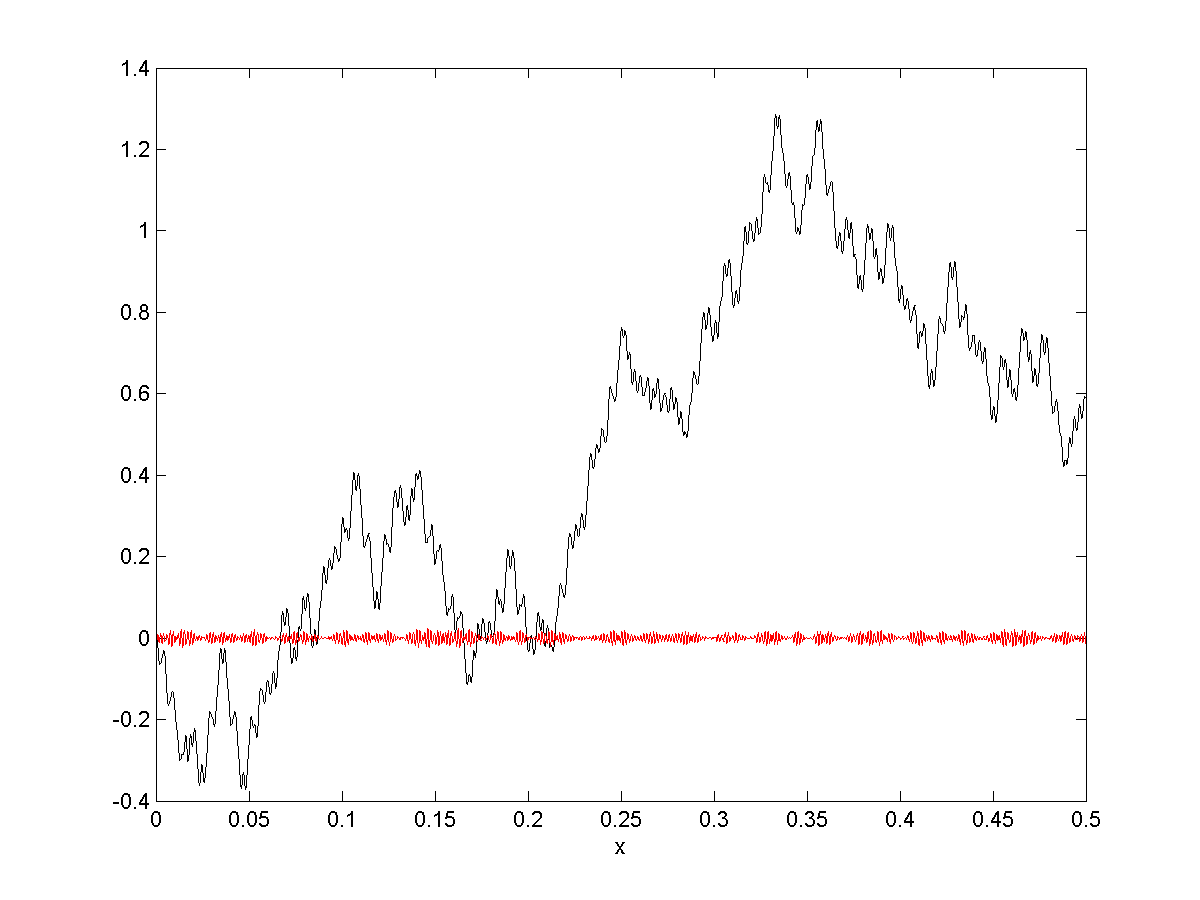
Similarly, for given $x\in\left(0,\pi\right)$ the mapping $t\mapsto\psi\left(t,x\right)$ does not belong to the set of piecewise $C^{1}$-functions on $\left[0,2\pi\right].$ This can be seen as follows. First note that for given $x$ the $2\pi$-periodic function $\psi\left(\cdot,x\right)$ has the Fourier expansion

Assume now that $\psi\left(\cdot,x\right)$ is piecewise $C^{1}.$ Then, according to a well known property of Fourier coefficients, there exists a positive real constant $C$ such that $n\left|c_{n}\right|<C$ for all $n\in\mathbb{N}.$ This implies that

with the positive constant $C^{\prime}=\pi\sqrt{\pi}C/4.$ However, for $x\notin\pi\cdot\mathbb{Z}$ there exists some real constant $\varepsilon>0$ such that the set $\left\{k\in\mathbb{N}:\left|\sin\left[\left(2k+1\right)x\right]\right|>\varepsilon\right\}$ contains infinitely many elements. Thus for $x\notin\pi\cdot\mathbb{Z}$ the estimate (11) cannot hold and therefore the function $t\mapsto\psi\left(t,x\right)$ cannot be piecewise $C^{1}$ on $\left[0,\pi\right].$

In Figure 2 we plot the time dependence

for $0<t<1/2$ together with the partial sum

(noisy signal along abscissa).

The restriction of the limit $\sigma\left(0,\cdot\right)$ to $\left[0,\pi\right]$ represents the same $L^{2}$ element as $\psi\left(0,\cdot\right)$ does. Thus $\lim_{n\rightarrow\infty}\left\|\left[\widetilde{\psi_{n}}\left(0,\cdot\right)\right]-\Psi_{0}\right\|=0,$ when $\widetilde{\psi_{n}}$ denotes the restriction of $\psi_{n}$ to $\mathbb{R}\times\left[0,\pi\right].$ Correspondingly $\rho_{n}\left(0,\cdot\right)=\left|\psi_{n}\left(0,\cdot\right)\right|^{2}$ converges towards the density of the equipartition on $\left[0,\pi\right].$ Additionally, due to the continuity of the evolution operator $e^{-iht},$ the sequence of equivalence classes $\left[\widetilde{\psi_{n}}\left(t,\cdot\right)\right]\in C_{h}^{\infty}$ approximates the $L^{2}$ vector $\Psi_{t}=e^{-iht}\Psi_{0},$ i.e., for all $t$ holds

Since also $E_{x}:L^{2}\left(\mathbb{R}\right)\rightarrow L^{2}\left(\mathbb{R}\right)$ is continuous, the time dependent cumulative position distribution function $F:\mathbb{R}\times\left[0,\pi\right]\rightarrow\left[0,1\right]$ with $F\left(t,x\right):=\left\langle\Psi_{t},E_{x}\Psi_{t}\right\rangle$ obeys

The level lines of the functions $F_{n}:\mathbb{R}\times\left[0,\pi\right]\rightarrow\left[0,1\right]$ with $F_{n}\left(t,x\right):=\int_{0}^{x}\left|\psi_{n}\left(t,y\right)\right|^{2}dy$ thus converge to the continuous level lines of $F.$

Figure 3 shows some level lines of $F_{n}$ for $n=5,10,20$ starting off at equal positions at $t=0.$ The level lines inherit the period $\pi/4$ of $F\left(\cdot,x\right),$ which has this periode since the frequencies appearing in the even function $\left|\psi_{n}\left(\cdot,x\right)\right|^{2}$ are $0,8,16,\ldots$

Figure 4 shows the case $n=1000.$ Increasing $n$ from $20$ to $1000$ hardly alters the level lines.

References

- [1] B Aulbach, Gewöhnliche Differenzialgleichungen, Elsevier, 2004
- [2] D Dürr, S Teufel, Bohmian mechanics, Springer, Berlin, 2009
- [3] K Berndl, Global existence and uniqueness of Bohmian trajectories, arXiv:quant-ph/9509009, 1995 (published in: Bohmian mechanics and quantum theory: an appraisal, Eds. J T Cushing et al, Kluwer, Dordrecht, 1996)
- [4] M Reed, B Simon, Methods of modern mathematical physics II, Academic press, New York, 1975
- [5] K Berndl et al, On the global existence of Bohmian mechanics, Comm Math Phys 173 (1995) 647 - 673
- [6] S Teufel, R Tumulka, Simple proof of global existence of Bohmian trajectories, Comm Math Phys 258 (2004) 349-65
- [7] M J W Hall, Incompleteness of trajectory-based interpretation of quantum mechanics, Journ Phys A37 (2004) 9549-56
- [8] P Exner, M Fraas, The decay law can have an irregular character, Journ Phys A40 (2007) 1333-40
- [9] M V Berry, Quantum fractals in boxes, Journ Phys A29 (1996) 6617-29