The H Luminosity Function and Star Formation Rate Volume Density at from the NEWFIRM H Survey
Abstract
We present new measurements of the H luminosity function (LF) and star formation rate (SFR) volume density for galaxies at . Our analysis is based on 1.18m narrowband data from the NEWFIRM H (NewH) Survey, a comprehensive program designed to capture deep samples of intermediate redshift emission-line galaxies using narrowband imaging in the near-infrared. The combination of depth ( erg s-1 cm-2 in H at 3) and areal coverage (0.82 deg2) of the 1.18m observations complements other recent H studies at similar redshifts, and enables us to minimize the impact of cosmic variance and place robust constraints on the shape of the LF. The present sample contains 818 NB118 excess objects, 394 of which are selected as H emitters. Optical spectroscopy has been obtained for 62% of the NB118 excess objects. Empirical optical broadband color classification is used to sort the remainder of the sample. A comparison of the LFs constructed for the four individual fields covered by the observations reveals significant cosmic variance, emphasizing that multiple, widely separated observations are required for such analyses. The dust-corrected LF is well described by a Schechter function with erg s-1, Mpc-3, and . We compare our H LF and SFR density to those at , and find a rise in the SFR density , which we attribute to significant evolution. Our H SFR density of yr-1 Mpc-3 is consistent with UV and [O II] measurements at . We discuss how these results compare to other H surveys at , and find that the different methods used to determine survey completeness can lead to inconsistent results. This suggests that future surveys probing fainter luminosities are needed, and more rigorous methods of estimating the completeness should be adopted as standard procedure (for example, with simulations which try to simultaneously reproduce the observed H LF and equivalent width distributions).
Subject headings
galaxies: distances and redshifts – galaxies: evolution – galaxies: luminosity function, mass function – galaxies: photometry – galaxies: star formationI. INTRODUCTION
The luminosity of the H nebular emission line is a star formation rate (SFR) indicator valued for its relatively direct physical connection to short-lived massive stars. In the local universe, it has been well calibrated [23, 26, e.g.,], and extensively used to measure the SFRs of individual galaxies, as well as the SFR density over cosmic volumes [24, 10, 44, 13, 3, 16, 35, 33, 5, 25, 30, e.g.,].
While it is desirable to extend H studies of galaxies to earlier cosmic times, such work is observationally difficult because H is redshifted into the infrared beyond . Early attempts yielded samples of H emitters that were small in size and did not sample representative cosmic volumes, because of the limited depth and areal coverage of the observations [61, 21, 56, e.g.,]. Other SFR indicators, which are accessible in the optical at higher redshift (e.g., the rest-frame UV continuum or other bluer emission lines), have therefore been more commonly used. Measurements of the SFR density have now been made at redshifts as high as . A sharp, order of magnitude decline is seen in the star formation activity of the universe from to the present day [19, see e.g.,]. However, the amalgam of measurements that constitute our current understanding of the cosmic star formation history shows a scatter of at least a factor of a few, which considerably reduces their usefulness as a constraint on models of galaxy evolution.
In this context, it is important to determine the extent to which systematics between different SFR indicators (such as the variable impact of dust attenuation and dependence on metallicity) contribute to the observed scatter in the cosmic star formation history. In particular, it is useful to trace the history with a consistent indicator throughout time, and then compare the overall histories determined with different indicators. This paper represents a step in this process, and aids in the robust extension of H measurements of the SFR density to higher redshift.
Here, we present H luminosity functions (LFs) and SFR densities at . At this redshift, the age of the universe is 6.6 Gyr, assuming a [, , ] = [0.7, 0.3, 1.0] cosmology, which we adopt throughout. Our analysis is based on narrowband (NB) observations from the NEWFIRM H (NewH) Survey (J. C. Lee et al. 2011, in preparation), which has been conducted with the NOAO Extremely Wide-Field Infrared Imager [42, 41, NEWFIRM;] at the KPNO 4 m telescope. The current sample contains 400 H emitting galaxies above 3 significance, which have been identified over an area of 0.82 deg2.
This paper is organized as follows. In Section II, we give an overview of the NewH data that are used in our analysis. In Section III, we describe the selection of NB118 excess emitters. We also discuss the techniques (i.e., dedicated follow-up spectroscopy and empirical broadband color classification) that are used to identify the emission line(s) responsible for the narrowband excess. A description of how we compute emission-line fluxes, luminosities, and equivalent widths (EWs) is provided in Section IV. In Section V, estimates of the survey’s completeness and the surveyed volume are presented, and Section VI presents the H LF and the comoving SFR density at . Comparisons of these results with existing H measurements are described in Section VII. We also compare our results with that of other recent narrowband H surveys, and examine the reasons why inconsistent results may arise between these studies. A discussion of our results and their implications for the evolution of typical galaxies at are provided in Section VIII, and concluding remarks are provided in Section IX. Magnitudes are reported on the AB system [38].
| Field | R.A., Dec | Observation Dates | Filter | Int. Time | FWHM | Limiting Magnitude (AB, 3) | |||
|---|---|---|---|---|---|---|---|---|---|
| (J2000) | (hr) | (arcsec) | SE | SW | NE | NW | |||
| COSMOS | 10:01, +02:01 | 2007 Dec 4,5 | J | 2.30 | 1.20 | 23.63 | 23.71 | 23.74 | 23.74 |
| 2007 Dec 2-5 | NB118 | 8.16 | 1.50 | 23.48 | 23.54 | 23.55 | 23.59 | ||
| SXDS-N | 02:18, 04:38 | 2008 Sep 28,29, Oct 1,22,23 | J | 3.52 | 1.10 | 23.91 | 24.03 | 24.03 | 24.05 |
| 2008 Sep 29, Oct 1,22,23 | NB118 | 8.47 | 1.20 | 23.77 | 23.94 | 23.90 | 23.98 | ||
| SXDS-S | 02:18, 05:15 | 2007 Dec 3-5 | J | 2.40 | 1.25 | 23.67 | 23.75 | 23.81 | 23.78 |
| 2007 Dec 2-5 | NB118 | 10.28 | 1.60 | 23.40 | 23.51 | 23.58 | 23.61 | ||
| SXDS-W | 02:16, 04:57 | 2008 Sep 23-26,28, Oct 21,22 | J | 3.97 | 1.20 | 24.02 | 24.14 | 24.14 | 24.19 |
| 2008 Sep 23-26,28, Oct 21,22 | NB118 | 12.67 | 1.15 | 23.88 | 23.96 | 24.06 | 24.03 | ||
Note. — Limiting magnitudes are reported for apertures sizes of 20 diameter for the SXDS-N and SXDS-W, and 25 for the SXDS-S and COSMOS. These apertures are chosen to contain a minimum of 80% of the flux of a point source for each pair of and NB118 imaging, given the seeing conditions during the observations.
II. Observations and Data Reduction
II.1. The NewH Survey
The NewH Survey is an ongoing campaign designed to extend deep, wide searches for emission-line galaxies into the intermediate redshift universe. The survey takes advantage of the 276 276 field of view of the NEWFIRM, which achieved first light on the KPNO 4m telescope in 2007 February, and became available for general observing in 2007 November.
NewH uses narrowband observations to identify emission-line galaxy candidates. Imaging is taken through 1% filters that are designed to sample low OH airglow windows in the near-infrared, and objects are selected by detection of a photometric excess in a narrowband, relative to continuum measurements in a broadband. Bandpasses are centered at 1.18 m and 2.09 m, which capture H emission at redshifts of 0.80 and 2.19, respectively. The continuum flux is constrained with and imaging. A combination of techniques, including dedicated follow-up spectroscopy and empirical broadband color classification, is used to identify the emission line(s) responsible for the narrowband excess, as discussed in more detail below. A full description of the overall survey is provided in J. C. Lee et al. (2011, in preparation). Here, we give a summary of the 1.18 m imaging observations, data reduction, and selection technique used to construct a robust sample of H emitters at .
II.2. NEWFIRM Observations
The analysis presented in this paper is based upon NEWFIRM band11 1 m; m and 1.18 m narrowband (hereafter NB118)22 2 m; m observations of areas in the Subaru-XMM Deep Survey [9, SXDS;] and Cosmic Evolution Survey [46, COSMOS;] extragalactic deep fields. The observations were carried out in 2007 December, 2008 September, and 2008 October at the KPNO 4m telescope. Data were acquired for three regions in the SXDS and one region in COSMOS, each spanning the arcmin2 subtended by the detector array of the camera. In total, these observations cover 0.82 deg2 for a comoving volume of Mpc3 at .
We follow standard near-infrared observing procedures to obtain the data. Integration times of 240 and 30 s are used for the individual NB118 and exposures, respectively. The NB118 exposures are read-out with eight Fowler samples. In 2008, on board co-adding was enabled in the camera, and was used for our -band observations, with every two exposures being summed. A combination of 9-, 6-, and 4-point dither patterns is used to cover a 75″ square grid with 61 positions. The dithers serve to smooth over cosmetic defects, bridge the 35″ gaps between NEWFIRM’s four 2048 2048 InSb arrays, and enable the rejection of pixels affected by persistent afterimages caused by the latency properties of the detectors. The pattern, with small offsets from the initial position, is repeated as necessary to achieve a minimum 3 depth of 23.5 AB (NB118) and 23.7 AB (), in apertures containing at least 80% of the flux of a point source, given the seeing conditions during the observations (see Section III.1). Cumulative integration times range between 8.2 and 12.7 hr in NB118 and 2.3 and 4.0 hr in . The median seeing during our observations was , and varied between 10 and 19, hence point sources are adequately sampled with 04 pixels. Sky conditions were mostly photometric, but some data were taken through thin cirrus. A summary of the observations is given in Table 1.
II.3. NEWFIRM Data Reduction
Data reduction is performed with our own automated PyRAF-based pipeline, which builds upon routines from the IRAF/nfextern package and is optimized for the processing of NewH observations. Our procedures follow standard, iterative, near-infrared reduction techniques to produce flat-fields, subtract the sky background, and reject artifacts, particularly those due to persistent afterimages from bright sources.
The NewH pipeline processes the data in two passes. One of the purposes of the initial pass is to create a deep object mask that is used to construct flat-fields and sky frames from the science images themselves. The pipeline first subtracts the dark current, masks for bad pixels, corrects for the nonlinear response of the detector, and performs a preliminary sky-subtraction using a median of the temporally closest five exposures. The geometric distortion is rectified, and the astrometry is calibrated relative to the Two Micron All Sky Survey (2MASS) catalog. The dithered science images are then projected onto a common pixel grid and stacked. A deep object mask is made from this initial stack, and applied to the individual science exposures on the original pixel grid.
The first pass sky-subtracted frames are also used to identify artifacts due to persistent afterimages. Object masks are created for each individual frame, and pixels in a given image are compared to corresponding pixels from previous frames. Pixels containing object flux in consecutive frames are masked. Non-science images, such as short exposures used to check and adjust the telescope pointing, are also included in this process. This method flags roughly 95% of visually apparent persistent artifacts. The remaining 5% are faint and decay quickly enough in subsequent frames that they are not detectable in the final mosaics after the stacking of the entire data set.
Flat-fields for each night are made by combining -band science images, which have been masked for both real objects and persistent sources. The flats are used to normalize the response within each detector in both the and NB118 images. Corrections that account for sensitivity variation between detectors are also applied.
In the second pass, all the data are flat-fielded, and the sky subtraction is again performed, but with stacks of temporally neighboring frames which have now been masked of all sources. Any problematic frames (e.g., due to read-out problems or jumps in the telescope pointing) are rejected. The flat-fielded, sky-subtracted, persistence-masked frames are then combined to produce the final mosaic. The astrometry of the mosaics is tested against 2MASS sources, as well as against sources in the COSMOS optical catalog, and is found to be accurate to within 015–020 with negligible systematic offsets.
Photometric calibration of the mosaics is performed using 150–300 unsaturated 2MASS [49] sources in each field. We check for systematic errors as a function of both /NB118 magnitude and radius from the mosaic center, and find no significant offsets. The resultant zeropoints are accurate to within 0.05 mag. Absolute flux calibration for the 2MASS catalog is based on Vega [27], hence we convert to AB magnitudes by convolving the filter bandpasses with the Vega spectrum, and find that (NB118) and 0.95 ().
III. Sample Selection


III.1. Selection of Narrowband Excess Emitters
Sources that show a significant NB118 color excess are selected as emission-line object candidates. Our selection procedure follows general techniques commonly used in narrowband surveys [8, 33, 48, 58, 50, e.g.,].
To construct our sample, we first use SExtractor [2, version 2.5.0;] in dual-image mode to generate source catalogs for each field. That is, sources are identified on the NB118 image, and fluxes are measured on both and NB118 images in matched apertures at the position of every 3 NB118 detection. Detection in the band is not required for inclusion in the candidate list.
In each field, photometry is performed in two sets of apertures. The sizes of the apertures for each pair of and NB118 images are chosen to contain at least 80% and 99% of light from a point source, given the size of the point-spread function (Table 1) and assuming a Gaussian profile. In the SXDS-N and SXDS-W fields, the seeing during our observations was between 11 and 12, and thus 2″ and 3″ diameter apertures are used. The aperture sizes are increased to 25 and 4″ for the SXDS-S and COSMOS fields, where the seeing was worse and varied from 125 to 16. One of the purposes of using two aperture sizes is to allow the selection to be sensitive to galaxies with concentrated star formation as well as those with more extended nebular emission. In order to derive global quantities, however, the H luminosities and EWs for all selected sources are calculated from fluxes measured in the larger aperture.
Sources are considered to have a significant narrowband excess if:
1. They have a color above a minimum threshold given by
| (1) |
where is defined below, and 0.2 mag roughly corresponds to the scatter in for bright point sources with 18 20 mag. It is imposed to help exclude bright foreground sources with blue continua from the candidate list.
2. The color is significant at the 3 level
| (2) |
Other recent near-infrared narrowband surveys have adopted a lower threshold of 2.5 [58, 50, hereafter V08 and S09]. We also extract a secondary sample with this relaxed significance criterion to facilitate comparisons with these studies (Section VII).
Two issues critical to the robust application of these criteria for the selection of line emitters are the determination of , and the calculation of accurate photometric errors. We discuss each of these in turn.
Flux excess in the NB118 filter cannot be directly calculated from the color since the NB118 filter does not fall at the center of the bandpass, but rather was designed to sample the low-OH airglow window toward the blue edge. This not only results in a non-zero mean color for pure continuum sources , but also leads to variation about the mean color as a function of continuum slope. This systematic is illustrated in the left panel of Figure 1, which shows a standard color–magnitude selection diagram for one of our fields. The points in the diagram are color-coded to correspond to different ranges in the color, which provides a measure of the continuum slope. Sources with red continua have lower values of compared with those with blue continua, as expected. Here, the photometry is from our NEWFIRM observations, while the measurements are from Subaru/Suprime-Cam (see Furusawa et al. 9 for SXDS and Taniguchi et al. 53 for COSMOS).
To account for this systematic, we define
| (3) |
where
| (4) |
A linear fit is performed for sources with within 0.25 mag of the overall mean value. We find that for . For , there is no apparent slope so a constant value is assumed for redder sources. Accordingly, we compute corrections and apply them relative to the value of for sources with an intermediate of 0.25 mag. The right panel of Figure 1 shows the color–magnitude diagram after this correction is applied and demonstrates the removal of the systematic.
Photometric uncertainties are calculated by combining the errors generated by SExtractor with measurements of the background noise taken through a large number of apertures randomly placed on the images. This hybrid scheme ensures that our uncertainties account for (1) correlated (non-Poissonian) noise arising from pixel interpolation during astrometric reprojection in the image reduction (captured in the random aperture measurements) and (2) local variations in the noise, for example, due to non-uniformity in the exposure map (captured by the SExtractor errors). A detailed discussion of these issues is given in [14].
The global, average uncertainty due to the background can be robustly measured using a large number of apertures (identical in size to the apertures used for the photometry) that randomly sample the sky in the images. We perform this exercise separately for different quadrants in the image to account for quantum efficiency differences between the NEWFIRM detectors.33 3 In Table 1, note that while three detectors have comparable sensitivities, the fourth is less sensitive by about 0.3 mag. The primary cause is an extra layer of anti-reflection coating, which was inadvertently applied to the detector. The distribution of measurements is well fitted by a Gaussian function, and the standard deviation given by the fit provides the 1 uncertainty. The average depths of our observations determined in this way are given in Table 1.
To incorporate information on local variations in the noise that is included in the SExtractor errors, the SExtractor estimates are compared with those computed from the random apertures. We find that SExtractor yields lower uncertainties, which is expected since the program assumes that the noise is purely Poissonian and simply computes the error from the global pixel-to-pixel rms. To account for the contribution of non-Poissonian noise components, we scale the median SExtractor error (as a function of the object flux and on a per-quadrant basis) to match the average uncertainty determined from the random apertures. The errors from SExtractor are increased by 2%–51%, depending upon the aperture size used. These scaled SExtractor errors are adopted to evaluate the significance of the color excess detected in our observations.
The selection criteria are illustrated in Figure 2, which shows the color–magnitude diagrams for one of our fields, where the photometry has been measured in the larger choice of aperture. Horizontal lines indicating the minimum accepted color excess are plotted, along with curves representing the average values of the color excess at 3.0, 2.5, and 2.0 significance (as determined using random apertures). Objects selected at 3 (red circles) and 2.5 (black diamonds) are both shown. Hereafter, quantities related to the 2.5 samples are quoted in brackets unless otherwise noted.
The selection is performed separately for the photometry determined through the two sets of apertures, as well as for the individual quadrants in each field. The use of a second, larger detection aperture results in a 10% increase of the number of narrowband excess candidates. In total, we find 150–300 [250–450] candidates per field. All candidates are inspected by visual examination of the NEWFIRM and NB118 data, alongside publically available deep imaging. The inspection process leads to the removal of four sources from the sample (two are artifacts and two are significantly blended with adjacent candidates). The overall process yields a total sample of 818 [1218] NB118 excess emitters in the combined survey area of 0.82 deg2. A summary of the number of sources identified in each field is given in Table 2. A catalog of NB118 excess emitters, including emission-line fluxes and EWs, will be provided in a forthcoming paper (J. C. Lee et al. 2011, in preparation).
| Field | Area | (H) | |||
|---|---|---|---|---|---|
| COSMOS | 732.5 | 157 [253] | 65% [48%] | 59 [ 90] | 46% [32%] |
| SXDS-N | 745.2 | 157 [255] | 59% [42%] | 63 [ 93] | 63% [49%] |
| SXDS-S | 741.7 | 201 [265] | 75% [64%] | 130 [154] | 76% [70%] |
| SXDS-W | 746.6 | 303 [445] | 52% [38%] | 142 [185] | 61% [48%] |
| Totals | 2966.0 | 818[1218] | 62% [46%] | 394 [522] | 64% [52%] |
Note. — Surveyed area listed in units of arcmin2. gives the number of sources selected as emission-line galaxy candidates which have 3 [2.5] excess and are above mag. indicates the percentage of NNB1187 with follow-up optical spectroscopy. gives the number of emission-line galaxy candidates identified as H emitters by empirical color selection or spectroscopy, as discussed in Section III.2. (H) indicates the percentage of that has been spectroscopically confirmed.
III.2. Identification of H Emitters
An excess in the narrowband can arise from various emission lines that are redshifted into the bandpass of the filter. The main emission lines detected in our NB118 observations are as follows:
[S III] 9052,9532 at and 0.24,
[S II] 6717,6731 at ,
H at ,
[O III] 4959,5007 at and 1.36,
H at , and
[O II] 3727 at .
To isolate the H emitters in our sample, we use a combination of techniques. For 62% [46%] of the 3 [2.5] selected objects, spectroscopic data are available from our own targeted follow-up of NewH narrowband excess sources (see below) with a small contribution from public spectroscopic datasets. For the remainder of the sample, a classification scheme based on optical broadband colors is used. The classification is empirically calibrated with a combination of (1) the subset of NB118 excess emitters for which spectroscopy and optical broadband photometry are available, and (2) galaxies in the COSMOS spectroscopic catalog whose redshifts would cause an emission line to appear in the NB118 bandpass.
Overall, we find that 48% of our 3 narrowband excess sample (394/818) can be identified as H emitters. The fraction is slightly lower (43% or 522/1218) for the 2.5 sample. Among our four fields, the fraction ranges from 35% to 65%. This observed field-to-field variation is discussed in the context of predictions for cosmic variance in Section VI.1. A summary of these statistics is given in Table 2.
III.2.1 Spectroscopy of NewH Narrowband Excess Sources
We carried out spectroscopy of NewH narrowband excess sources between 2008–2009 with the Inamori Magellan Areal Camera and Spectrograph [7, IMACS;] at the 6.5m Magellan I telescope. IMACS enables multi-object spectroscopy with slit masks over a 274 diameter area (an excellent match to the field of view of NEWFIRM), and has good sensitivity to 9500 Å. These two characteristics make IMACS an ideal instrument for optical spectroscopic follow-up of NewH NB118 excess sources, and in particular, H emitters at . Our observational setup yields spectral coverage from 6300 Å to 9600 Å with 9 Å resolution, and captures the complete ensemble of strong rest-frame optical emission lines blueward of H at , from [O II] 3737 at 6720 Å to [O III] 5007 at 9030 Å. The spectra have a median integration time of 3.5 hr on average, reaching 5 sensitivities of erg s-1 cm-2. IMACS spectroscopy has been obtained for 56% [42%] of our candidates, and the data are currently being used to probe the attenuation and metallicity properties of the sample (I. Momcheva et al. 2011, in preparation). A more complete description of the NewH IMACS follow-up campaign is provided in J. Lee et al. (2011, in preparation) and I. Momcheva et al. (2011, in preparation).
Additional spectroscopy is available from observations carried out by the SXDS (M. Akiyama, 2008, private communication) and zCOSMOS [32, DR2; ] survey teams. The sample sizes of the spectroscopic catalogs are 11975 for COSMOS and 4231 for SXDS, and among these, 2690 and 2386 fall in our survey regions. The zCOSMOS survey uses the VIMOS spectrograph on the Very Large Telescope 8 m, and targets mag sources, as well as galaxies that are color-selected to have . The existing SXDS spectroscopic catalog is formed from the composite of data from a number of individual observing programs targeting a range of SXDS sub-samples, using various instruments, and achieving different depths. The mean and 1 dispersion of the magnitude distribution for the available SXDS catalog are and 2.0 mag, respectively. Both of the resultant SXDS and zCOSMOS spectroscopic catalogs are dominated by objects that are bright relative to our NB118 excess emitters, and hence the overlap with our sample is small (5% or 58/1218).
In total, 504 [566] sources in our NB118 excess sample have spectroscopic redshifts. The redshift distribution for these galaxies is shown in Figure 3. There are 253 [272] galaxies with redshifts between 0.790 and 0.817, which places H in the NB118 bandpass, and thus confirms them as H emitters.

III.2.2 Empirical Optical Color Classification


For the remaining 38% [54%] of the NB118 excess sources that do not have spectroscopic redshifts, a classification scheme based on publically available Suprime-Cam broadband photometry is developed to separate H emitters from other sources in the sample. Our classification uses in the SXDS fields, and in the COSMOS field. These sets of bandpasses are chosen because at , the Balmer and 4000 Å breaks occur at 6500 Å (in the band), so NB118 H emitters will appear much redder in for a given than other narrowband excess sources (Figure 4).
In the SXDS fields, we examine the distribution of NB118 excess sources that have spectroscopy from our follow-up IMACS observations (Figure 4, left panel), and identify H emitters as those sources with
| (5) | |||
| (6) |
In the COSMOS field, our IMACS spectroscopic dataset sparsely samples the color–color diagram. Thus, to improve coverage of the diagram, we also include galaxies in the zCOSMOS spectroscopic catalog which lie outside the area of our imaging, but whose redshifts would cause an emission line to appear in the NB118 bandpass (open triangles in Figure 4, right panel). Similar color criteria are adopted:
| (7) | |||
| (8) |
An additional 141 [250] NB118 excess sources lacking spectroscopic redshifts are identified as H candidates with these criteria in both fields.
Of course, this color method is a blunt selection tool compared with the use of spectroscopic redshifts—it leads to the inclusion of some interlopers, while missing true H emitters that do not lie within the color selection region, as evident from Figure 4. In particular, the color criteria cannot distinguish between H and [S II] emitters because the wavelengths of the emission lines are separated by 100 Å.
Fortunately, we can estimate the contamination and miss rates by examining the color classification of the NB118 excess sources with spectroscopic redshifts. In the SXDS fields, 15% of the excess sources with available spectroscopy that lie in the H selection region are incorrectly classified as H emitters, and 5% are confirmed H emitters that fall outside the color selection region. The corresponding numbers for the COSMOS field are 29% and 8%. Applying these rates to the number of H emitters that are added to the H sample via the color method, we find that 25 [45] sources are potential interlopers and 8 [15] H emitters could be missed. However, the overall contamination and miss rates are far more limited with a high level of spectroscopic completeness of the sample: the estimated number of interlopers and missed H emitters are only 6% [2%] and 9% [3%] of the total H sample.
IV. Calculation of H Luminosities
IV.1. Observed Line Fluxes, EWs and Luminosities
Emission-line fluxes and EWs for the H galaxy sample are calculated as follows. Flux densities (erg s-1 cm-2 Å-1) may be written as NB and , where is the continuum flux density, is the emission-line flux (erg s-1 cm-2), and NB and are the full width at half maximum of the NB118 (110 Å) and (1786 Å) filters. Therefore, the emission-line flux and the continuum flux density are computed as
| (9) | |||||
| (10) |
By definition, the observed EW, which is a factor of larger than the rest-frame EW, is the ratio of the emission-line flux to the continuum flux density, and thus
| (11) |
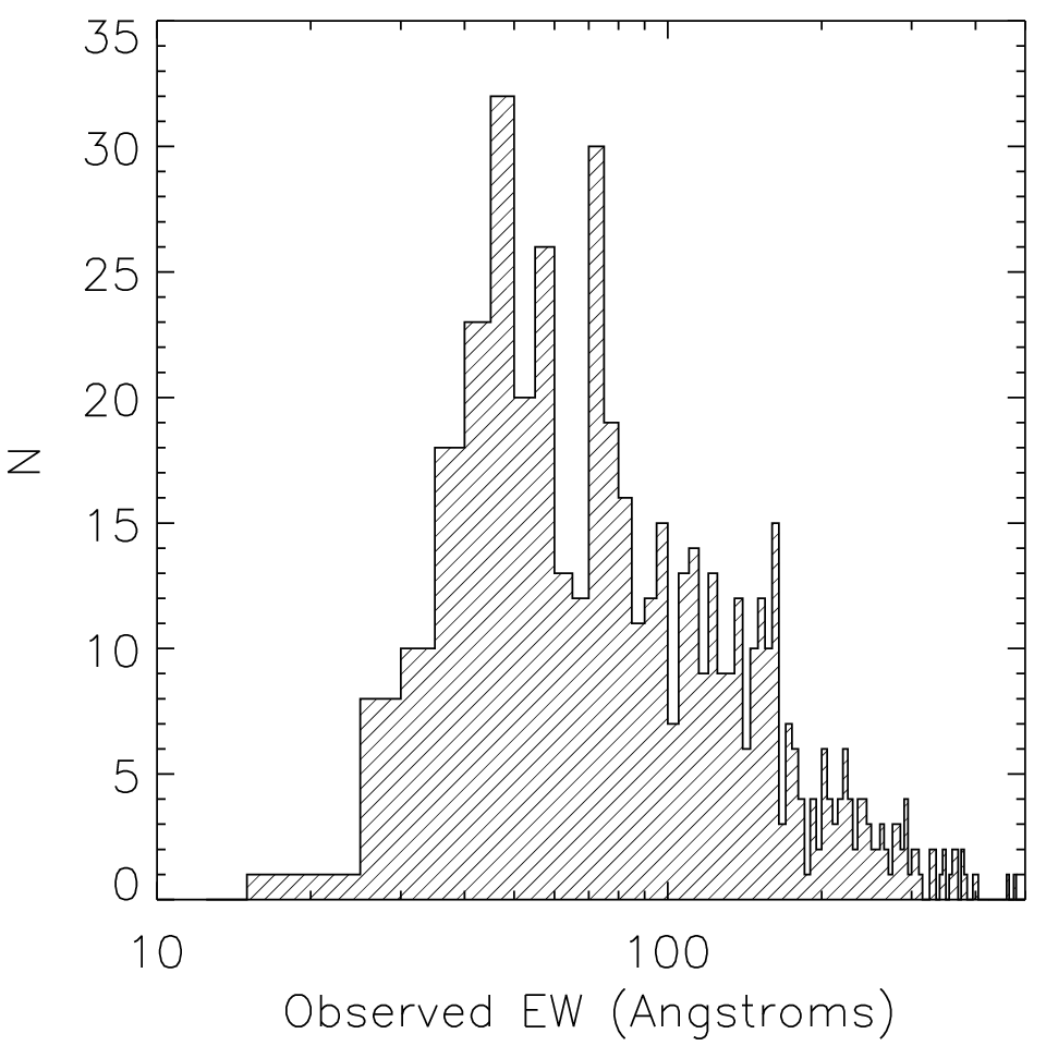
With this equation, the minimum mag excess corresponds to an observed EW of 40 Å. To compute luminosities, we adopt a distance of 5041 Mpc, which corresponds to , the median redshift of our spectroscopically confirmed H emitters. Distributions of the observed emission-line fluxes and EWs for our sample of H emitters are shown in Figure 5.

IV.2. Derived H Luminosities
To determine the intrinsic H luminosity from the observed line luminosity, corrections must be applied for contamination of the flux by the adjacent [N II] lines, and for attenuation by dust internal to the galaxy. The corrections that we adopt are based on standard, empirically calibrated relationships, which describe average corrections for ensemble populations. They should yield luminosities appropriate for computing averaged/integrated quantities such as the SFR volume density. However, it should be noted that the corrections will not be accurate for individual galaxies, since the scatter in the relationships is large, as described below.
[N II] contamination. The NB118 bandpass is wide enough to include flux from the [N II] 6548,658344 4 Hereafter, “[N II]” refers to both nitrogen nebular emission lines. emission lines for narrowband excess selected H emitters.
In the local universe, integrated spectroscopic surveys have found that the H/[N II] flux ratio is 2.3 for typical galaxies [22, 11], and past narrowband surveys have often adopted a fixed correction of 2.3 for all selected H emitters. The flux ratio, however, has been shown to increase with larger emission-line EW [58, see, e.g.,] and with decreasing -band luminosities [25, 30]. Such correlations are likely a consequence of the mass–metallicity relationship [29, 54, e.g.,]. In a recent deep optical narrowband survey with Subaru Suprime-Cam, [33] adopted 4.66 based on optical spectroscopic follow-up of their emitters. The sample of [33] consists of galaxies with fainter luminosities, hence are more metal-poor and would have a higher H/[N II] flux ratio on average.
For this study, we follow 58 and 50 in adopting an EW-dependent H/[N II] flux ratio to facilitate comparisons of results. The EW-dependent correction was constructed from thousands of star-forming galaxies from the Sloan Digital Sky Survey fourth data release with which 58 determined the mean relationship between the rest-frame EW of H + [N II] 6583 and the H/[N II] flux ratio. The correlation exhibits a scatter of 0.2 dex, which implies that estimates of the H/[N II] ratio for individual sources will only be accurate to 50%. Such errors will average out in the calculation of integrated quantities however, and are adequate for our purposes here.
Also, our correction assumes that the H/[N II] relation does not evolve with redshift. This is a valid assumption since the evolution of metallicity between and has been found to be no more than 0.1 dex [see, e.g., 34, and references therein]. Near-infrared multi-object spectroscopy will be needed to examine the H/[N II] ratio for NB selected galaxies on a case-by-case basis. Assuming the 58 [N II] correction, the H/[N II] ratio varies from 1.85 to 10.0 with a median (average) of 2.50 (2.81) for our population of H emitting galaxies.
Dust attenuation. To correct for dust attenuation, we adopt a luminosity-dependent extinction relation following [20]:
| (12) | |||||
[20] showed that attenuations computed from this equation show a 0.2 dex scatter relative to those based on Balmer decrement measurements for individual galaxies. Much like the [N II] correction, these dust extinction corrections are more reliable when considering multiple sources of a given luminosity/SFR. The [20] relation was also adopted in other studies (e.g., Ly et al. 33; 58; Dale et al. 6). For our sample, this correction (A[H]) ranges from 0.66 to 1.87 mag with a median and average of 1.19 and 1.21 mag, respectively.
One piece of evidence that supports the [20] relation is the work of [12], which has looked at the UV, H, and mid-infrared fluxes for a sample of narrow-band selected H emitters to determine dust attenuation. They find a correlation between the observed H luminosity and dust attenuation that is similar to [20]. This multi-wavelength comparison will be conducted for our sample of H emitters. We will also investigate dust attenuation determined from Balmer decrements, which are obtained from the combination of our NB118 measurements and our IMACS follow-up spectroscopy (I. Momcheva et al. 2011, in preparation). Preliminary results do indicate that the attenuations based on Balmer decrements for the NB118-selected H emitters are consistent with the [20] correction.
V. Completeness of the Survey
V.1. Monte Carlo Simulations
Motivation. To account for the detection limits and photometric selection of the NewH survey, we need to estimate the completeness fraction as a function of luminosity, . The greatest uncertainty for such a task is the intrinsic EW distribution, that is, the inherent distribution of the population that we are able to seek. Since the narrowband and broadband imaging sensitivities of the survey are known, the completeness is determined for a source of a given brightness with a excess color (i.e., an EW). However, sources of a given emission-line luminosity can be faint with large EWs or bright with low EWs. Thus, the adopted EW distribution affects the estimated completeness for individual emission-line luminosity bins. For this reason, we conduct Monte Carlo realizations of our data, and follow a “maximum likelihood” approach to determine the completeness of NewH.
Technique/approach. The methodology intends to simultaneously reproduce the shape of the observed55 5 Throughout this section, we use “observed” to denote that the EW distributions are a factor of larger than the rest-frame EW distributions. H+[N II] EW distribution and the observed H LF. We begin with a grid of models that adopt certain EW distributions. With these distributions, we generate artificial emission-line galaxies. We add noise to these galaxies, and use their measured magnitudes and colors to determine if these mock galaxies satisfy the NB118 excess selection. We construct the observed EW distribution and H LF from the sample of mock NB118 excess emitters to compare to the respective distributions from NewH. We determine a best model and define the completeness, , as the ratio of the number of mock NB118 excess emitters to the total number of generated artificial galaxies:
| (13) |
Assumptions. For the prior distributions, we make two assumptions. First, for the H LF, a proper normalization of bright-to-faint sources is necessary, otherwise we will generate relatively too many bright sources, and a decline in the simulated LF will not been seen and cannot be compare to the observed H LF. To constrain the ratio of bright-to-faint sources, we examine the galaxy number counts (N[]) in the NewH fields and find that . This relation implies that the number of galaxies at magnitude is a factor of 2.2 more numerous than those at .
Second, each plausible model assumes a log-normal EW distribution described by a mean and a sigma . We adopt such a distribution, since it is fairly similar to the observed NewH distributions and the distributions seen locally [28]. Our models span –1.55 and –0.40 both in increments of 0.05 dex for a total of 54 EW distributions. Here, is the logarithm of the rest-frame EW, and we later include a factor of 1+ for the “observed” magnitudes, colors, fluxes, and EWs.

Implementation. For each of the 54 models, we generate 40,000 mock galaxies with -band (continuum) magnitudes chosen to follow the above relation between and . We assume that these galaxies are spatially unresolved and follow the FWHM of seeing for each mosaic. For the EWs, we randomly draw from a log-normal distribution given by and . With these two information, we “fill” the color–magnitude diagram ( versus NB118; see Figure 6).
We add observational uncertainties to the and NB118 magnitudes as follows. For each mock galaxy, we have a randomly chosen position in the mosaics, and generate 200 realizations based on the sensitivity at that position. The sensitivity is governed by the exposure maps for both the NB118 and -band mosaics, thus accounting for detector and pixel-to-pixel variations. We compute the NB118 or -band 3 limiting magnitudes, , signal-to-noise ratios, S/N, and 1 uncertainties, , as
| (14) | |||||
| (15) | |||||
| (16) |
where and are the individual detector’s median limiting magnitudes and exposure times (see Table 1), respectively, and is the NB118 or magnitude. For the colors, the errors are added in quadrature: . The magnitudes for the 200 realizations follow a Gaussian distribution with a mean of and 1 of .
We identify mock galaxies that are NB118 excess emitters using the same methods described in Section III.1. For the smaller apertures (2″ or 25), we assume that the flux enclosed is between 81% and 86% of the total flux within the larger apertures (3″ or 4″). We determine these values by considering a Gaussian distribution with a FWHM equal to the seeing size for each NEWFIRM pointing. Note that we adopt limiting magnitudes appropriate for the size of the measurement aperture.
Comparisons with observations. For each model, we construct the observed EW distribution and H LF from the mock NB118 excess emitters. Since we generate many mock galaxies, we normalize each distribution to best match the observed NewH distributions. We illustrate an example of these model–observation comparisons in Figure 7 for the SXDS-W field. We find the best fit by minimizing through a comparison of the mock and the NewH EW distributions and H LFs. We show in Figure 7 that the best-fit model is able to reproduce both the EW distribution and the H LF. We find that observed EW distribution provides a better constraint on the best-fit model (versus the H LF). That is, multiple EW models can sufficiently explain the H LF. We find the model with and best matches the observed distributions.

We calculate the completeness as the ratio of the number of mock galaxies that meets the NB118 excess selection criteria to all mock galaxies () as a function of . We illustrate in Figure 8 how the completeness differs by adopting different values. This comparison shows that we miss bright galaxies with low EWs, which is not surprising given the minimum observed EW of 40 Å. This figure also reveals that the completeness can vary between 60% and 90% for observed fluxes of – erg s-1 cm-2 or roughly 0.1–1 (see Section VI.1), and emphasizes that proper choice in the prior EW distribution is necessary for an accurate determination of the LF. We also show the completeness as a function of H luminosity and observed EW for each of the fields assuming the best-fitting model with and in Figure 9.


Discussion of simplifying assumptions. In the above calculations, we made a couple of simplifications to allow the Monte Carlo simulations to be significantly less computationally intensive. First, we assume that the galaxies are unresolved sources. Second, instead of detecting sources on the images, we estimate the measured magnitudes and fluxes where the photometric uncertainties are based on pixel-to-pixel and detector-dependent sensitivity. Third, it is important to note that our current simulations assume that the EW distribution is the same at all continuum magnitudes. It would be more correct to allow the EW distribution to vary as a function of continuum magnitude, since it has been shown that more luminous star-forming galaxies tend to have lower emission-line EWs than those at lower luminosity [28, e.g.,]. However, this adds another degree of freedom to our models, and significantly increases the computational time required to complete the simulations. Future work will include greater complexity in the modeling of the EW distribution, and will examine the impact of the current assumptions on the resultant completeness corrections. These simplifications allow for a few orders of magnitude faster production of completeness results rather than the approach of adding sources directly to the images, and is able to reproduce the distributions of scatter in Figures 1 and 2 (e.g., see Figure 6).
Prior to these MC simulations (for this discussion, we refer to the above approach as “Method II”), we generated a simulation where artificial extended sources were directly added to the mosaics and detected. In this simulation (referred to as “Method I”), we adopted a log-normal Gaussian EW distribution with and , motivated by the results in [28]. We performed Method I by adding 1000 artificial galaxies to each NEWFIRM mosaic, and compared the number of artificial NB118 excess emitting galaxies to the number detected. We created the galaxies using IRAF/mkobjects with physical parameters similar to those found in local galaxies. The parameters include luminosities, H EWs, semimajor to semiminor axial ratios (between 0.15 and 1.0), and the H disk scale length [4, 3.6 kpc;]. After extracting sources in the same manner described in Section III, we calculated the completeness. We repeated each simulation 30 times using different seed numbers to increase the statistical accuracy of the results ( per NEWFIRM pointing). The similarities in the shape of the completeness curves in Methods I and II suggest that the simplifications we made do not have a significant effect on the estimated completeness. There are certain differences such that the comparison is not completely “apples-to-apples”; however, good agreement suggests that proceeding with Method II is satisfactory. The greatest benefit of this simulation is the determination of a model that best matches two different sets of measurements.
Finally, we assume a power-law distribution for N() to normalize the number of bright and faint sources. Ideally, the distribution should be constructed from galaxies at . An investigation with the COSMOS photo- sample (after the simulation was completed) finds that the faint-end slope of the number counts is approximately 0.25, which is to be compared to the adopted 0.34. Also, an exponential decline exists at bright continuum luminosities. This will impact our completeness estimates for the brightest emitters. Future work will address and examine the impact that these differences have on the completeness reported here.
V.2. Effective Volume
The volume that the survey is capable of probing is determined by the shape and width of the NB filter. The ideal filter will have a perfect top-hat profile, and will survey the same co-moving volume at all emission-line fluxes. However, with real filters a weak emission line can either result from the line falling in the wings of the NB filter profile or from an intrinsically weak line located near the filter center. The net result is that a weak emission line is more likely to be detected near filter center, so a non-square filter reduces the effective volume at the faint end [33].
We can quantify how much the filter profile deviates from being a perfect top-hat by comparing the area underneath the profile with that of a rectangle with width equal to the FWHM, and height equal to the maximum transmission of the actual filter. The area enclosed by the profile is just 9% smaller, so the shape of the bandpass is close to the ideal.
To determine the effective volume as a function of emission-line flux, we calculate the range in wavelengths such that an emission line is considered detectable within the NB filter. This emission line has an intrinsic S/N. We then place it at different wavelengths to determine what the degradation in the S/N will be due to lower throughput. We define an emission line to be undetected below 2.5, and this criterion yields the minimum and maximum NB118 wavelengths (hence redshift) that is observable for a particular S/N. The effective comoving volume per unit steradian would then be
| (17) | |||||
| (18) | |||||
| (19) | |||||
| (20) |
Here, and refer to the minimum and maximum redshifts that the emission line is detectable. Note that these equations assume a flat universe. The maximum surveyed volume ( Mpc3 deg-2 or Å) is observable for and decreases to Mpc3 deg-2 ( Å) at . This is illustrated in Figure 10.

VI. Results
| 2.5 | 3 | ||||||||
|---|---|---|---|---|---|---|---|---|---|
| Raw number densities | |||||||||
| 40.70 | 11 | 0 | 11.173.4 | 0.08 | … | … | … | … | |
| 40.90 | 60 | 8 | 49.346.4 | 0.22 | 20 | 3 | 12.742.8 | 0.22 | |
| 41.10 | 116 | 27 | 83.767.8 | 0.47 | 65 | 19 | 40.365.0 | 0.49 | |
| 41.30 | 102 | 50 | 63.026.2 | 0.72 | 78 | 45 | 45.965.2 | 0.73 | |
| 41.50 | 98 | 74 | 55.395.6 | 0.79 | 96 | 73 | 54.015.5 | 0.79 | |
| 41.70 | 66 | 54 | 36.214.5 | 0.79 | 66 | 54 | 36.214.5 | 0.79 | |
| 41.90 | 34 | 26 | 18.653.2 | 0.81 | 34 | 26 | 18.653.2 | 0.81 | |
| 42.10 | 19 | 18 | 10.422.4 | 0.80 | 19 | 18 | 10.422.4 | 0.80 | |
| 42.30 | 8 | 7 | 4.391.6 | 0.81 | 8 | 7 | 4.391.6 | 0.81 | |
| 42.50 | 8 | 8 | 4.391.6 | 0.86 | 8 | 8 | 4.391.6 | 0.86 | |
| Extinction and completeness-corrected number densities | |||||||||
| 40.90 | 3 | 0 | 59.7934.5 | 0.07 | … | … | … | … | |
| 41.10 | 18 | 1 | 245.4057.8 | 0.14 | 3 | 0 | 43.4825.1 | 0.18 | |
| 41.30 | 55 | 8 | 156.5821.1 | 0.28 | 19 | 4 | 46.4610.7 | 0.26 | |
| 41.50 | 77 | 15 | 108.8212.4 | 0.52 | 43 | 10 | 50.127.6 | 0.53 | |
| 41.70 | 99 | 44 | 93.949.4 | 0.69 | 64 | 37 | 54.586.8 | 0.71 | |
| 41.90 | 89 | 55 | 66.397.0 | 0.78 | 84 | 53 | 61.756.7 | 0.78 | |
| 42.10 | 63 | 48 | 43.665.5 | 0.80 | 63 | 48 | 43.665.5 | 0.80 | |
| 42.30 | 50 | 43 | 34.854.9 | 0.79 | 50 | 43 | 34.854.9 | 0.79 | |
| 42.50 | 29 | 24 | 19.703.7 | 0.81 | 29 | 24 | 19.703.7 | 0.81 | |
| 42.70 | 18 | 14 | 12.322.9 | 0.80 | 18 | 14 | 12.322.9 | 0.80 | |
| 42.90 | 12 | 12 | 8.122.3 | 0.81 | 12 | 12 | 8.122.3 | 0.81 | |
| 43.10 | 5 | 4 | 3.371.5 | 0.81 | 5 | 4 | 3.371.5 | 0.81 | |
| 43.30 | 4 | 4 | 2.461.2 | 0.89 | 4 | 4 | 2.461.2 | 0.89 | |
Note. — is normalized to Mpc-3 dex-1 and luminosities () are given in erg s-1. is the survey completeness fraction defined in Section V.1. Numbers reported in the top half are prior to any completeness corrections while completeness is included for the bottom half. The spectroscopic completeness () as a function of luminosity is shown.
VI.1. Luminosity Function and Star Formation Rate Densities


Figure 11 presents the (observed) H LF for this survey with and without completeness corrections. Applying the necessary completeness corrections and adopting the [20] extinction correction, we have the H LF shown in Figure 12. Both raw, and extinction- and completeness-corrected number densities as a function of luminosity are listed in Table 3. The binned LF can be summed together to obtain a model-free, lower-limit H luminosity density of erg s-1 Mpc-3 [ erg s-1 Mpc-3].
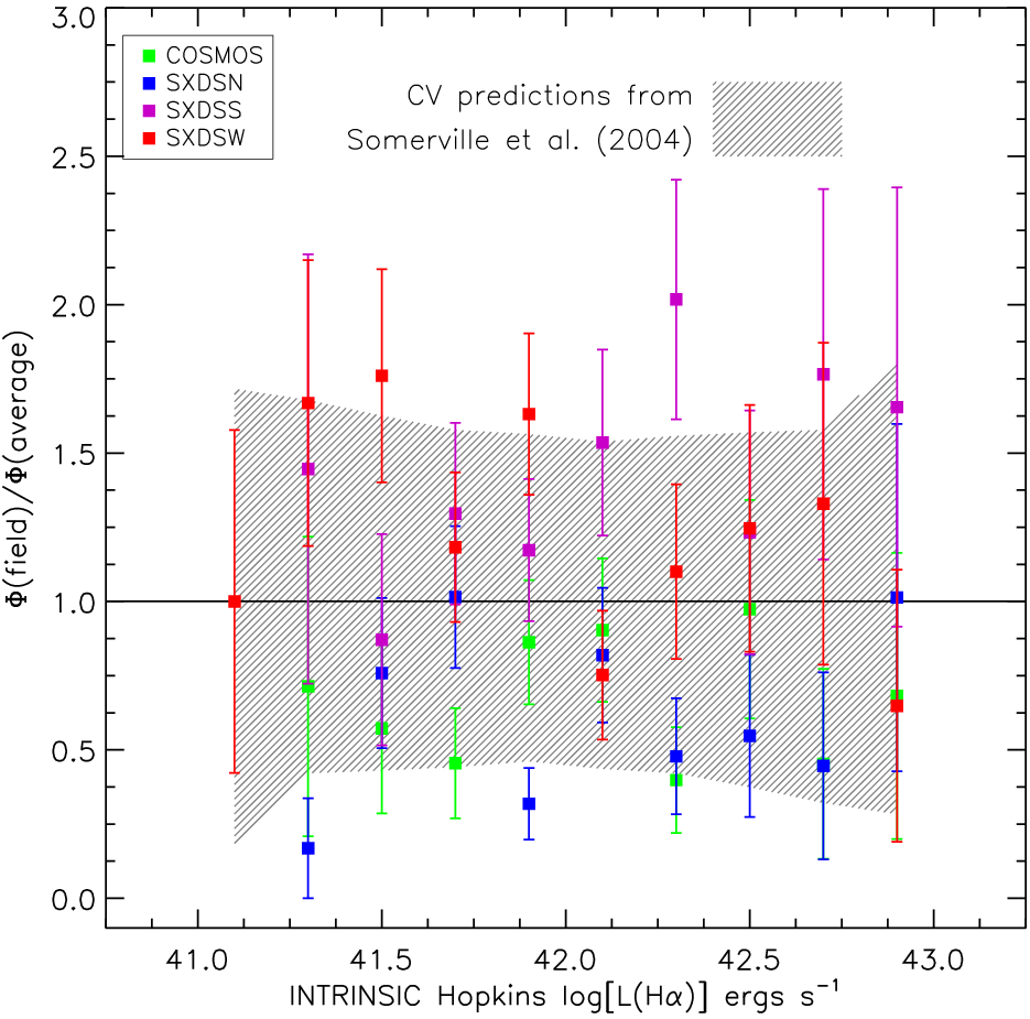
The median variation of the number density relative to the average of all four fields is 50%, and we illustrate in Figure 13 the fluctuation of the four different pointings relative to the average. Using predictions from Somerville et al. [51, hereafter S04], we find that the expected fluctuation per NEWFIRM pointing (shaded region in Figure 13) is consistent with what is observed. The hourglass-like shape of expected amount of field-to-field fluctuations is due to (1) the stronger clustering of luminous galaxies, (2) the decrease of cosmic variance with number density, and (3) the small volume surveyed at low luminosities due to the weakness of emission lines. Thus, the minimum of field-to-field variations is around an extinction-corrected H luminosity of erg s-1.
Note. — and in units of erg s-1 and Mpc-3, respectively. Luminosity () and SFR densities () are provided for and All LFs adopt [20] dust attenuation. Note that 50 incorrectly reported the normalization () for their H LF and was off by a factor of 0.43. D. Sobral provided a new preliminary fit, which adopts the [20] extinction and the proper LF normalization.
It is common to model the H LF by fitting the LF with the [45] function:
| (21) |
This function was derived from the [40] formalism, which describes the halo mass function, and was adapted to explain the distribution of galaxy continuum luminosities. An explanation for why the Schechter function can describe the continuum LF is that a connection exists between the luminosities of galaxies and their stellar masses and/or halo masses. However, such a link may be much weaker with the H luminosity and SFR; thus, one might question whether the Schechter function is a good model for the H LF. For the current analysis we simply assume that the Schechter function can be used to adequately model the distribution of H luminosities and SFR since it appears to provide a good fit to our data. This also facilitates comparisons with previous work. However, this assumption should be explored further when more accurate LFs from future studies show evidence that a Schechter function is not the best model to explain the H LF.
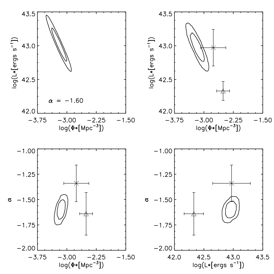
In order to obtain the best-fitting Schechter parameters, a Monte Carlo simulation was performed to consider the full range of scatter in the extinction- and completeness-corrected H LF. We ignored luminosities below our 50% completeness limit ( erg s-1 observed; erg s-1 extinction-corrected). Each datapoint was perturbed randomly times following a Gaussian distribution with in given by Poisson statistics. Each iteration is then fitted to obtain the Schechter parameters. The best-fitting Schechter parameters are then determined from the averages of these fits. The confidence contours for the best fit are shown in Figure 14. A summary of the best fits and the corresponding integrated H luminosity density () and SFR density (see below) is provided in Table 4. We find a relatively steep faint-end slope for the H LF () at , indicating that galaxies below and contribute 61% and 89% to the total H luminosity/SFR density, respectively. Often, past studies have opted to fixed the faint-end slope since they were unable to reliably constrain it. Following this methodology, we also report the results of our fits when is set to 1.6 in Table 4.
The extinction-corrected H luminosity density can be converted into a SFR density by using the recipe given in [23]: SFR(H) = where the SFR is given in yr-1 and the H luminosity is given in erg s-1. This conversion assumes a Salpeter IMF with minimum and maximum masses of 0.1 and 100 and solar metallicity. We determined that the H SFR density is yr-1 Mpc-3 down to , where the second sets of errors account for cosmic variance estimated from 51. Compared to measurements at [10, 39, 3, 37, 16, 33, 59], our H SFR density at is higher by a factor of 3.8 to 16.6 with a median of 8.1.
It is thought that the H luminosity density is dominated by emission from star formation and not active galactic nuclei (AGNs). However, to accurately compute the SFR volume density, we statistically account for the fraction of the H luminosity volume density originating from AGNs. While estimating the AGN fraction is an observational challenge because deep x-ray data and/or spectroscopic information are needed, previous studies have typically found that 10%–15% of galaxies have AGNs. For example, [3] estimate that 11% of the H luminosity density is due to AGNs at . [10] found 15% AGN contamination to the H SFR density at . 58 used X-ray data for a small (50) sample of H emitters at and found 10%3%. 50 looked at the [O III]/H and [O II]/H flux ratios [43], for a subset of 28 H emitters with optical spectroscopy and reported 15%8%. Our preliminary analysis of the rest-frame optical emission-line flux ratios from our IMACS spectroscopy (see Section III.2.1) finds similar results. Based on the [O III]/H and [O II]/H flux ratios, 5 (10) of 141 H emitters are AGNs (LINERs). Thus, we correct the above H SFR density by 11% to account for AGN and LINER contamination. This reduces our total H SFR density to yr-1 Mpc-3.
VII. Comparisons with Other Near-Infrared H Studies
Recently, two other independent groups have performed relatively wide-field near-infrared narrowband imaging on 3–4 m class telescopes to search for high- emission-line galaxies. 58 first surveyed 626 arcmin2 for H emitting galaxies at . They identified 165 galaxies and obtained a extinction-corrected SFR density of 0.17 yr-1 Mpc-3. 50 surveyed a total of 1.3 deg2, identified 743 H emitting galaxies at , and determined a SFR density of 0.1 yr-1 Mpc-3. NewH complements these surveys through a combination of depth and volume surveyed: it covers almost 5 times more area than 58, and while 50 covers about 50% more area, our survey is 0.6 dex deeper. These advantages simultaneously allow us to (1) obtain better constraints on the faint-end slope and “knee” of the LF (we acquired 10% accuracy on the slope and 0.5 dex on ; see above), and to (2) reduce field-to-field fluctuations. The NewH dataset not only enables us to compute a more robust estimate of the LF, it also allows us to better understand the properties of sub- galaxies and their role in the overall star formation history of the universe. Comparisons of the LFs between these three surveys are provided in Figures 11, 12, and 14 and Table 4. We begin by comparing how NB excess emitters are selected and how H emitters are identified, and then discuss the discrepancies between these surveys that are apparent.
Redshift and sensitivity. The 58 and 50 surveys probed volumes at a slightly higher redshift of . Of course, significant evolution between and (corresponding to Myr at Gyr) is not expected. The main consequence of the different surveyed redshift arises from impact of sky background level at the wavelength of redshifted H. NewH targets a cleaner window in the sky spectrum. This partly leads to the factor of two and four times deeper depth in emission-line flux sensitivity compared to 58 and 50.
Selection of excess emitters. All three surveys identify NB excess emitters above significance in the NB color (though we also report results based on a more robust -selected sample). However, there are differences in the minimum NB color criterion and the aperture(s) used. For example, we required at least a (NB118) color of 0.2 mag and used two aperture sizes (2″or 2.5″ and 3 or 4″). 50 used a 3″ diameter selection and required a minimum color of 0.3 mag. 58 indicated that they selected sources in a total of 10 apertures out to 5 times the FWHM with a minimum color of 0.15 mag. We found that the inclusion of larger apertures for NewH only provided 10% more candidates that the smaller aperture failed to catch. Larger apertures would only allow 58 to identify bright and extended galaxies, which are often at lower redshifts.
Identification. In all three surveys, spectroscopic redshift is available for some NB excess emitters to distinguish other emission lines from H. The follow-up spectroscopy that we have classifies 62% [46%] of our 3 [2.5] NB excess emitter candidates. On the other hand, 58 and 50 classified the majority of their NB excess emitters with photometric redshift. These surveys have follow-up spectroscopy for 9% [50, 138/1527;] and 48% [58, 69/165;]. It is difficult to compare directly their spectroscopic completeness against ours since (1) 50 did not report the size of the UDS spectroscopic sample, thus the 9% is a lower limit on their spectroscopic completeness, and (2) 58 only reported spectroscopy for their H emitters rather than the full NB excess emitter sample. For the latter, NewH has 52% spectroscopic completeness of H emitters. Nevertheless, the spectroscopic completeness of NewH is higher than those of 58 and 50.
Similarities in the LF. The observed number density of H emitters is shown in Figure 11 (left panel). It illustrates that all three surveys agree to within 50%, which indicates that the differences in the selection of H emitters and NB excess emitters do not significantly affect the observed number densities of galaxies. The 58 observed LF is generally higher, but it is consistent with our SXDS-S observations, which has a similar area coverage, so cosmic variance is likely the cause (see below for further discussion).
In Figure 12 (right panel) we show the extinction- and completeness-corrected LF for all three H surveys. It is apparent that the bright end of 50’s LF is consistent with NewH’s. This is to be expected since both surveys cover large areas and incompleteness corrections are less of an issue. In addition, 58 is in agreement with NewH below a luminosity of 1042 erg s-1. This is also expected since 58 reaches comparable sensitivity to our survey. However, there are two discrepancies worth addressing.
Differences in the LF. First, the extinction- and completeness-corrected LF of 58 is 0.2–0.3 dex higher at . However, the luminous end of the 58 LF is not well determined since their survey consists of three pointings (two in the Groth strip, one in GOODS-N) totaling less than 0.2 deg2. Thus, the combination of Poisson fluctuations and cosmic variance can explain the higher number density at the bright end.
The second discrepancy is that 50 find a higher number density of faint H emitters, after survey completeness corrections are applied (see Figure 11, right panel). 50 claimed that the completeness correction is a factor of 2–3 at their 2.5 flux limit, while our Monte Carlo simulation indicates that 50% completeness occurs at our flux limit. Furthermore, 50 find that their completeness gradually decline while our Monte Carlo simulation shows that above an observed H emission-line luminosity of erg s-1, the completeness is generally 80% and falls of rapidly with fainter luminosities. How rapidly the completeness declines will affect the shape of the LF, and thus the completeness corrections can alter the determined Schechter parameters. An illustration of this is provided in Figure 14 where the differences in the Schechter parameters for these two studies are shown. Recall that the two LFs prior to any completeness corrections are consistent.
The differences between NewH and 50 at the faint end imply that (1) deeper data must be obtain such that incompleteness determinations are less of an issue or (2) a more standardized rigorous procedure is needed for completeness estimates. For example, a method that considers a maximum likelihood approach that simultaneously produces the observed emission-line EW and LF (such as those performed in Section V.1).
VIII. Discussion

In this section, we compare our H SFR density measurements with those published in the literature for a range of redshifts. We limit the comparison to other H-based measurements to avoid systematic issues with other SFR indicators.
The latest compilation of H measurements was made by [6]. We add our measurements to this compilation and plot them as a function of redshift in Figure 15. All of the measurements plotted are summarized in Table 5. We note that the measurements reported here correct for a few mistakes found in the original papers (see Table 5 footnotes). The dashed line is a fit determined by [6] where the NewH SFR density was not included in the fitting process. It has the form of . Our SFR density measurement with the removal of 11% for AGN contamination is above the [6] fit, but consistent within the uncertainties. This relation indicates that the H SFR density increases by a factor of per unit redshift at .
| References | Areaaafootnotemark: | bbfootnotemark: | ||
|---|---|---|---|---|
| [10] | 0.0220.022 | 471.4 deg2 | 176 | |
| [55] | 0.200.10 | 500 | 138 | |
| [61] | 1.30.5 | 33 | ||
| [52] | 0.150.15 | … | 216 | |
| [56] | 0.730.30 | … | 30 | |
| [8] | 0.2420.009 | 706 | 348 | ccfootnotemark: |
| [18] | 0.2450.007 | 407 | 92 | |
| [39] | 0.0250.025 | … | 79 | |
| [3] | 0.100.01 | SDSS | … | |
| [37] | 0.060.06 | SDSS | 1482 | |
| 0.0790.013 | … | … | ||
| [16] | 0.060.06 | SINGG | 110 | |
| [33] | 0.080.015 | 868 | 318 | ddfootnotemark: |
| 0.240.011 | 868 | 259 | ddfootnotemark: | |
| 0.400.018 | 868 | 391 | ddfootnotemark: | |
| [15] | 2.230.016 | 0.60 deg2 | 55 | eefootnotemark: |
| [36] | 0.2420.009 | 875+SDSS | 575 | |
| [48] | 0.240.009 | 5540 | 980 | |
| 58 | 0.840.009 | 625 | 165 | |
| [60] | 0.240.03 | 1771 | 707 | |
| [47] | 1.10.3 | 35 | ||
| 1.60.3 | 45 | |||
| 50 | 0.840.011 | 1.3 deg2 | 743 | eefootnotemark: |
| [6] | 0.160.02 | 4.19 deg2 | 214 | |
| 0.240.02 | 4.03 deg2 | 424 | ||
| 0.320.02 | 4.13 deg2 | 438 | ||
| 0.400.02 | 1.11 deg2 | 91 | ||
| [17] | 2.190.014 | 56 | 55 | …fffootnotemark: |
| [59] | 0.050.05 | 4 deg2 | 322 | |
| 0.150.05 | 4 deg2 | 1127 | ||
| 0.250.05 | 4 deg2 | 1268 | ||
| 0.340.04 | 4 deg2 | 848 | ||
| NewH (total) | 0.8090.008 | 0.82 deg2 | 522 | ddfootnotemark: |
| NewH ( | 0.8090.008 | 0.82 deg2 | 414 | ddfootnotemark: |
To understand this redshift evolution, we compare in Figure 16 the confidence contours of the Schechter parameters for measurements at , 0.39, and 0.81. The values reported for is based on a combination of data from two complementary surveys: the Subaru Deep Field [SDF; 33, extremely deep for 0.25 deg2] and the Wyoming Survey for H [6, shallower sensitivity by 1.8 dex but covers 1 deg2]. The binned LFs are combined together and fit with a Schechter function. Likewise, measurements from the SDF are combined with [10]. We find that the characteristic luminosity systematically increases by 0.95 dex (0.7 dex) from () to , while the normalization is similar at all three redshifts. This indicates that the increase in the SFR density is a result of galaxies producing stars at a rate that is 10 times that of local ( erg s-1) galaxies.
Infrared surveys have provided complementary constraints on the evolution of the LF and SFR densities. These measurements are sensitive to UV radiation of massive stars that are absorbed by dust and re-radiated at rest wavelengths of 10–100 m. [31] examined the infrared luminosity of 24m-selected galaxies and found that for , the LF evolves as and . These results of significant evolution and weak evolution are consistent with those of NewH, granted this can be for a different population of galaxies.
In addition, we find that our H SFR density measurement at is consistent with UV and [O II] SFR density measurements [19, and references therein], though the scatter among the measurements spans a factor of . The causes for the large scatter include (1) cosmic variance, (2) systematic issues involving the SFR indicators, and (3) the different selection biases that affect each of the surveys. These issues also affect the LF and SFR density derived from infrared surveys. All of these issues will be addressed over the next few years to improve the accuracy that the cosmic star formation history can be determined. In general, cosmic variance will gradually become less of an issue with surveys covering at least several deg2. In future work, data from the NewH survey, in combination with UV data from GALEX, mid-infrared fluxes from Spitzer, and [O II] fluxes from follow-up spectroscopy (see Section III.2.1), will directly enable us to compare the SFRs based on these indicators in hundreds of individual galaxies to address point (2).
And finally, upcoming studies, including ones based upon the NewH Survey, will investigate the differences in galaxy samples that result from the use of different selection techniques. For example, infrared surveys primarily probe the dustiest galaxies, while UV surveys preferentially select the bluest galaxies, and emission-line selected surveys are biased against low-EW galaxies. Direct comparisons of samples selected with different techniques in the same volumes will allow us to account for variations in the SFR volume density, which are due to such selection biases. As mentioned in the Introduction, ultimately it will also be possible to trace large fractions of the cosmic star formation history with a single indicator, and then compare the consistently measured histories from multiple indicators.

IX. Conclusions
We have presented new measurements of the H LF and SFR volume density for galaxies at , based on 1.18m narrowband imaging from the NewH Survey. With a H emission-line flux depth of erg s-1 cm-2 (a luminosity of erg s-1) and an area coverage of 0.82 deg2, the NewH survey allows for a reduction of field-to-field fluctuations to 10%, and for robust estimates of the faint-end slope (10% accuracy) and the location of the “knee” (0.5 dex accuracy) of the LF. We have identified 818 NB excess emitters above 3, and 394 are classified as H emission-line galaxies at . The classification utilized a large spectroscopic sample providing unambiguous determination of redshifts for 62% of the sample. These spectra were also used to calibrate the multi-color selection of the remaining H emitters without spectroscopic follow-up.
We constructed the extinction- and completeness-corrected H LF. Corrections for [N II] flux contamination and the effective surveyed volume, as a function of line flux, were applied. The LF is well described by a Schechter function with erg s-1, Mpc-3, and . When the LF is integrated to , we determine a SFR density of yr-1 Mpc-3. This SFR density is (on average) 8.1 times higher than measurements. We determined that the characteristic H luminosity is systematically higher at by 0.70 and 0.95 dex compared to and estimates, respectively. The normalization of the LF at is similar to what is seen for . This may imply that the cause of the redshift evolution in the H SFR density is a result of galaxies producing stars at a rate that is 10 times that of typical galaxies seen locally.
The depth and completeness of current high- H surveys significantly limit the accuracy to which the (1) H SFR density, (2) the shape of the LF, and (3) its evolution can be measured. This is underscored by the fact that three independent H surveys (including NewH) show excellent agreement in the observed number densities, but exhibit discrepancies at the factor of two level after completeness corrections are applied. These discrepancies lead to different conclusions on the evolution of star-forming galaxies: while NewH shows redshift evolution in , 58 report evolution in both and , and 50 find evolution in . The differences between the results presented here and that of 58 can be attributed to cosmic variance and small number statistics at the luminous end. Fully understanding the differences between our results and that of 50 require a more in-depth comparison of the completeness corrections for both studies. Future surveys probing fainter luminosities, which will circumvent uncertain completeness corrections above emission-line fluxes of erg s-1 cm-2, in combination with rigorous simulations for incompleteness that are consistently applied across studies, will allow for convergence on the true cosmic SFR volume density, and better understand the factors that drive the evolution.
The OH background is the primary limitation for ground-based near-infrared surveys, which explains the historical dearth of H measurements at –0.8 and in the -band window (). These epochs will be studied with the new Hubble/WFC3 infrared grism. For example, [1] has begun a survey, that will yield H SFRs at –1.6 as well as other emission lines (e.g., [O II] and [O III]) out to to probe a significant fraction of the early universe. Both the NB and grism surveys complement one another through a combination of surveyed area, depth, and redshift.
This study illustrates that H can be extended to high redshift, and with more sensitive detectors and wide field coverage in the near future, H measurements for thousands of galaxies at –3 will be possible to trace cosmic star formation history with a consistent SFR indicator over the past 11 billion years.
References
- [1] Atek, H., et al. 2010, ApJ, 723, 104
- [2] Bertin, E., & Arnouts, S. 1996, A&AS, 117, 393
- [3] Brinchmann, J., Charlot, S., White, S. D. M., Tremonti, C., Kauffmann, G., Heckman, T., & Brinkmann, J. 2004, MNRAS, 351, 1151
- [4] Dale, D. A., Giovanelli, R., Haynes, M. P., Hardy, E., & Campusano, L. E. 1999, AJ, 118, 1468
- [5] Dale, D. A., et al. 2008, AJ, 135, 1412
- [6] Dale, D. A., et al. 2010, ApJ, 712, L189
- [7] Dressler, A., Hare, T., Bigelow, B. C., & Osip, D. J. 2006, Proc. SPIE, 6269, 13
- [8] Fujita, S. S., et al. 2003, ApJ, 586, L115
- [9] Furusawa, H., et al. 2008, ApJS, 176, 1
- [10] Gallego, J., Zamorano, J., Aragon-Salamanca, A., & Rego, M. 1995, ApJ, 455, L1
- [11] Gallego, J., Zamorano, J., Rego, M., & Vitores, A. G. 1997, ApJ, 475, 502
- [12] Garn, T., et al. 2010, MNRAS, 402, 2017
- [13] Gavazzi, G., Boselli, A., Pedotti, P., Gallazzi, A., & Carrasco, L. 2002, A&A, 396, 449
- [14] Gawiser, E., et al. 2006, ApJS, 162, 1
- [15] Geach, J. E., Smail, I., Best, P. N., Kurk, J., Casali, M., Ivison, R. J., & Coppin, K. 2008, MNRAS, 388, 1473
- [16] Hanish, D. J., et al. 2006, ApJ, 649, 150
- [17] Hayes, M., Schaerer, D., & stlin, G. 2010, A&A, 509, L5
- [18] Hippelein, H., et al. 2003, A&A, 402, 65
- [19] Hopkins, A. M. 2004, ApJ, 615, 209
- [20] Hopkins, A. M., Connolly, A. J., Haarsma, D. B., & Cram, L. E. 2001, AJ, 122, 288
- [21] Hopkins, A. M., Connolly, A. J., & Szalay, A. S. 2000, AJ, 120, 2843
- [22] Kennicutt, R. C. 1992, ApJ, 388, 310
- [23] Kennicutt, R. C. 1998, ARA&A, 36, 189
- [24] Kennicutt, R. C., Jr., & Kent, S. M. 1983, AJ, 88, 1094
- [25] Kennicutt, R. C., Jr., Lee, J. C., Funes, S. J., José G., Sakai, S., & Akiyama, S. 2008, ApJS, 178, 247
- [26] Kennicutt, R. C., et al. 2009, ApJ, 703, 1672
- [27] Kurucz, R. L. 1979, ApJS, 40, 1
- [28] Lee, J. C., Kennicutt, R. C., Funes, S. J., José G., Sakai, S., & Akiyama, S. 2007, ApJ, 671, L113
- [29] Lee, J. C., Salzer, J. J., & Melbourne, J. 2004, ApJ, 616, 752
- [30] Lee, J. C., et al. 2009, ApJ, 706, 599
- [31] Le Floc’h, E., et al. 2005, ApJ, 632, 169
- [32] Lilly, S. J., et al. 2007, ApJS, 172, 70
- [33] Ly, C., et al. 2007, ApJ, 657, 738
- [34] Mannucci, F., et al. 2009, MNRAS, 398, 1915
- [35] Meurer, G. R., et al. 2006, ApJS, 165, 307
- [36] Morioka, T., Nakajima, A., Taniguchi, Y., Shioya, Y., Murayama, T., & Sasaki, S. S. 2008, PASJ, 60, 1219
- [37] Nakamura, O., Fukugita, M., Brinkmann, J., & Schneider, D. P. 2004, AJ, 127, 2511
- [38] Oke, J. B. 1974, ApJS, 27, 21
- [39] Pérez-González, P. G., Zamorano, J., Gallego, J., Aragón-Salamanca, A., & Gil de Paz, A. 2003, ApJ, 591, 827
- [40] Press, W. H., & Schechter, P. 1974, ApJ, 187, 425
- [41] Probst, R. G., George, J. R., Daly, P. N., Don, K., & Ellis, M. 2008, Proc. SPIE, 7014, 70142S
- [42] Probst, R. G., et al. 2004, Proc. SPIE, 5492, 1716
- [43] Rola, C. S., Terlevich, E., & Terlevich, R. J. 1997, MNRAS, 289, 419
- [44] Salzer, J. J., et al. 2001, AJ, 121, 66
- [45] Schechter, P. 1976, ApJ, 203, 297
- [46] Scoville, N., et al. 2007, ApJS, 172, 1
- [47] Shim, H., Colbert, J., Teplitz, H., Henry, A., Malkan, M., McCarthy, P., & Yan, L. 2009, ApJ, 696, 785
- [48] Shioya, Y., et al. 2008, ApJS, 175, 128
- [49] Skrutskie, M. F., et al. 2006, AJ, 131, 1163
- [50] Sobral, D., et al. 2009, MNRAS, 398, 75 [50]
- [51] Somerville, R. S., Lee, K., Ferguson, H. C., Gardner, J. P., Moustakas, L. A., & Giavalisco, M. 2004, ApJ, 600, L171 [51]
- [52] Sullivan, M., Treyer, M. A., Ellis, R. S., Bridges, T. J., Milliard, B., & Donas, J. 2000, MNRAS, 312, 442
- [53] Taniguchi, Y., et al. 2007, ApJS, 172, 9
- [54] Tremonti, C. A., et al. 2004, ApJ, 613, 898
- [55] Tresse, L., & Maddox, S. J. 1998, ApJ, 495, 691
- [56] Tresse, L., Maddox, S. J., Le Fèvre, O., & Cuby, J.-G. 2002, MNRAS, 337, 369
- [57] van Dokkum, P. G., et al. 2009, PASP, 121, 2
- [58] Villar, V., Gallego, J., Pérez-González, P. G., Pascual, S., Noeske, K., Koo, D. C., Barro, G., & Zamorano, J. 2008, ApJ, 677, 169 [58]
- [59] Westra, E., Geller, M. J., Kurtz, M. J., Fabricant, D. G., & Dell’Antonio, I. 2010, ApJ, 708, 534
- [60] Westra, E., & Jones, D. H. 2008, MNRAS, 383, 339
- [61] Yan, L., McCarthy, P. J., Freudling, W., Teplitz, H. I., Malumuth, E. M., Weymann, R. J., & Malkan, M. A. 1999, ApJ, 519, L47