Next-to-leading order QCD predictions for $A^{0}\gamma$ associated production at the CERN Large Hadron Collider

Liang Dai Affiliation: Department of Physics and State Key Laboratory of Nuclear Physics and Technology, Peking University, Beijing 100871, China Ding Yu Shao Affiliation: Department of Physics and State Key Laboratory of Nuclear Physics and Technology, Peking University, Beijing 100871, China Chong Sheng Li Email: csli@pku.edu.cn Affiliation: Department of Physics and State Key Laboratory of Nuclear Physics and Technology, Peking University, Beijing 100871, China Affiliation: Center for High Energy Physics, Peking University, Beijing 100871, China Jun Gao Affiliation: Department of Physics and State Key Laboratory of Nuclear Physics and Technology, Peking University, Beijing 100871, China Hao Zhang Affiliation: Department of Physics and State Key Laboratory of Nuclear Physics and Technology, Peking University, Beijing 100871, China

August 24, 2026

Abstract

We calculate the complete next-to-leading-order (NLO) QCD corrections (including SUSY QCD corrections) to the inclusive total cross sections of the associated production processes $pp\rightarrow A^{0}\gamma+X$ in the minimal supersymmetric standard model (MSSM) at the CERN Large Hadron Collider (LHC). Our results show that the enhancement of the total cross sections from the NLO QCD corrections can reach $25\%\sim 15\%$ for $200$ GeV $<m_{A}<500$ GeV and $\tan\beta=50$ . The scale dependence of the total cross section is improved by the NLO corrections in general. We also show the Monte Carlo simulation results for the $\tau^{+}\tau^{-}+\gamma$ signature including the complete NLO QCD effects, and find an observable signature above the standard model (SM) background for a normal luminosity of $100$ fb^-1 at the LHC.

pacs

12.38.Bx, 12.60.Jv, 14.80.Da

I INTRODUCTION

Electroweak symmetry breaking (EWSB) plays a key role in the current research of elementary particles. However, the experimental effort to validate the Higgs mechanism on the CERN Large Hadron Collider (LHC) with a center of mass energy $\sqrt{s}=14$ TeV and a luminosity of $100$ fb^-1 per year [1], is a great challenge. In the standard model (SM) of particle physics, there is only one Higgs particle, which is expected to be lurking somewhere close to the experimental lower bound of $114.4$ GeV set by LEP2 [2]. In the minimal supersymmetric standard model (MSSM), two complex Higgs doublets are introduced to eliminate gauge anomaly [3], resulting in two CP-even ( $h^{0},H^{0}$ ) and one CP-odd ( $A^{0}$ ) neutral Higgs bosons, as well as a pair of charged Higgs bosons. The Higgs sector of the MSSM, at leading order, is characterized by two parameters: one is $m_{A}$ the mass of the pseudo-scalar Higgs boson, and the other $\tan\beta$ the ratio of up- and down-Higgs doublet vacuum expectation value (VEV). Particularly, current experiments hint a scenario with large $\tan\beta\gtrsim 45$ and thus large couplings between the pseudo-scalar Higgs and down-type quarks [4].

At the LHC neutral Higgs bosons are mainly produced via gluon-gluon fusion channel $gg\rightarrow\phi$ [5, 6, 7, 8, 9, 10, 11, 12, 13, 14]. The weak boson fusion channel $qq\rightarrow qqV^{*}V^{*}\rightarrow qqh^{0}/qqH^{0}$ [15, 16, 17] as well as the associated production channel with weak bosons [18, 19, 20] also have significant contributions. Other production channels also have been studied, such as Higgs boson pair production [21, 22, 23, 24] and associated production with top quark pair [25, 26, 27, 28]. Nevertheless, the identification of the Higgs signature is difficult due to large QCD backgrounds against various Higgs particle decay modes. Recently, the Higgs boson and photon associated production channel has aroused interest [29]. For neutral Higgs boson and photon associated production, the otherwise dominating gluon fusion channel is forbidden via C-parity conservation, so quark-antiquark annihilation becomes dominant. In the case of CP-odd Higgs $A^{0}$ produced with a photon in a large $\tan\beta$ MSSM scenario, bottom quark annihilation $b\bar{b}\rightarrow A^{0}\gamma$ is of particular importance due to the large Yukawa coupling enhanced by the large $\tan\beta$ . That compensates for the relatively small parton density of the bottom quark and the suppression from the QED vertex. Besides, associated production arising from weak boson fusion has also been studied in Ref. [30].

Since the bottom quark initial state contribution to $A^{0}\gamma$ associated production is sensitive to the bottom quark Yukawa coupling, the measurement of this channel at the LHC can give detailed information of the Higgs coupling to the bottom quark. To provide a precise prediction of this associated production channel, we calculate the NLO QCD corrections to the total cross section and the kinematic distributions. In addition to effects from virtual or real gluons, loop effects from massive supersymmetry particles (the SUSY QCD effects), such as the sbottoms and the gluino, are also considered. Dimensional regularization scheme (DREG) (with naive $\gamma_{5}$ [31]) is adopted to regularize both ultraviolet (UV) and infrared (IR) divergences, which is equivalent to conventional supersymmetry-preserving dimensional reduction scheme (DRED) at the NLO level [32, 33]. For simplicity, we neglect the bottom quark mass except for in the Yukawa coupling. According to the simplified Aivazis-Collins-Olness-Tung scheme [34, 35, 36], such approximation is justified if the bottom quark appears as an initial parton.

The paper is organized as follows. In Sec. II, brief results for leading-order (LO) calculations are presented. In Sec. III, we present detailed calculations of NLO QCD corrections. In Sec. IV, we discuss a Monte Carlo simulation of the Higgs signature from the decay mode $A^{0}\rightarrow\tau^{+}\tau^{-}$ . In Sec. V, we provide numerical results for the total cross section and the differential cross sections with varying model parameters. Monte Carlo simulation results are also shown there.

II LEADING-ORDER CROSS SECTION FOR NEUTRAL HIGGS AND PHOTON ASSOCIATED PRODUCTION

The LO cross section for $pp\rightarrow\gamma A^{0}$ in the MSSM has been studied in Ref. [29]. At tree level the only partonic subprocess is $b(p_{1})\bar{b}(p_{2})\rightarrow\gamma(p_{3})A^{0}(p_{4})$ , and the corresponding two Feynman diagrams are shown in Fig. 1. The gluon-gluon fusion channel $gg\rightarrow\gamma A^{0}$ is forbidden by C-parity conservation [37, 38, 39]. In the tree level result we keep a finite bottom quark mass denoted as $m_{b}$ . The cross section can be written as

d\hat{\sigma}^{LO}=\frac{1}{2\Phi}dPS^{(2)}\overline{|\mathcal{M}^{B}|^{2}},

(1)

where $dPS^{(2)}$ is the 2-body final-state phase space and $1/2\Phi$ is the flux factor. The explicit expression for the differential cross section after averaging over spins and colors can be written as

\frac{d\hat{\sigma}}{d\hat{t}}=\frac{\alpha_{em}Q_{b}^{2}\lambda_{\phi}^{2}}{4N_{c}(1-4r_{b})}\Big\{\frac{F_{1}^{\phi}(\hat{s})}{(\hat{t}-m_{b}^{2})(\hat{u}-m_{b}^{2})}+F_{2}^{\phi}(\hat{s})\Big[\frac{1}{(\hat{t}-m_{b}^{2})^{2}}+\frac{1}{(\hat{u}-m_{b}^{2})^{2}}\Big]\Big\},

(2)

with

F_{1}^{\phi}(\hat{s})=(1-r_{\phi})^{2}+2r_{\phi}(1-2r_{b}),\qquad F_{2}^{\phi}(\hat{s})=-2r_{b}r_{\phi},

(3)

where $Q_{b}=-1/3$ is the electric charge quantum number of the bottom quark, $N_{c}$ the number of quark color, $r_{b}=m_{b}^{2}/\hat{s},$ $r_{\phi}=m_{A}^{2}/\hat{s}$ , and $\lambda_{\phi}=-i\frac{m_{b}}{v}\tan\beta$ is the Yukawa coupling in MSSM which is proportional to the bottom quark mass. Here $v=2m_{W}/g$ is the SM Higgs field VEV. In addition, the Mandelstam variables for $2\rightarrow 2$ scattering process are introduced

\hat{s}=(p_{1}+p_{2})^{2},\qquad\hat{t}=(p_{1}-p_{3})^{2},\qquad\hat{u}=(p_{1}-p_{4})^{2}.

(4)

The hadronic cross section for $pp\rightarrow\gamma A^{0}$ at the LO is obtained straightforwardly by convoluting the parton level cross section with the parton distribution function (PDF),

\sigma^{B}=\int dx_{1}dx_{2}\big[G_{b/p}(x_{1},\mu_{F})G_{\bar{b}/p}(x_{2},\mu_{F})+(x_{1}\leftrightarrow x_{2})\big]\hat{\sigma}^{B},

(5)

where $\mu_{F}$ is the factorization scale.

Refer to caption — Figure 1: Tree level Feynman diagrams for $b\bar{b}\rightarrow\gamma A^{0}$

III NLO QCD calculations

The NLO QCD correction to $\gamma A^{0}$ associated production consists of two parts. The virtual corrections account for virtual gluons as well as virtual supersymmetric particles such as the gluino $\tilde{g}$ and the sbottoms $\tilde{b}_{1,2}$ in the loop diagrams. The real corrections result from the radiation of a real gluon or a massless bottom (anti-)quark. For the NLO calculations we follow the convention to work in $D=4-2\epsilon$ dimensions and adopt the dimensional regularization approach (DREG) to regulate both the ultroviolet (UV) and the infrared (IR) divergences. As a good approximation, we take the bottom (anti-)quark mass to be zero except for in the Yukawa coupling.

III.1 Virtual corrections

The one-loop virtual corrections involve both the SM QCD contribution (8 diagrams as shown in Fig.2) and the SUSY QCD contribution (another 8 diagrams as shown in Fig.3). Either part is UV divergent. For the gluon loops we adopt $\overline{MS}$ renormalization scheme to absorb those infinities, while for the SUSY particle loops we use the on-shell renormalization scheme instead.

The virtual correction is given by interfering the one-loop amplitude with the Born amplitude

d\hat{\sigma}^{V}=\frac{1}{2\hat{s}}dPS^{(2)}2Re(\overline{\mathcal{M}^{V}\cdot\mathcal{M}^{B}}),

(6)

where $dPS^{(2)}$ is the 2-body final-state phase space and the flux factor is reduced to $1/2\hat{s}$ for massless (anti-)quark. In order to absorb all UV divergences, we introduce the renormalized bottom quark wavefunction for both the left-handed and the right-handed components $\psi_{bL,R}$ and the renormalized mass $m_{b}$ , which are related to the bare mass $m_{b0}$ and the bare wavefunction $\psi_{b0}$ by

	$\displaystyle m_{b0}$	$\displaystyle=m_{b}+\delta m_{b},$
	$\displaystyle\psi_{b0}$	$\displaystyle=(1+\delta Z_{bL})^{1/2}\psi_{bL}+(1+\delta Z_{bR})^{1/2}\psi_{bR},$		(7)

with $\psi_{bL,R}=(1\mp\gamma_{5})\psi_{b}/2$ . By calculating the self-energy diagrams of the bottom quark propagator (shown in Fig.4), we obtain explicit expressions for the counter-terms which are in accordance with the results in Ref. [40, 41],

$\displaystyle\Big(\frac{\delta m_{b}}{m_{b}}\Big)_{SM}$	$\displaystyle=-\frac{\alpha_{s}}{4\pi}C_{F}C(\epsilon)\frac{3}{\epsilon_{UV}},$
$\displaystyle(\delta Z_{bL})_{SM}$	$\displaystyle=(\delta Z_{bR})_{SM}=\frac{\alpha_{s}}{4\pi}C_{F}C(\epsilon)\Big\{-\frac{3}{\epsilon_{UV}}+\frac{3}{\epsilon_{IR}}\Big\},$
$\displaystyle\Big(\frac{\delta m_{b}}{m_{b}}\Big)_{SUSY}$	$\displaystyle=-\frac{\alpha_{s}}{4\pi}C_{F}\underset{i=1,2}{\sum}\big\{B_{1}(0,m_{\tilde{g}}^{2},m_{\tilde{b}_{i}}^{2})-\frac{m_{\tilde{g}}}{m_{b}}\sin 2\theta_{\tilde{b}}(-1)^{i}B_{0}(0,m_{\tilde{g}}^{2},m_{\tilde{b}_{i}}^{2})\big\},$	(8)
$\displaystyle(\delta Z_{bL})_{SUSY}$	$\displaystyle=\frac{\alpha_{s}}{2\pi}C_{F}\underset{i=1,2}{\sum}(R_{i1}^{\tilde{b}})^{2}B_{1}(0,m_{\tilde{g}}^{2},m_{\tilde{b}_{i}}^{2}),$
$\displaystyle(\delta Z_{bR})_{SUSY}$	$\displaystyle=\frac{\alpha_{s}}{2\pi}C_{F}\underset{i=1,2}{\sum}(R_{i2}^{\tilde{b}})^{2}B_{1}(0,m_{\tilde{g}}^{2},m_{\tilde{b}_{i}}^{2}),$

where $C_{F}=4/3$ , $C(\epsilon)=\frac{\Gamma(1-\epsilon)}{\Gamma(1-2\epsilon)}(\frac{4\pi\mu_{R}^{2}}{\hat{s}})^{\epsilon}$ and $B_{0,1}$ are the two-point integrals [42] , as listed explicitly below

	$\displaystyle B_{0}(0,m_{1}^{2},m_{2}^{2})$	$\displaystyle=C(\epsilon)\Big\{\frac{1}{\epsilon_{UV}}-\frac{m_{1}^{2}\ln\frac{m_{1}^{2}}{\hat{s}}-m_{2}^{2}\ln\frac{m_{2}^{2}}{\hat{s}}}{m_{1}^{2}-m_{2}^{2}}+1\Big\},$
	$\displaystyle B_{1}(0,m_{1}^{2},m_{2}^{2})$	$\displaystyle=C(\epsilon)\Big\{-\frac{1}{2\epsilon_{UV}}+\frac{2m_{1}^{4}\ln\frac{m_{1}^{2}}{\hat{s}}-3m_{1}^{4}+4m_{1}^{2}m_{2}^{2}-m_{2}^{4}+2m_{2}^{2}(m_{2}^{2}-2m_{1}^{2})\ln\frac{m_{2}^{2}}{\hat{s}}}{4(m_{1}^{2}-m_{2}^{2})^{2}}\Big\},$		(9)

where $m_{\tilde{b}_{1,2}}$ are the sbottom masses, $m_{\tilde{g}}$ is the gluino mass, and $R^{\tilde{b}}$ is a $2\times 2$ rotation matrix which transforms the gauge eigenstates into the mass eigenstates,

\left(\begin{array}[]{c}\tilde{b}_{1}\\ \tilde{b}_{2}\end{array}\right)=R^{\tilde{b}}\left(\begin{array}[]{c}\tilde{b}_{L}\\ \tilde{b}_{R}\end{array}\right),\qquad R^{\tilde{b}}=\left(\begin{array}[]{cc}\cos\theta_{\tilde{b}}&\sin\theta_{\tilde{b}}\\ -\sin\theta_{\tilde{b}}&\cos\theta_{\tilde{b}}\end{array}\right),

(10)

with $0\leq\theta_{\tilde{b}}\leq\pi$ by convention. Furthermore, the sbottom mass eigenvalues are solved by diagonalizing $M_{\tilde{b}}^{2}$ ,

\left(\begin{array}[]{cc}m_{\tilde{b}_{1}}^{2}&0\\ 0&m_{\tilde{b}_{2}}^{2}\end{array}\right)=R^{\tilde{b}}M_{\tilde{b}}^{2}(R^{\tilde{b}})^{\dagger},\qquad M_{\tilde{b}}^{2}=\left(\begin{array}[]{cc}m_{\tilde{b}_{L}}^{2}&a_{b}m_{b}\\ a_{b}m_{b}&m_{\tilde{b}_{R}}^{2}\end{array}\right),

(11)

with

	$\displaystyle m_{\tilde{b}_{L}}^{2}=M_{\tilde{Q}}^{2}+m_{b}^{2}+m_{Z}^{2}\cos 2\beta C_{bL},$
	$\displaystyle m_{\tilde{b}_{R}}^{2}=M_{\tilde{D}}^{2}+m_{b}^{2}-m_{Z}^{2}\cos 2\beta C_{bR},$
	$\displaystyle a_{b}=A_{b}-\mu\tan\beta.$		(12)

Here $C_{bL}=-1/2+\sin^{2}\theta_{W}/3$ , $C_{bR}=\sin^{2}\theta_{W}/3$ , and $M_{\tilde{b}}^{2}$ is the sbottom mass matrix. $M_{\tilde{Q},\tilde{D}}^{2}$ and $A_{b}$ are soft SUSY-breaking parameters, and $\mu$ is the Higgsino mass parameter. Since the Yukawa coupling is proportional to the bottom quark mass, the renormalized vertex is obtained by expressing the bare mass $m_{b0}$ in terms of the renormalized mass $m_{b}$ plus a counter term $\delta m_{b}$ ,

-i\frac{m_{b0}}{v}\tan\beta=-i\Big[1+\Big(\frac{\delta m_{b}}{m_{b}}\Big)_{SM}+\Big(\frac{\delta m_{b}}{m_{b}}\Big)_{SUSY}\Big]\frac{m_{b}}{v}\tan\beta.

(13)

All the counter-term diagrams are shown in Fig.5.

With the one-loop counter-terms we write the renormalized virtual amplitude as

\mathcal{M}^{V}=\mathcal{M}_{SM}^{unren}+\mathcal{M}_{SUSY}^{unren}+\mathcal{M}^{con}.

(14)

The details of the calculation include the traditional Passarino-Veltman reduction procedure, in which Feynman amplitudes are reduced to master scalar integrals [43]. Here we list the analytic results for all the divergent scalar integrals (only the real part is kept) involved in the calculation,

$\displaystyle B_{0}(\hat{t},0,0)=$	$\displaystyle C(\epsilon)\Big[\frac{1}{\epsilon_{UV}}+2-\ln\Big(\frac{-\hat{t}}{\hat{s}}\Big)\Big],$
$\displaystyle B_{0}(\hat{u},0,0)=$	$\displaystyle C(\epsilon)\Big[\frac{1}{\epsilon_{UV}}+2-\ln\Big(\frac{-\hat{u}}{\hat{s}}\Big)\Big],$
$\displaystyle B_{0}(m_{A}^{2},0,0)=$	$\displaystyle C(\epsilon)\Big[\frac{1}{\epsilon_{UV}}+2-\ln r_{\phi}\Big],$
$\displaystyle C_{0}(0,0,\hat{t},0,0,0)=$	$\displaystyle C(\epsilon)\Big(\frac{1}{-\hat{t}}\Big)\Big[-\frac{1}{\epsilon_{IR}^{2}}+\frac{\ln(-\hat{t}/\hat{s})}{\epsilon_{IR}}-\frac{1}{2}\ln^{2}\Big(\frac{-\hat{t}}{\hat{s}}\Big)-\frac{\pi^{2}}{6}\Big],$
$\displaystyle C_{0}(0,0,\hat{u},0,0,0)=$	$\displaystyle C(\epsilon)\Big(\frac{1}{-\hat{u}}\Big)\Big[-\frac{1}{\epsilon_{IR}^{2}}+\frac{\ln(-\hat{u}/\hat{s})}{\epsilon_{IR}}-\frac{1}{2}\ln^{2}\Big(\frac{-\hat{u}}{\hat{s}}\Big)-\frac{\pi^{2}}{6}\Big],$
$\displaystyle C_{0}(0,m_{A}^{2},\hat{s},0,0,0)=$	$\displaystyle C(\epsilon)\Big(\frac{1}{1-r_{\phi}}\Big)\Big[\frac{\ln r_{\phi}}{\epsilon_{IR}}-\frac{\ln^{2}r_{\phi}}{2}\Big],$
$\displaystyle C_{0}(0,m_{A}^{2},\hat{t},0,0,0)=$	$\displaystyle C(\epsilon)\Big(\frac{1}{m_{A}^{2}-\hat{t}}\Big)\Big[\frac{1}{\epsilon_{IR}}\ln\Big(\frac{-\hat{t}}{m_{A}^{2}}\Big)-\frac{1}{2}\ln r_{\phi}\ln\Big(\frac{-\hat{t}}{m_{A}^{2}}\Big)$
	$\displaystyle-\frac{1}{2}\ln\Big(\frac{-\hat{t}}{\hat{s}}\big)\ln\Big(\frac{-\hat{t}}{m_{A}^{2}}\Big)-\frac{\pi^{2}}{2}\Big],$
$\displaystyle C_{0}(0,m_{A}^{2},\hat{u},0,0,0)=$	$\displaystyle C(\epsilon)\Big(\frac{1}{m_{A}^{2}-\hat{u}}\Big)\Big[\frac{1}{\epsilon_{IR}}\ln\Big(\frac{-\hat{u}}{m_{A}^{2}}\Big)-\frac{1}{2}\ln r_{\phi}\ln\Big(\frac{-\hat{u}}{m_{A}^{2}}\Big)$	(15)
	$\displaystyle-\frac{1}{2}\ln\Big(\frac{-\hat{u}}{\hat{s}}\big)\ln\Big(\frac{-\hat{u}}{m_{A}^{2}}\Big)-\frac{\pi^{2}}{2}\Big],$
$\displaystyle D_{0}(0,m_{A}^{2},0,0,\hat{t},\hat{s},0,0,0,0)=$	$\displaystyle C(\epsilon)\Big(\frac{1}{-\hat{t}}\Big)\Big[-\frac{2}{\epsilon_{IR}^{2}}+\frac{2}{\epsilon_{IR}}\ln\Big(\frac{-\hat{t}}{m_{A}^{2}}\Big)+\ln r_{\phi}^{2}$
	$\displaystyle+2\Big({\rm{Li}}_{2}\Big(\frac{\hat{s}-m_{A}^{2}}{\hat{s}}\Big)-{\rm{Li}}_{2}\Big(\frac{\hat{s}-m_{A}^{2}}{\hat{t}}\Big)\Big)-\pi^{2}\Big],$
$\displaystyle D_{0}(0,m_{A}^{2},0,0,\hat{u},\hat{s},0,0,0,0)=$	$\displaystyle C(\epsilon)\Big(\frac{1}{-\hat{u}}\Big)\Big[-\frac{2}{\epsilon_{IR}^{2}}+\frac{2}{\epsilon_{IR}}\ln\Big(\frac{-\hat{u}}{m_{A}^{2}}\Big)+\ln r_{\phi}^{2}$
	$\displaystyle+2\Big({\rm{Li}}_{2}\Big(\frac{\hat{s}-m_{A}^{2}}{\hat{s}}\Big)-{\rm{Li}}_{2}\Big(\frac{\hat{s}-m_{A}^{2}}{\hat{u}}\Big)\Big)-\pi^{2}\Big],$

We then find that the renormalized amplitude $\mathcal{M}^{V}$ is UV finite, but still contains IR poles, which is given by

\mathcal{M}^{V}=\frac{\alpha_{s}}{2\pi}C(\epsilon)\Big\{\frac{A_{2}^{V}}{\epsilon_{IR}^{2}}+\frac{A_{1}^{V}}{\epsilon_{IR}}\Big\}\mathcal{M}^{B},

(16)

with

A_{2}^{V}=-C_{F},\qquad A_{1}^{V}=-\frac{3}{2}C_{F},

(17)

which demonstrates that the IR divergent part is factorized and consists of both soft and collinear singularities. The former is canceled when we combine the virtual corrections with the real corrections, while the latter can be canceled by adopting the mass factorization procedure.

III.2 Real gluon emission

The Feynman diagrams for the radiation of a real gluon $b(p_{1})\bar{b}(p_{2})\rightarrow\gamma(p_{3})A^{0}(p_{4})g(p_{5})$ are shown in Fig.6. The partonic cross section can be written as

d\hat{\sigma}^{R}=\frac{1}{2\hat{s}}dPS^{(3)}\overline{|\mathcal{M}^{B}|^{2}},

(18)

The 3-body phase space integration for real gluon emission contains soft and collinear singularities. We adopt the two cutoff phase space slicing method [44] to isolate all the IR singularities, which introduces two small cutoffs $\delta_{s}$ and $\delta_{c}$ to divide the phase space into three parts.

First, the soft cutoff $\delta_{s}$ separates the phase space into the soft region $E_{5}\leq\delta_{s}\sqrt{\hat{s}}/2$ and the hard region otherwise in the partonic center of mass (CM) frame. Thus the partonic cross section can be written as a sum of the contributions from both regions,

\hat{\sigma}^{R}=\hat{\sigma}^{S}+\hat{\sigma}^{H}.

(19)

Furthermore, the hard piece can be divided into two sub-regions by introducing a collinear cutoff $\delta_{c}$ . Within the hard collinear region $(p_{1}+p_{5})^{2}\leq\delta_{c}\hat{s}$ or $(p_{2}+p_{5})^{2}\leq\delta_{c}\hat{s}$ all the collinear divergences are isolated, leaving the hard non-collinear region free of any IR singularities. Similarly we have for the partonic cross section

\hat{\sigma}^{H}=\hat{\sigma}^{HC}+\hat{\sigma}^{\overline{HC}}.

(20)

Below we proceed to discuss the details of calculation in each region of the phase space.

III.2.1 Hard non-collinear region

For the hard non-collinear region where no IR singularity is present, the phase space integration can be calculated numerically. For the 3-body phase space a convenient parameterization with 4 non-trivial parameters is given below,

dPS^{(3)}=\frac{\hat{s}}{32(2\pi)^{4}}dX_{1}dX_{2}d\cos\theta d\varphi.

(21)

Here $-1\leq\cos\theta\leq 1$ and $0\leq\varphi\leq 2\pi$ represent the solid angle in the CM frame into which the final-state photon is scattered. Besides, $X_{1,2}$ are dimensionless variables which determine the final state energy in the partonic CM frame through

E_{3}=\frac{\sqrt{\hat{s}}}{2}(1-X_{2}),\qquad E_{4}=\frac{\sqrt{\hat{s}}}{2}(X_{1}+X_{2}),\qquad E_{5}=\frac{\sqrt{\hat{s}}}{2}(1-X_{1}).

(22)

The integration region for them is inside the unit square in the parameter plane and are subject to kinematic constraints $X_{1}+X_{2}\leq 1+r_{\phi}$ and $X_{1}X_{2}\geq r_{\phi}$ .

III.2.2 Soft region

In the limit of vanishing gluon energy (the eikonal approximation), the squared matrix element for real gluon emission can be factorized into the Born piece multiplied by an eikonal factor $\Phi_{eik}$

\overline{|\mathcal{M}^{R}(b\bar{b}\rightarrow\gamma A^{0}+g)|^{2}}\overset{soft}{\longrightarrow}(4\pi\alpha_{s}\mu_{R}^{2\epsilon})\overline{|\mathcal{M}^{B}|^{2}}\Phi_{eik},

(23)

where the eikonal factor can be written explicitly

\Phi_{eik}=C_{F}\Big\{\frac{-p_{1}^{2}}{(p_{1}\cdot p_{5})^{2}}+\frac{-p_{2}^{2}}{(p_{2}\cdot p_{5})^{2}}+\frac{2(p_{1}\cdot p_{2})}{(p_{1}\cdot p_{5})(p_{2}\cdot p_{5})}\Big\}=C_{F}\frac{\hat{s}}{(p_{1}\cdot p_{5})(p_{2}\cdot p_{5})}.

(24)

Meanwhile the 3-body phase space is factorized into the following form

dPS^{(3)}(b\bar{b}\rightarrow\gamma A^{0}+g)\overset{soft}{\longrightarrow}dPS^{(2)}(b\bar{b}\rightarrow\gamma A^{0})dS,

(25)

with $dS$ the soft gluon phase space to be integrated

dS=\frac{1}{\pi}(\frac{4}{\hat{s}})^{-\epsilon}\int_{0}^{\delta_{s}\sqrt{\hat{s}}/2}dE_{5}E_{5}^{1-2\epsilon}\int_{0}^{\pi}\sin^{1-2\epsilon}\varphi_{1}d\varphi_{1}\int_{0}^{\pi}\sin^{-2\epsilon}\varphi_{2}d\varphi_{2}.

(26)

After performing the integrations we arrive at a form where IR singularities are explicit

d\hat{\sigma}^{S}=d\hat{\sigma}^{B}\frac{\alpha_{s}}{2\pi}C(\epsilon)\Big(\frac{A_{2}^{S}}{\epsilon^{2}}+\frac{A_{1}^{S}}{\epsilon}+A_{0}^{S}\Big),

(27)

with

A_{2}^{S}=2C_{F},\qquad A_{1}^{S}=-4C_{F}\ln\delta_{s},\qquad A_{0}^{S}=4C_{F}\ln^{2}\delta_{s}.

(28)

III.2.3 Hard collinear region

In the hard collinear region, the factorization theorem [45, 46] states that the squared amplitude can be factorized into the squared Born amplitude multiplied by the unregulated Altarelli-Parisi splitting function as long as the matrix element is calculated under the collinear limit of kinematic configuration.

\overline{|\mathcal{M}^{R}(b\bar{b}\rightarrow\gamma A^{0}+g)|^{2}}\overset{coll.}{\longrightarrow}(4\pi\alpha_{s}\mu_{R}^{2\epsilon})\overline{|\mathcal{M}^{B}(b^{\prime}\bar{b}\rightarrow\gamma A^{0};\hat{s}^{\prime}=z\hat{s})|^{2}}\frac{-2P_{b^{\prime}b}(z,\epsilon)}{z(p_{1}-p_{5})^{2}}.

(29)

Moreover, the phase space can also be factorized in the collinear limit,

dPS^{(3)}(b\bar{b}\rightarrow\gamma A^{0}+g)\overset{coll.}{\longrightarrow}dPS^{(2)}(b^{\prime}\bar{b}\rightarrow\gamma A^{0})\frac{(4\pi)^{\epsilon}}{16\pi^{2}\Gamma(1-\epsilon)}dzdt_{15}\big[-(1-z)t_{15}\big]^{-\epsilon},

(30)

with $t_{15}=(p_{1}-p_{5})^{2}$ . After convoluting with the PDFs we obtain an expression for the inclusive cross section where collinear singularities are explicit in terms of $1/\epsilon$ poles [44]

d\sigma^{HC}_{b-{\rm{splitting}}}=d\hat{\sigma}^{B}(b\bar{b}\rightarrow\gamma A^{0})\Big[G_{b/p}\big(\frac{x_{1}}{z}\big)G_{\bar{b}/p}(x_{2})+(x_{1}\leftrightarrow x_{2})\Big]\\ \times\frac{\alpha_{s}}{2\pi}C(\epsilon)\Big(\frac{1}{-\epsilon}\Big)\delta_{c}^{-\epsilon}P_{bb}(z,\epsilon)\frac{dz}{z}\Big(\frac{1-z}{z}\Big)^{-\epsilon}dx_{1}dx_{2}.

(31)

A similar term which gives exactly the same contribution is also present to account for initial-state anti-quark splitting. So the complete collinear piece is

d\sigma^{HC}=\Big[G_{b/p}\big(\frac{x_{1}}{z}\big)G_{\bar{b}/p}(x_{2})+G_{\bar{b}/p}\big(\frac{x_{1}}{z}\big)G_{b/p}(x_{2})+(x_{1}\leftrightarrow x_{2})\Big]d\hat{\sigma}^{B}(b\bar{b}\rightarrow\gamma A^{0})\\ \times\frac{\alpha_{s}}{2\pi}C(\epsilon)\Big(\frac{1}{-\epsilon}\Big)\delta_{c}^{-\epsilon}P_{bb}(z,\epsilon)\frac{dz}{z}\Big(\frac{1-z}{z}\Big)^{-\epsilon}dx_{1}dx_{2},

(32)

where the unregulated Altarelli-Parisi splitting functions are written explicitly as

P_{bb}(z,\epsilon)=P_{\bar{b}\bar{b}}(z,\epsilon)=C_{F}\Big(\frac{1+z^{2}}{1-z}-\epsilon(1-z)\Big).

(33)

where $G_{b(\bar{b})/p}(x)$ is temporarily the bare PDF. Due to the non-soft constraint we have $x_{1}\leq z\leq 1-\delta_{s}$ .

III.3 Massless bottom (anti-)quark emission

At $\mathcal{O}(\alpha_{s})$ of the perturbative expansion $bg$ (or $\bar{b}g$ ) initial subprocesses should be taken into consideration, with the relevant Feynman diagrams shown in Fig.7.

The treatment is much the same as to $b\bar{b}$ annihilation except for some differences. First, the radiation of a massless (anti-)quark contains no soft divergence. Hence there is no need to introduce a soft cutoff, and the 3-body phase space is divided into a collinear region and a non-collinear region, for the latter numerical calculation is straightforward. There is also collinear singularity arising from collinear emission of massless (anti-)quark. The factorization treatment in the previous subsection applies if we introduce the collinear cutoff $\delta_{c}$ to separate the collinear region and isolate the collinear poles. Combining the non-collinear piece and collinear piece we obtain the cross section

d\sigma^{add.}=\underset{\alpha=b,\bar{b}}{\sum}d\hat{\sigma}^{\overline{C}}(g\alpha\rightarrow\gamma A^{0}+\alpha)\big[G_{g/p}(x_{1})G_{\alpha/p}(x_{2})+(x_{1}\leftrightarrow x_{2})\big]dx_{1}dx_{2}\\ +d\hat{\sigma}^{B}(b\bar{b}\rightarrow\gamma A^{0})\frac{\alpha_{s}}{2\pi}C(\epsilon)\Big(-\frac{1}{\epsilon}\Big)\delta_{c}^{-\epsilon}\Big[P_{bg}(z,\epsilon)G_{g/p}\Big(\frac{x_{1}}{z}\Big)G_{\bar{b}/p}(x_{2})+P_{\bar{b}g}(z,\epsilon)G_{g/p}\Big(\frac{x_{1}}{z}\Big)G_{b/p}(x_{2})\\ +(x_{1}\leftrightarrow x_{2})\Big]\times\frac{dz}{z}\Big(\frac{1-z}{z}\Big)^{-\epsilon}dx_{1}dx_{2},

(34)

where the unregulated Altarelli-Parisi splitting functions are written explicitly as

P_{bg}(z,\epsilon)=P_{\bar{b}g}(z,\epsilon)=\frac{3}{8}C_{F}\big(z^{2}+(1-z)^{2}-2z(1-z)\epsilon\big).

(35)

Further collinear singularity can still arise in the configuration in which the photon is emitted in parallel with the additional final-state quark. By comparison, such singularity does not exist for a final-state gluon at next-to-leading order. A criterion for isolated photon has been suggested in Refs. [47], which defines an IR-safe cross section decoupled with hadronic fragmentation and at the same time allows for complete cancelation of soft gluon divergence. For the case of only one final-state parton such criterion is equivalent to the kinematic cut

p^{j}_{T}<\frac{1-\cos\Delta R_{j\gamma}}{1-\cos\Delta R_{0}}p^{\gamma}_{T},\qquad\mathrm{for}~\Delta R_{j\gamma}<\Delta R_{0},

(36)

where $j$ stands for either the final-state (anti-)quark or the final-state gluon, and $\Delta R_{j\gamma}$ is the cone distance in the rapidity-azimuthal angle plane between the parton and the photon. Throughout our calculation we choose the cone-size parameter $\Delta R_{0}=0.4$ .

III.4 Mass factorization

Since the real correction and the virtual correction combined are incomplete to cancel all the divergences, the procedure of mass factorization is necessary. Generally, the scale-dependent PDF $G_{\alpha/\beta}(x,\mu_{F})$ under $\overline{MS}$ scheme can be written following Ref. [44]

G_{\alpha/p}(x,\mu_{F})=G_{\alpha/p}(x)+\underset{\beta}{\sum}\Big(-\frac{1}{\epsilon}\Big)\frac{\alpha_{s}}{2\pi}C(\epsilon)\Big(\frac{\mu_{F}^{2}}{\hat{s}}\Big)^{\epsilon}\int_{x}^{1}\frac{dz}{z}P_{\alpha\beta}(z)G_{\beta/p}\Big(\frac{x}{z}\Big).

(37)

The Altarelli-Parisi splitting function in the above formula is independent of $\epsilon$ which is defined by

P_{\alpha\beta}(y,\epsilon)=P_{\alpha\beta}(y)+\epsilon P_{\alpha\beta}^{\prime}(y).

(38)

Thus a collinear counter-term of $\mathcal{O}(\alpha_{s})$ is obtained from the LO piece and will be used to cancel the collinear divergence. If we combine the counter-term with the hard collinear pieces, from both $b\bar{b}$ channel and $bg$ (or $\bar{b}g$ ) channel, we will find the remaining collinear piece in the following form,

d\sigma^{C}=d\hat{\sigma}^{B}\frac{\alpha_{s}}{2\pi}C(\epsilon)\Big\{\tilde{G}_{b/p}(x_{1},\mu_{F})G_{\bar{b}/p}(x_{2},\mu_{F})+G_{b/p}(x_{1},\mu_{F})\tilde{G}_{\bar{b}/p}(x_{2},\mu_{F})\\ +\underset{\alpha=b,\bar{b}}{\sum}\Big[\frac{A_{1}^{SC}(\alpha\rightarrow\alpha g)}{\epsilon}+A_{0}^{SC}(\alpha\rightarrow\alpha g)\Big]G_{b/p}(x_{1},\mu_{F})G_{\bar{b}/p}(x_{2},\mu_{F})+(x_{1}\leftrightarrow x_{2})\Big\}dx_{1}dx_{2}.

(39)

The summed terms with $A_{1,0}^{SC}$ are a result of an overlap of both soft and collinear phase space regions. One can explicitly write

	$\displaystyle A_{1}^{SC}(b$	$\displaystyle\rightarrow bg)=A_{1}^{SC}(\bar{b}\rightarrow\bar{b}g)=C_{F}\Big(2\ln\delta_{s}+\frac{3}{2}\Big),$
	$\displaystyle A_{0}^{SC}(b$	$\displaystyle\rightarrow bg)=A_{0}^{SC}(\bar{b}\rightarrow\bar{b}g)=C_{F}\Big(2\ln\delta_{s}+\frac{3}{2}\Big)\ln\frac{\hat{s}}{\mu_{F}^{2}},$		(40)

and the tilded $G$ functions

\tilde{G}_{\alpha/p}(x,\mu_{F})=\underset{\beta}{\sum}\int_{x}^{1-\delta_{s}\delta_{\alpha\beta}}\frac{dy}{y}\tilde{P}_{\alpha\beta}(y)G_{\beta/p}\Big(\frac{x}{y},\mu_{F}\Big),

(41)

with

\tilde{P}_{\alpha\beta}(y)=P_{\alpha\beta}(y)\ln\Big(\delta_{c}\frac{1-y}{y}\frac{\hat{s}}{\mu_{F}^{2}}\Big)-P_{\alpha\beta}^{\prime}(y).

(42)

Now we can confirm that all the divergences have been canceled, since

	$\displaystyle 2A_{2}^{V}+A_{2}^{S}$	$\displaystyle=0,$
	$\displaystyle 2A_{1}^{V}+A_{1}^{S}+\underset{\alpha=b,\bar{b}}{\sum}A_{1}^{SC}(\alpha\rightarrow\alpha g)$	$\displaystyle=0.$		(43)

Putting together all pieces, we find a finite result of the NLO QCD total cross section for $pp\rightarrow\gamma A^{0}+X$

\sigma^{NLO}=\int\Bigg\{dx_{1}dx_{2}\Big[G_{b/p}(x_{1},\mu_{F})G_{\bar{b}/p}(x_{2},\mu_{F})+(x_{1}\leftrightarrow x_{2})\Big](\hat{\sigma}^{B}+\hat{\sigma}^{V}+\hat{\sigma}^{S}+\hat{\sigma}^{\overline{HC}})+\hat{\sigma}^{C}\Bigg\}\\ +\underset{\alpha=b,\bar{b}}{\sum}\int dx_{1}dx_{2}\Big[G_{\alpha/p}(x_{1},\mu_{F})G_{g/p}(x_{2},\mu_{F})+(x_{1}\leftrightarrow x_{2})\Big]\hat{\sigma}^{\overline{C}}(\alpha g\rightarrow\gamma A^{0}+\alpha).

(44)

We see that the total cross section depends on two undetermined scales: the renormalization scale $\mu_{R}$ and the factorization scale $\mu_{F}$ .

IV MONTE CARLO SIMULATION

At the LHC, the leptonic decay mode $A^{0}\rightarrow\tau^{+}\tau^{-}$ will be the most promising signature in the search of $A^{0}$ . For a moderate Higgs mass, the branch ratio $\Gamma_{A^{0}\rightarrow\tau^{+}\tau^{-}}$ is around $10\%$ , but the QCD background is much smaller compared with that in the decay mode $A^{0}\rightarrow b\bar{b}$ . Therefore we also conduct a Monte Carlo simulation study of the $\tau^{+}\tau^{-}+\gamma$ signature against the dominant irreducible SM background, namely the off-shell production of gauge bosons $q\bar{q}\rightarrow\gamma Z^{*}/\gamma\gamma^{*}\rightarrow\gamma\tau^{+}\tau^{-}$ . For the calculation of the background we use the package CompHep v4.5.1 [48].

We impose the transverse momentum cuts $p_{T}^{\gamma}>30$ GeV, $p_{T}^{\tau}>20$ GeV, and the pseudo-rapidity cuts $|\eta^{\gamma,\tau}|<2.5$ for the photon and the tau leptons. We require the distance $\Delta R_{\gamma\tau}>0.7$ , $\Delta R_{\tau\tau}>0.7$ to ensure well-separated final states. To reconstruct the on-shell Higgs boson $A^{0}$ , we also demand that the tau pair invariant mass is within the window $[0.9m_{A},1.1m_{A}]$ . Besides, an additional cut on the azimuthal angles $\Delta\phi_{\tau\tau}<2.9$ is also imposed on the tau lepton pair, which is very effective at suppressing the false signature arising from a high- $p_{T}$ photon radiated from one of the tau leptons. After all the above kinematic cuts are applied, the SM background cross section can be reduced by 3 orders of magnitude. All these cuts, summarized in Tab. 1, are in accord with Ref. [29] in order to compare our results with theirs.

Kinematic cuts
$p_{T}^{\gamma}>30$ GeV, $p_{T}^{\tau}>20$ GeV
$\|\eta^{\gamma,\tau}\|<2.5$
$\Delta R_{\gamma\tau}>0.7$ , $\Delta R_{\tau\tau}>0.7$
$0.9m_{A}<M_{\tau\tau}<1.1m_{A}$
$\Delta\phi_{\tau\tau}<2.9$

Table 1: Kinematic cuts imposed in the Monte Carlo simulation

V NUMERICAL RESULTS

This section is arranged as follows. First, we present the numerical results for the complete NLO QCD corrected cross sections to $A^{0}\gamma$ associated production. Then we present simulation results of the $\tau^{+}\tau^{-}+\gamma$ signature under various kinematic cuts, for both the integrated cross section and differential cross sections. It is worth to mention that in our results $H^{0}-A^{0}$ degeneracy is not assumed. For large $m_{A}$ and large $\tan\beta$ , such degeneracy doubles the cross section.

V.1 NLO total cross section calculations

In this section, we present the results of the inclusive total cross section for $pp\rightarrow\gamma A^{0}+X$ at the LHC with total colliding energy $\sqrt{s}=14$ TeV. Throughout our calculations CTEQ6L1 parton structure functions are used for LO cross sections and CTEQ6M used for the NLO ones. We impose the photon transverse momentum cut $p^{\gamma}_{T}>30$ GeV and pseudo-rapidity cut $|\eta^{\gamma}|<2.5$ . We choose the following SM input parameters [49]

m_{t}=172.4~{\rm{GeV}},\quad G_{F}=1.16637\times 10^{-5}~{\rm{GeV}}^{-2},\quad m_{W}=80.398~{\rm{GeV}},\quad m_{Z}=91.1876~{\rm{GeV}},\\ \quad\alpha_{s}(m_{Z})=0.1176,\quad m_{b}^{pole}=4.68~{\rm{GeV}},\quad m_{b}(m_{b}^{pole})=4.20~{\rm{GeV}},\quad\alpha_{em}(m_{W})=1/128.

(45)

Both the strong coupling $\alpha_{s}$ and the running bottom quark mass [50] are evolved up to two loops in QCD

m_{b}(\mu_{R})=U_{6}(\mu_{R},m_{t})U_{5}(m_{t},m_{b}^{pole})m_{b}(m_{b}^{pole}),

(46)

where the evolution factor $U_{f}$ is given by

		$\displaystyle U_{f}(\mu_{2},\mu_{1})=\Big(\frac{\alpha_{s}(\mu_{2})}{\alpha_{s}(\mu_{1})}\Big)^{d^{(f)}}\Big[1+\frac{\alpha_{s}(\mu_{1})-\alpha_{s}(\mu_{2})}{4\pi}J^{(f)}\Big],$		(47)
		$\displaystyle d^{(f)}=\frac{12}{33-2f},\qquad J^{(f)}=-\frac{8982-504f+40f^{2}}{3(33-2f)^{2}},$		(48)

and $f$ denotes the number of active quark flavors.

In the large $\tan\beta$ scenario, perturbative calculation is improved by resuming the $\tan\beta$ -enhanced threshold SUSY QCD corrections [50]. It is equivalent to make the following replacement for the tree-level bottom quark running mass

m_{b}(\mu_{R})\rightarrow\frac{m_{b}(\mu_{R})}{1+\Delta_{b}(\mu_{SUSY})},\qquad\Delta_{b}(\mu_{SUSY})=\frac{\alpha_{s}(\mu_{SUSY})}{2\pi}C_{F}m_{\tilde{g}}\mu I(m_{\tilde{b}_{1}},m_{\tilde{b}_{2}},m_{\tilde{g}})\tan\beta,

(49)

where the auxiliary function is defined by

I(a,b,c)=-\frac{1}{(a^{2}-b^{2})(b^{2}-c^{2})(c^{2}-a^{2})}\Big(a^{2}b^{2}\ln\frac{a^{2}}{b^{2}}+b^{2}c^{2}\ln\frac{b^{2}}{c^{2}}+c^{2}a^{2}\ln\frac{c^{2}}{a^{2}}\Big),

(50)

To avoid double-counting, an additional finite counter-term for the bottom quark mass should be introduced

\frac{\delta\tilde{m}_{b}}{m_{b}}=\Delta_{b}\Big(1+\frac{1}{\tan^{2}\beta}\Big).

(51)

For the SUSY QCD contribution the package SPheno v2.2.2 is used to calculate all the parameters in the MSSM [51]. We choose the minimal supergravity scenario (mSUGRA) in which various MSSM parameters are constrained by only five free input parameters at the grand unification scale: $m_{1/2}$ , $m_{0}$ , $A_{0}$ , $\tan\beta$ and the sign of $\mu$ . The first three parameters $m_{1/2}$ , $m_{0}$ , $A_{0}$ are, respectively, the universal gaugino mass, the universal scalar mass, and the trilinear soft breaking parameter of the superpotential [53]. We fix $m_{1/2}=200$ GeV, $A_{0}=0$ while $\tan\beta$ and the sign of $\mu$ are left as free parameters. The desired value of $m_{A}$ is obtained by tuning $m_{0}$ . Unless specified, the factorization scale $\mu_{F}$ and the renormalization scale $\mu_{R}$ are always set equal at $\mu_{F}=\mu_{R}=\mu_{0}=m_{A}/2$ . Besides, a third scale, the SUSY scale $\mu_{SUSY}$ which comes into effect by threshold SUSY QCD resummation to the bottom quark Yukawa coupling, is chosen to be $\mu_{SUSY}=2$ TeV.

In Fig.8, the NLO total cross section is plotted against $\delta_{s}$ and $\delta_{c}$ over a wide range of variation at the SUSY benchmark point SPS 4 [52]. For the NLO corrections, the real/hard correction depends on $\delta_{s}$ and $\delta_{c}$ , the virtual and soft gluon pieces combined depends only on $\delta_{s}$ , and the hard collinear part depends only on $\delta_{c}$ . However, when all pieces are added together, the dependence on $\delta_{s}$ and $\delta_{c}$ is canceled out as long as sufficiently small values of $\delta_{s}$ and $\delta_{c}$ are chosen. From Fig. 9, in which the SPS 4 benchmark point is also chosen, we can see that the complete NLO QCD corrections improve the scale dependence as compared to the LO results for $m_{A}/4<\mu_{0}<m_{A}$ . In addition, the SUSY QCD correction is found to further reduce the scale uncertainty even though it is much smaller than the SM QCD correction.

In Fig.10 and Fig.11, we plot the total cross sections with scale uncertainties for the inclusive $pp\rightarrow\gamma A^{0}+X$ production as functions of the Higgs boson mass $m_{A}$ . A positive MSSM soft breaking parameter $\mu$ , which is favored by the measurement of $(g-2)_{\mu}$ [54], is of particular interest. However, in the $\mu>0$ scenario the mass of $A^{0}$ can not be smaller than $200$ GeV. Assuming $\tan\beta=50$ , the total cross section decreases rapidly as the Higgs boson becomes heavier, from $60\sim 70$ fb for relatively light Higgs boson mass $m_{A}=300$ GeV to a mere $15$ fb for much heavier Higgs boson mass $m_{A}=500$ GeV. For the case of $\tan\beta=10$ the total cross section is an order smaller. The NLO corrections efficiently reduce the total scale dependence of the cross sections in the light Higgs boson mass region but not the heavy mass region. This is because that the factorization and renormalization scale dependence cancels exactly in the heavy mass region at the LO. And we have checked that the factorization and renormalization scale dependence is indeed improved seperately. Also in Fig.12 and Fig.13, K-factor as a function of the Higgs boson mass $m_{A}$ is plotted to show how much the NLO QCD corrections can modify the LO prediction. Taking the case of $\tan\beta=50$ for example, QCD corrections from the pure SM contributions typically increase the total cross section by around $22\sim 16\%$ for $300$ GeV $\leq m_{A}\leq 500$ GeV. The SUSY QCD corrections can suppress the cross section by as much as $12\%$ for light Higgs mass $m_{A}=200$ GeV. Nevertheless, the suppression drops to less than $2\%$ in magnitude for heavy Higgs mass $m_{A}=500$ GeV. The scale uncertainties of the NLO total cross sections range from 10% to 20% of the LO total cross sections with the varying of $m_{A}$ and $\tan\beta$ as can be seen from Fig.12 and Fig.13.

V.2 Simulation results

In Tab.2, we present the results of the integrated signal cross section including the LO results, the NLO results without the SUSY QCD corrections, and the complete NLO results. For the mSUGRA input parameters, we fix $m_{1/2}=200$ GeV, $A_{0}=0$ , $\tan\beta=50$ and $\mu>0$ , and tune $m_{0}$ to obtain Higgs mass $m_{A}=200$ GeV, $300$ GeV, $500$ GeV. For the heavier Higgs mass cases, we choose transverse momentum cut, $p_{T}^{\gamma}>40$ GeV, $50$ GeV for $m_{A}=300$ GeV, $500$ GeV, respectively. Other cuts are the same as what has been mentioned in Sec. IV. Moreover, an integrated luminosity of $100$ fb^-1 and a $\tau$ -pair detection efficiency $\epsilon_{\tau\tau}=0.2$ are assumed to evaluate the signal significance $\mathcal{S}=N(S)/\sqrt{N(B)}$ .

	Background	LO	NLO (no SUSY)	NLO
$m_{A}$ [GeV]	$\sigma_{B}$ [fb]	$\sigma_{S}$ [fb] $\mathcal{S}$	$\sigma_{S}$ [fb] $\mathcal{S}$	$\sigma_{S}$ [fb] $\mathcal{S}$
200	3.44	8.38 20.2	10.8 26.0	9.84 23.7
300	1.12	1.91 8.05	2.39 10.0	2.30 9.71
500	0.270	0.287 2.47	0.354 3.05	0.349 3.00

Table 2: Signal cross section

\sigma_{S}

, background cross section

\sigma_{B}

and significance

\mathcal{S}

for the associated production

pp\rightarrow A^{0}\gamma\rightarrow\tau^{+}\tau^{-}\gamma

at the LHC. We set the mSUGRA input parameters

m_{1/2}=200

GeV,

A_{0}=0

\tan\beta=50

and

\mu>0

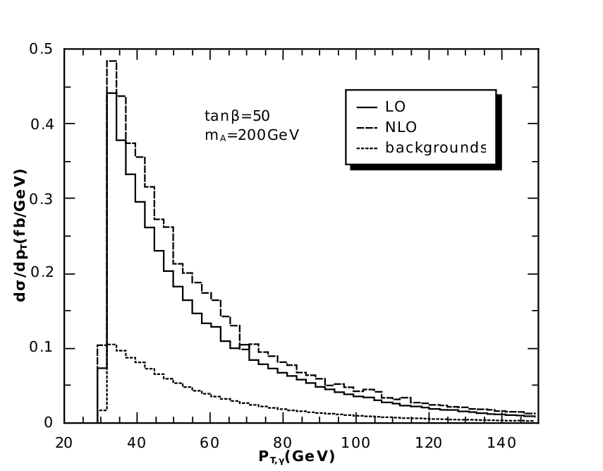
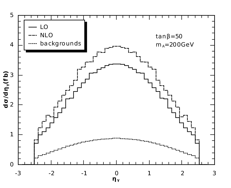
For the case of $m_{A}=200$ GeV in which a relatively large signal cross section and a high significance can be obtained, we investigate the NLO QCD effects more closely by studying various differential cross sections. Fig.14 shows the invariant mass distribution $d\sigma/dM_{\tau\tau}$ of the tau lepton pair. With the central region significantly enhanced by the NLO corrections, the mass peak for $A^{0}$ is clearly seen above the background. Fig.15 shows the photon transverse momentum distribution $d\sigma/dp_{T}^{\gamma}$ . The NLO QCD effects can enhance the LO results by as much as $13\%$ , depending on the specific value of $p_{T}^{\gamma}$ . Nevertheless, no significant distortion of the curve is found. In Fig.16, we present the photon pseudo-rapidity distribution $d\sigma/d\eta^{\gamma}$ together with the background. The NLO effects lead to moderate enhancement of the distribution, but do not change the shape of the curve either. Analysis of these differential cross sections shows that the NLO QCD corrections generally enhance the signature.

VI CONCLUSIONS

In conclusion, we have investigated the complete NLO QCD corrections to the inclusive total cross sections of $A^{0}\gamma$ associated production at the LHC in the MSSM. Our results show that the NLO corrections can enhance the total cross sections by $25\%\sim 15\%$ for Higgs mass $200$ GeV $<m_{A}<~500$ GeV and $\tan\beta=50$ . The SUSY QCD correction is negative and significant for light Higgs mass $m_{A}=200$ GeV, but is negligible for heavy Higgs mass $m_{A}=500$ GeV. The NLO corrections generally reduce the dependence of the total cross sections on the renormalization/factorization scale. Assuming a normal luminosity of $100$ fb^-1, we simulated the $\tau^{+}\tau^{-}+\gamma$ signature including the complete NLO QCD effects at the LHC, and found an observable signature above the SM background with a high signal significance in some regions of the MSSM parameter space allowed by the current experiments. Thus it can be expected that the LHC has the potential to discover a CP-odd Higgs boson with a mass of $200$ GeV $\sim 300$ GeV via the photon associated production channel for large $\tan\beta$ .

Acknowledgements.

This work was supported in part by the National Natural Science Foundation of China, under Grants No. 10721063, No. 10975004 and No. 10635030.

References

[1] F. Gianotti et al. Eur. Phys. J. C 39, 293 (2005).
[2] R. Barate et al. [LEP WG for Higgs boson searches], Phys. Lett. B 565, 61 (2003).
[3] S. P. Martin, A Supersymmetry Primer ,arXiv:hep-ph/9709356v5.
[4] J. R. Ellis et al., arXiv:0706.0977 [hep-ph].
[5] H. M. Georgi, S. L. Glashow, M. E. Machacek and D. V. Nanopoulos, Phys. Rev. Lett. 40, 692 (1978).
[6] M. Spira, A. Djouadi, D. Graudenz and P. M. Zerwas, Phys. Lett. B 318 (1993) 347; Nucl. Phys. B 453, 17 (1995).
[7] S. Dawson, A. Djouadi and M. Spira, Phys. Rev. Lett. 77, 16 (1996).
[8] A. Djouadi and M. Spira, Phys. Rev. D 62, 014004 (2000).
[9] R. V. Harlander and W. B. Kilgore, Phys. Rev. Lett. 88, 201801 (2002); JHEP 0210 017 (2002).
[10] C. Anastasiou and K. Melnikov, Nucl. Phys. B 646, 220 (2002); Phys. Rev. D 67, 037501 (2003).
[11] V. Ravindran, J. Smith and W. L. van Neerven, Nucl. Phys. B 665, 325 (2003).
[12] S. Catani, D. de Florian, M. Grazzini and P. Nason, JHEP 0307, 028 (2003).
[13] R. V. Harlander and M. Steinhauser, Phys. Lett. B 574, 258 (2003); Phys. Rev. D 68, 111701 (2003); JHEP 0409 066 (2004).
[14] A. Kulesza, G. Sterman and W. Vogelsang, Phys. Rev. D 69, 014012 (2004).
[15] R. N. Cahn and S. Dawson, Phys. Lett. B 136, 196 (1984).
[16] G. Altarelli, B. Mele and F. Pitolli, Nucl. Phys. B 287, 205 (1987).
[17] T. Han, G. Valencia and S. Willenbrock, Phys. Rev. Lett. 69, 3274 (1992).
[18] S. L. Glashow, D. V. Nanopoulos and A. Yildiz, Phys. Rev. D 18, 1724 (1978).
[19] R. Kleiss, Z. Kunszt and W. J. Stirling, Phys. Lett. B 253, 269 (1991).
[20] T. Han and S. Willenbrock, Phys. Lett. B 273, 167 (1991).
[21] S. Dawson, S. Dittmaier and M. Spira, Phys. Rev. D 58, 115012 (1998).
[22] T. Plehn, M. Spira and P. M. Zerwas, Nucl. Phys. B 479, 46 (1996); Nucl. Phys. B 531, 655(E) (1998).
[23] A. Belyaev, M. Drees, O. J. P. Eboli, J. K. Mizukoshi and S. F. Novaes, Phys. Rev. D 60, 075008 (1998).
[24] A. A. Barrientos Bendez and B. A. Kniehl, Phys. Rev. D 64, 035006 (2001).
[25] Z. Kunszt, Nucl. Phys. B 247, 339 (1984).
[26] W. Beenakker et al., Phys. Rev. Lett. 87, 201805 (1984); Nucl. Phys. B 653, 151 (2003).
[27] L. Reina and S. Dawson, Phys. Rev. Lett. 87, 201804 (2001).
[28] S. Dawson, L. H. Orr, L. Reina and D. Wackeroth, Phys. Rev. D 67, 071503 (2003).
[29] E. Gabrielli, B. Mele and J. Rathsman, Phys.Rev.D77, 015407 (2008), arXiv:0707.0797v2.
[30] K. Arnold, T. Figy, B. Jager, D. Zeppenfeld, arXiv:1006.4237v1.
[31] M. Chanowitz, M. Furman and I. Hinchliffe, Nucl. Phys. B 159, 225 (1979).
[32] Z. Bern, A. De Freitas, L. Dixon and H. L. Wong, Phys. Rev. D 66, 085002 (2002).
[33] I. Jack, D.R.T. Jones and K.L. Roberts, Z. Phys. C63, 151 (1994), arXiv:hep-ph/9401349.
[34] M. A. Aivazis et al., Phys. Rev. D 50, 3102 (1994).
[35] J. C. Collins, Phys. Rev. D 58, 094002 (1998).
[36] M. Kramer et al., Phys. Rev. D 62, 096007 (2000).
[37] D.A.Dicus and C.Kao, Phys. Rev. D 38, 1008 (1988) [Err.-ibid. D 42, 2412 (1990)].
[38] B. A. Kniehl, Phys. Rev. D 42, 2253 (1990).
[39] C. Kao, Phys. Rev. D 46, 4907 (1992).
[40] L. G. Jin, C. S. Li, Q. Li, J. J. Liu, R. J. Oakes, Phys.Rev. D71, 095004 (2005), arXiv:hep-ph/0501279v2.
[41] H. X. Zhu, C. S. Li, J. J. Zhang, H. Zhang, Z. Li, arXiv:0903.5047v2.
[42] A. Denner, Fortschr. Phys. 41 4 (1993).
[43] G. Passarino, M. Veltman, Nucl. Phys. B160 151 (1979).
[44] B. W. Harris, J. F. Owens, 10.1103/Phys.Rev.D 65, 094032 (2002), arXiv:hep-ph/0102128v3.
[45] J. C. Collins, D. E. Soper and G. Sterman, Nucl. Phys. B 261, 104 (1985).
[46] G. T. Bodwin, Phys. Rev. D 31, 2616 (1985); Phys. Rev. D 34, 3932 (E) (1986).
[47] S. Frixion, Phys. Lett. B429 369-374 (1998), arXiv:hep-ph/9801442; F. Stockli, A. G. Holzner, G. Dissertori, JHEP 0510, 079 (2005).
[48] E. Boos et al, [CompHEP Collaboration], CompHEP 4.4: Automatic computations from Lagrangians to events, Nucl. Instrum. Meth. A534 250 (2005) (arXiv:hep-ph/0403113).
[49] C. Amsler et al. (Particle Data Group), Physics Letters B 667, 1 (2008).
[50] M. Carena, D. Garcia, U. Nierste, C. E. M. Wagner, Nucl. Phys. B 577, 88 (2000).
[51] W. Porod, Comput. Phys. Commun. 153 275 (2003) (arXiv:hep-ph/0301101).
[52] B. C. Allanach et al, Eur. Phys. J. C25, 133 (2002).
[53] M. Drees and S. P. Martin, hep-ph/9504324.
[54] D. Stockinger, J. Phys. G 34, R45 (2007), hep-ph/0609168.

Next-to-leading order QCD predictions for A0​γA^{0}\gamma associated production at the CERN Large Hadron Collider

Abstract

pacs

I INTRODUCTION

II LEADING-ORDER CROSS SECTION FOR NEUTRAL HIGGS AND PHOTON ASSOCIATED PRODUCTION

III NLO QCD calculations

III.1 Virtual corrections

III.2 Real gluon emission

III.2.1 Hard non-collinear region

III.2.2 Soft region

III.2.3 Hard collinear region

III.3 Massless bottom (anti-)quark emission

III.4 Mass factorization

IV MONTE CARLO SIMULATION

V NUMERICAL RESULTS

V.1 NLO total cross section calculations

V.2 Simulation results

VI CONCLUSIONS

Acknowledgements.

References

Next-to-leading order QCD predictions for $A^{0}\gamma$ associated production at the CERN Large Hadron Collider