Astrometric search for a planet around VB 10Thanks: Based on observations made with ESO telescopes at the La Silla Paranal Observatory under programme ID 283.C-5024
Abstract
We observed VB 10 in August and September 2009 using the FORS2 camera of the VLT with the aim of measuring its astrometric motion and of probing the presence of the announced planet VB 10b. We used the published STEPS astrometric positions of VB 10 over a time-span of 9 years, which allowed us to compare the expected motion of VB 10 due to parallax and proper motion with the observed motion and to compute precise deviations. The achieved single-epoch precisions of our observations are about 0.1 mas and the data showed no significant residual trend, while the presence of the planet should have induced an apparent proper motion larger than 10 mas yr-1. Subtraction of the predicted orbital motion from the observed data produces a large trend in position residuals of VB 10. We estimated the probability that this trend is caused by random noise. Taking all the uncertainties into account and using Monte-Carlo resampling of the data, we are able to reject the existence of VB 10b with the announced mass of 6.4 MJ with the false alarm probability of only . A 3.2 MJ planet is also rejected with a false alarm probability of 0.023.
Key Words.
astrometry – technique: high angular resolution – planetary systems – stars: individual: VB 101 Introduction
The detection of a planetary-mass companion to the nearby M8 ultracool dwarf VB~10 (GJ~752B) was announced by Pravdo & Shaklan (2009). Using ground-based astrometric observations with the STEPS camera of the 5 m Palomar telescope obtained over nine years, the authors derived a full astrometric solution of the system that suggested the presence of a planetary companion with a 271 day orbital period and a 6.4 mass. Even though the VB~10b astrometric signature is large with a peak-to-peak value of 8 mas, the detection is debatable due to imperfect orbital sampling and comparably low astrometric accuracy of the individual measurements.
Zapatero Osorio et al. (2009) presented high-resolution near-infrared observations of VB 10 obtained between 2001 and 2008 with the NIRSPEC instrument on the Keck II telescope. They emphasized on the necessity to have a better sampling of the orbital phase to precisely constrain the orbital parameters and the individual masses of the system. Bean et al. (2010) used the near-infrared CRIRES spectrograph and did not detect the planet’s signature in radial-velocity (RV). Anglada-Escudé et al. (2010) performed a joint analysis of precise RV observations over 175 days with MIKE/Magellan and ESPaDOnS/CFHT spectrographs, RV measurements by Zapatero Osorio et al. (2009), and astrometric data by Pravdo & Shaklan (2009). They showed that the observed astrometric motion is not due to an unseen companion.
We present results of the astrometric search for the planet using the FORS2 camera of the VLT, the only instrument which can achieve astrometric precision of individual measurements of 0.05–0.1 mas (Lazorenko et al., 2009). Despite the short observation period of two months, we obtained data sufficiently good to verify the hypothesis on the possible existence of VB 10b.
2 Observations
Observations were made with the FORS2/VLT camera (Appenzeller et al., 1998) in imaging mode during five nights from 2 August to 25 September 2010. The images cover a ′field of view with a pixel (px) scale of 0.1″/px. For each night, we obtained 21 to 72 frames of 7 s exposures with the filter. Seeing varied from 0.55″to 0.9″. To reduce differential chromatic refraction (DCR) of the atmosphere, observations were made near meridian.
Because the observed motion of VB 10 in the sky is large (over 2 px), we had to know the precise pixel scale to convert pixel to arcsec units without loss of accuracy. From CMC14 and NOMAD catalogue positions of stars in our reference frame, we derived acceptably precise scales of ″/px and ″/px in RA and Decl, respectively.
3 Data reduction and analysis
Our null hypothesis was that the planet VB 10b exists. To test this hypothesis, we computed the residuals of our measurements compared to the position of VB 10 expected from the combination of proper, parallactic, and orbital motions. By determining the probability that the measured residuals are compatible with the expected mean value of zero, we could confirm or reject the null hypothesis. We also performed the corresponding computations assuming that the planet does not exist.
In all cases, we considered that the astrometric signal in VB 10 position induced by the planet is defined by the orbital elements of VB 10b given in the discovery paper by Pravdo & Shaklan (2009). The predicted orbital motion over the measurement timespans of 17 and 54 days is 0.48 and 1.95 mas in RA and 0.92 and 3.28 mas in Decl, respectively. Compared to the astrometric precision of FORS2 of about 0.1 mas per epoch, these displacements are large and should be detected in this study.
3.1 Photocentre determination
Raw images were flat-fielded and bias-subtracted to exclude pixel-to-pixel variations of the CCD sensitivity. To increase the number of reference stars, we measured all star images with –21. At this faint end, the star field is very crowded. This forced us to improve our procedure of photocentre computation, which initially was developed for isolated stellar images (Lazorenko, 2006). We scanned images obtained under various seeing conditions and made a detailed census of star positions at subpixel precision, of fluxes, and of the point-spread function variation across the CCD. This information was used to accurately model and subsequently subtract the contamination of background counts caused by distant stars. Wings of star profiles at distances up to 50 px were approximated by exponential function with free parameters smoothly varying over the CCD. The photocentres and were computed by fitting star profiles in a px window with a model with 12 free parameters and an auxiliary oscillating function in the central px window (Lazorenko, 2006). Computations based on the Levenberg-Marquardt numerical algorithm of the least squares fit were found to give sufficiently good results for stars of approximately equal brightnesses at separations larger than about 10 px.
3.2 Astrometric model
Reductions were based on the method previously applied to FORS1/2 observations (Lazorenko et al., 2007; Lazorenko et al., 2009). The method was shown to efficiently mitigate atmospheric image motion, geometric field distortion, DCR, and other effects, thus ensuring precision stable over time scales of a few days to a few years. For every star in the field, i.e. VB 10 and the reference stars, the measured photocenter positions and in frame at time were represented by the model
| (1) |
The left side contains the free model parameters and the model function . The expression for -data is similar but contains instead of . Here, is a zero point, is the mode (arbitrary even integer, usually from 4 to 16), is a polynomial in and of order that models the sum of atmospheric image motion and geometric distortion for each frame . The parameter is the proper motion, is the parallax, and is the parallax factor in . The displacement of the star image due to DCR is modelled by a term with leading parameter , which depends on the star’s colour, and containing the zenith distance and the angle between a direction to zenith and -axis. The next term describes an image displacement opposite to that of DCR and introduced by the longitudinal atmospheric dispersion compensator (LADC) of the VLT (Avila et al., 1997). This displacement also depends on the star colour via the parameter . Both and are free model parameters and their computation does not require external colour data. The LADC is automatically adjusted to the average zenith distance over a given series of frames by setting a distance between its two prisms to . Finally, represents the induced orbital motion of VB 10 if the planet exists. For reference stars, .
Equation 1 defines a system of equations in the combined {, , }-domain for which the unique solution is derived under the condition that the model parameters of reference stars are orthogonal to each basic function of . It is solved iteratively for all reference stars available in a circular region of radius which increases with and is centered on the target VB 10. The optimal field size is the size at which the noise from a reference field is equal to the noise from atmospheric image motion. The number of reference stars depending on varies from a few dozens to 500. Due to the large number of reference stars, the function accurately reproduces the coordinate grid distortion introduced by image motion. Solutions for at each mode are then used to form equations for the target in the time domain only. The solution of this new set of equations yields the target’s model parameters and position deviations from the model. The final output is the average obtained from the solutions at all modes .
 |
 |
 |
3.3 Comparison of STEPS and FORS2 reference frames
Because of different zero-points, STEPS proper motion cannot be directly applied to FORS2 astrometry. The STEPS reference frame is given by 15 bright stars. For the FORS2 reference frame, we use both these (except STEPS star Nr. 10 which is a binary) and a number of much fainter stars. The system of proper motions is defined under the condition where summation is taken over all reference stars with weights approximately proportional to their brightness (Lazorenko et al., 2009). In particular, this condition is valid for the proper motions of the STEPS stars which, due to their high brigthness (they contribute to over 40% of the total light flux), are the basis of the FORS2 reference frame. Hence, one may expect that (the weighted mean proper motion in the system of FORS2 proper motions) taken over these stars, is nearly zero. The computed value of this sum (which is the difference of proper motion zero-points) was found to be small: and mas yr-1 in RA and Decl. Due to the low precision, we did not apply it but included it in the error budget assuming that the uncertainty in the proper motion zero point is 1 mas yr-1. Thus, both proper motion systems are well consistent, however at time scales of yr only.
3.4 Short and full dataset
The data reduction of the first epoch (2 Aug) was problematic because of incorrect telescope pointing, owing to which all stars in a 300 px wide area just below VB 10 (Fig. 1a) were imaged to another CCD chip and could not serve as reference at this particular night. We dealt with this problem in two ways. In the first version, we put aside all stars within this area from frames of all nights, using only stars outside of this area as reference objects. The sizes and shapes of the reference fields in this case are shown in Fig. 1a by five circular segments, each corresponding to increasing from six (small radius) to 14 (large radius). Alternatively, we used circular reference areas, which for the 2 Aug night were of the same size but with the lower half vignetted (Fig. 1b). We also examined a short dataset without the 2 Aug epoch with circular reference area (Fig. 1c). The asymmetry of the first two cases degraded the obtained precision in comparison to the symmetric configurations of the short dataset.
We have obtained a solution for all three cases presented in Fig. 1. For the final result, we present two solutions. One is obtained from the short dataset (case ’c’, MJD between 55082 and 55099 days), and the second one is obtained as the average of the results in case ’a’ and ’b’. The latter solution is referred to as obtained from the full dataset (MJD between 55045 and 55099 days).
3.5 Recovering LADC positions
VB 10 is very red and differs much in colour from the reference stars. Therefore, the DCR displacement of this star is very large and about 30 mas in Decl and 10 mas in RA. This is taken into account by the free model parameters and , but their adjustment requires knowledge of the LADC separation .

Information on was not part of the obtained fits headers and was not accessible to us. Therefore we had to solve the inverse problem of recovering LADC separations from the observations. Because is fixed for a series of frames of a single night, we had to determine a small number of values for b (one value per night). Our approach is based on the observation that incorrect values of bias the average night position residuals and of field stars. According to Eq. 1, this bias linearly depends on the star colour parameter during one given night. This is illustrated by Fig. 2 which shows the distribution and linear dependencies of on for field stars in the case of the short dataset (the effect is largest in ).
Because all observations were made at small hour angles within 0.7 h, we initially assumed that LADC was always set to the separation corresponding to the meridian. By applying small corrections to these initial values of , we iteratively reached a solution without dependence of on colours (lower panel of Fig. 2). For these computations, we used all stars within the entire field of view of FORS2, processing them as target objects relative to their own subsets of reference stars. Being based on field stars only, this procedure produced a much smaller dispersion of values for VB 10 and for reference stars with large colours. Corrections to were small and within % of the initial values and were found with precision corresponding to mas error in for VB 10. For the full dataset, precision degraded to mas because we could not use stars in the problematic 300 px area below VB 10 (Fig. 1a).
3.6 Treatment of colour-dependent terms
An essential drawback of the above procedure is that the recovery of introduces small colour-dependent terms and , which are similar to proper motion and parallax. This is because the above iterations do not garantee convergence to the actual values of . For example, the restored value of may differ from its actual value by a term which progressively changes in time as , where is an arbitrary constant and is the average value of during the given night. Hence the term in Eq. 1 generates the term linearly dependent on and which therefore can be treated as an extra image motion . The term compensates for the linear change of in time. Similarly, we may assume that the restored values of contain terms proportional to and . In this case, the solution of Eq. 1 for parallax should contain the compensating colour-dependent term .
When recovering values, we cannot control the amplitude of and of the equivalent parameter related to parallax. However, they can be detected as proper motion and parallax dependence on colours (i.e. on ) which we model as a linear trend in proper motions of field stars and statistically correct for it.
The strong correlation between , , and does not allow us to determine separately and . However, this is not required because for short times , we can approximate the sum of the proper motion and parallax displacement by , where is the new effective quantity that substitutes for both and . Thus processing the short dataset, we find and use only a single colour term . The treatment is similar for the components. Subtraction of from the measured positions thus simultaneously eliminates the colour term (see next section). The value of this correction for VB 10 in Decl is mas yr-1 for the full and mas yr-1 for the short dataset, respectively. In RA, the corrections are an order of magnitude smaller.
For the full dataset, the above approximation of by is still valid for reference stars, most of which have moderate and therefore very small colour-induced parallaxes . But it is not sufficiently precise for VB 10, because of its large colour term . Consequently, is not accurately eliminated by applying the correction as in the case of the short dataset. Therefore, we had to treat the term of VB 10 as a free model parameter.

3.7 Subtraction of parallax and proper motions
Since the FORS2 observations cover a small fraction ( %) of the orbital period, can be approximated as a linear function of :
| (2) |
where and . With the orbital elements given by Pravdo & Shaklan (2009), we obtained and mas yr-1 (Fig. 3). Astrometric acceleration terms (deviations from the linearity) are smaller than mas for the full dataset, thus are negligible. For the short dataset, they are even smaller than 0.02 mas.
In addition, is approximately a linear function of the parallax factors and , which themselves have an approximately linear time-dependence. This causes a strong correlation between parallax, proper motion, and orbital motion, thus makes Eq. 1 degenerated. Therefore, we subtracted parallax and proper motion from the measured positions of VB 10. Precise values of these parameters were found based on the published STEPS astrometric measurements which cover a 9 years long period. The best fit of STEPS data yielded mas yr-1, mas yr-1, and mas. These values are very close to the estimates given by Pravdo & Shaklan (2009) and Anglada-Escudé et al. (2010).
 |
 |
 |
3.8 Position residuals of models with and without planet
Subtracting the contributions of parallax and proper motion from the measured positions of VB 10 resulted in great simplification of Eq. 1, which for VB 10 took the form
| (3) |
with only four free parameters , , , and in the case of the short dataset. For the full dataset, it incorporates the extra parameter (the term in curly braces, see Sect. 3.6). The right side of Eq. 3 contains the measured coordinates and , the in-plate solutions and derived from the reference stars, and all other corrections.
There is a correlation between the orbital signal and the night average angles which are not zero and tend to increase in time. Because of this correlation, the model Eq. 1 filters out any component of the signal (e.g. ), which is linearly dependent on and enters the right side of Eq. 1. Therefore, the output position residuals contain only a part of the initial signal amplitude. However, this does not hamper our statistical analysis, which we performed after the subtraction of from the observed positions, thus assuming zero input signal and consequently zero output signal. In this way, the impact of correlations is minimized. If the planet does not exist but the subtraction of was applied, we should detect the inverse signal reduced in amplitude because of the correlation between and . This is the case corresponding to the last row of Table 2 (Sect. 4), where the measured signal (expressed by the parameter ) has about half its expected value (PS).
Fig. 4 shows the results in terms of model deviations in Decl, where the expected signal is largest. The single-frame precision includes errors of photocentre measurements, the reference frame noise, and the atmospheric noise. It varies from 0.4 to 0.7 mas depending on seeing. The effect of the vignetted reference field of the 2 Aug epoch (configurations ’a’ and ’b’) is seen as a degradation of to over 1 mas. At other epochs, is larger compared to configuration ’c’ because of a larger .
Clear conclusions can be drawn from the short dataset when the model (Eq. 3) is most simple and does not require incorporation of parallax (Sect. 3.6). We considered the cases with the predicted orbital motion subtracted () and with . The epoch average deviations and are very small and randomly scattered when assuming , but display a negative trend in time if . Note that small position deviations do not correspond to a ’zero’ measurement. Instead, they demonstrate very precise position measurements, which track the proper motion and parallax displacement at the daily rate of 2.7 mas and 5.0 mas in RA and Decl, respectively. The motion of VB 10 over the CCD surface (Fig. 5) for the measurement timespans of 17 days is 46 mas in RA and 86 mas in Decl, and is dominated by parallax and proper motion. DCR effects induce a small-scale scatter in the measured positions of one night with an amplitude of about 2 mas. Their structure for a typical night is shown in 5-fold magnification in Fig. 5.

Similar computations were performed for the full dataset, where we had to account for the parallax correction (see Sect. 3.6), thus used the five parameters , , , , and for fitting of the model Eq. 3. This introduced a strong correlation between , , and , which reduced the amplitude of the detected signal.
| MJD | RA | Decl | RA | Decl | |||
| 55000+ | (mas) | (mas) | (mas) | (mas) | (mas) | (mas) | (mas) |
| Full dataset, 2 Aug–25 Sept 2009 | |||||||
| 45.163 | -0.26 | -0.16 | -0.79 | 0.41 | 0.19 | 0.64 | 0.32 |
| 82.032 | 0.20 | 0.19 | 0.15 | 0.35 | 0.10 | 0.18 | 0.16 |
| 92.993 | -0.09 | -0.06 | -0.06 | 0.11 | 0.08 | 0.11 | 0.10 |
| 97.014 | -0.00 | 0.18 | 0.03 | 0.08 | 0.07 | 0.11 | 0.09 |
| 99.011 | -0.01 | -0.25 | 0.03 | -0.38 | 0.07 | 0.12 | 0.10 |
| Short dataset, 8–25 Sept 2009 | |||||||
| 82.032 | 0.07 | -0.09 | 0.33 | 0.43 | 0.11 | 0.19 | 0.16 |
| 92.993 | -0.02 | -0.04 | -0.12 | -0.09 | 0.09 | 0.09 | 0.06 |
| 97.014 | 0.03 | 0.07 | 0.02 | -0.00 | 0.07 | 0.08 | 0.05 |
| 99.011 | -0.06 | -0.01 | -0.09 | -0.15 | 0.08 | 0.09 | 0.07 |
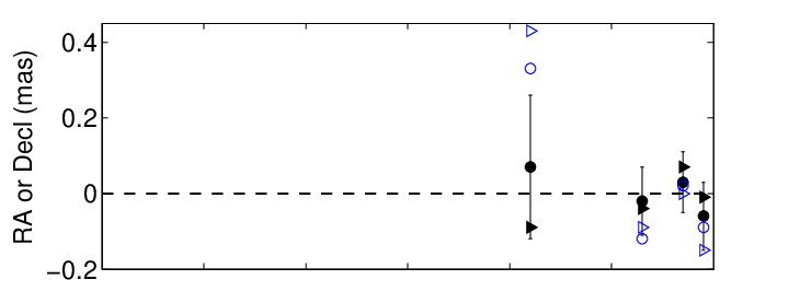
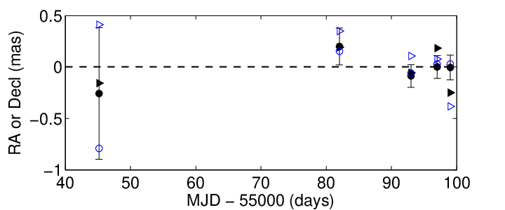
Table 1 and Fig. 6 summarise the results for the epoch residuals and . The astrometric precision is described by a nominal precision based on errors in photocentre determination, the reference frame noise and atmospheric noise. also includes error components which dominate at long time spans and originate from the uncertainties in , , pixel scale, and proper motion of VB 10. For the full dataset, it also includes the uncertainty in the parallax of VB 10. is the mathematical expectation of the root-mean-square of and , derived from the least squares fit (Eq. 3).
 |
 |
4 Discussion
Because the signal was subtracted in Eq. 3, the epoch deviations and should have an expectation value of zero and a random scatter irrespective of the model (with or without planet). A small dispersion of and values indicates that the tested hypothesis is correct. The data shown in Fig. 6 and Table 1 is more consistent with (the hypothesis of no planetary companion), while incorporating a non-zero planetary signal increases the scatter of data points, which does not support the existence of the planet VB 10b. We estimated the probability that the planet exists in two ways.
The first estimate was based on the values of , where the sum is taken over epochs. The number of degrees of freedom (D.o.F.) is equal to the number of epochs minus the number of model parameters (there are two and three free parameters for the short and the full dataset, respectively). The probabilities corresponding to the values are given in Table 2. For both the short and the full dataset, they are at the equally small at the 2% level if the model assumes . Because the probability of this event is low, the large scatter of and is unlikely to be caused by random noise in the observations.
| Dataset | D.o.F. | ||||||
|---|---|---|---|---|---|---|---|
| full | 0 | 10.6 | 7 | 0.16 | 0.67 | -0.35 | 0.36 |
| full | 18.0 | 7 | 0.02 | 4.14 | -5.38 | 0.02 | |
| short | 0 | 1.9 | 6 | 0.93 | -2.06 | 2.47 | 0.21 |
| short | 14.8 | 6 | 0.02 | -7.82 | -11.32 |
Secondly, we noticed that the observed residuals and show a linear trend instead of a random distribution. This can be caused by random errors in the observations, but also may indicate a wrong value of the signal subtracted in Eq. 3. In the latter case, we would expect that the residuals and show a linear dependence opposite to (see Eq. 2).
A large negative trend is seen for the short dataset residuals computed with (Fig. 6), whereas they should be near zero to support the planetary hypothesis. In contrast, a much smaller trend is observed when assuming (no planet). For instance, the measured values of given in Table 2 for the short dataset and are -7.82 and -11.32 mas yr-1 in RA and Decl, respectively. If the null hypothesis is correct, their expected values are 0 and 0 mas yr-1, and -13.4 and -22.4 mas yr-1 if the hypothesis is wrong (). In the last case, the measured values are always smaller than the values induced by the orbital motion, because their magnitude is damped by correlations between and model parameters (cf. Sect. 3.8).
Because the criterion is not the most efficient one for the characterisation of linear signals, we developed another, more powerful approach to obtain an alternative estimate of . We considered as quantities describing the dispersion of and better than and performed Monte Carlo simulations to see if the observed features can be explained by random noise in the observations. We simulated each data frame by a random Gaussian noise with root-mean-square of and added components modelling the errors in , , and in the proper motion and parallax of VB 10. In addition, we included a 1 mas yr-1 error to account for the uncertainties in the zero point of proper motion (cf. Sect. 3.3).
After fitting the data with the model Eq. 3, we searched the residuals for linear trends in time and estimated their coefficients . The false-alarm probabilities that a random noise produces values larger than the observed ones are given in Table 2. In the case of the short dataset and , we find that the observed linear trends can be explained by Gaussian noise with a probability of , which does not support the existence of the planet. For the full dataset, we find , which is not sufficient to draw definite conclusions. In spite of the longer timespan and therefore seemingly better conditions to characterise a planetary signal, the full dataset does not provide a better contraint because of the uncertainty in , whose contribution increases with time. Besides, the planetary signal is substantially damped because of its strong correlation with the colour correction used in Eq. (3) as a free model parameter.
5 Conclusions
We conclude that the presence of the announced planet around VB 10 is not supported by astrometry. Even assuming half the planetary mass (i.e. 3.2 MJ), simulations give a low false alarm probability , which does still not support the existence of VB 10b. Our result obtained from astrometry alone is in agreement with the conclusion of Bean et al. (2010) and Anglada-Escudé et al. (2010) based on RV data.
This study is the first application of the FORS2 camera for the search of exoplanets by means of optical astrometry. Because of the high astrometric precision of FORS2, the availability of external STEPS-based proper motion and parallax of VB 10, and the large expected orbital signal, it was possible to perform the verification of the planetary companion hypothesis within the extremely short observation period of 17 days, which is unusual for astrometric works of this type. The successful use of the STEPS data for the reduction of FORS2 observations is justified only because we verified that the STEPS and FORS2 proper motion reference frames are consistent within 1 mas yr-1 uncertainty.
We have demonstrated a mean nominal precision of 0.09 mas per epoch of FORS2/VLT observation for data of reasonable quality, despite problems caused by the uncertainty in the LADC position. This precision is sufficient for astrometric detection of planets around ultracool dwarfs.
Acknowledgements.
We thank Dr. G. Anglada-Escudé whose comments have helped to improve the paper. PF and NCS would like to thank the support by the European Research Council/European Community under the FP7 through a Starting Grant, as well as the support from Fundação para a Ciência e a Tecnologia (FCT), Portugal, in the form of a grant with reference PTDC/CTE-AST/098528/2008. NCS would further like to thank the support from Fundação para a Ciência e a Tecnologia (FCT), Portugal, through a Ciência 2007 contractfunded by FCT/MCTES (Portugal) and POPH/FSE (EC).References
- Anglada-Escudé et al. (2010) Anglada-Escudé, G., Shkolnik, E. L., Weinberger, A. J., et al. 2010, ApJ, 711, L24
- Appenzeller et al. (1998) Appenzeller, I., Fricke, K., Fürtig, W., et al. 1998, The Messenger, 94, 1
- Avila et al. (1997) Avila, G., Rupprecht, G., & Beckers, J. M. 1997, in SPIE, Vol. 2871
- Bean et al. (2010) Bean, J. L., Seifahrt, A., Hartman, H., et al. 2010, ApJ, 711, L19
- Lazorenko (2006) Lazorenko, P. F. 2006, A&A, 449, 1271
- Lazorenko et al. (2007) Lazorenko, P. F., Mayor, M., Dominik, M., et al. 2007, A&A, 471, 1057
- Lazorenko et al. (2009) Lazorenko, P. F., Mayor, M., Dominik, M., et al. 2009, A&A, 505, 903
- Pravdo & Shaklan (2009) Pravdo, S. H. & Shaklan, S. B. 2009, ApJ, 700, 623
- Zapatero Osorio et al. (2009) Zapatero Osorio, M. R., Martín, E. L., del Burgo, C., et al. 2009, A&A, 505, L5