Multiscale Gossip for Efficient Decentralized Averaging in Wireless Packet Networks
Abstract
This paper describes and analyzes a hierarchical algorithm called Multiscale Gossip for solving the distributed average consensus problem in wireless sensor networks. The algorithm proceeds by recursively partitioning a given network into subnetworks. Initially, nodes at the finest scale gossip to compute local averages. Then, using multi-hop communication and geographic routing to enable gossip between nodes that are not directly connected, these local averages are progressively fused up the hierarchy until the global average is computed. We show that the proposed hierarchical scheme with levels of hierarchy is competitive with state-of-the-art randomized gossip algorithms in terms of message complexity, achieving -accuracy with high probability after messages. Key to our analysis is the way in which the network is recursively partitioned. We find that the optimal scaling law is achieved when subnetworks at scale contain nodes; then the message complexity at any individual scale is . Another important consequence of hierarchical construction is that the longest distance over which messages are exchanged is hops (at the highest scale), and most messages (at lower scales) travel shorter distances. In networks that use link-level acknowledgements, this results in less congestion and resource usage by reducing message retransmissions. Simulations illustrate that the proposed scheme is more message-efficient than existing state-of-the-art randomized gossip algorithms based on averaging along paths.
I Introduction
Distributed signal and information processing applications arise in a variety of contexts including wireless sensor networks, the smart-grid, large-scale unmanned surveillance, and mobile social networks. Large-scale applications demand protocols and algorithms that are robust, fault-tolerant, and scalable. Energy-efficiency is also an increasingly important design factor. When a system is comprised of battery-powered nodes or agents equipped with wireless radios for transmission—such as in wireless sensor networks—energy-efficiency equates to requiring few transmissions since in addition to consuming bandwidth, each wireless transmission dissipates battery resources.
Gossip algorithms [2, 3, 4, 5, 6] are an attractive paradigm for decentralized, in-network processing, and have received much attention in the computer science, systems and control, information theory, and signal processing research communities of late. Gossip algorithms are frequently posed and studied as solutions to the distributed averaging problem: in a network of nodes whose topology is described by a graph with , each node initially has a scalar value , and the goal is to approximate the average, at every node. Nodes iteratively and asynchronously exchange estimates with a small subset of the entire network, updating their local estimate after each exchange. These protocols have a number of attractive properties. The simplicity of the protocol (exchange information, update, repeat) makes it extremely robust; since there is no fixed routing of information to a fusion center and since all nodes compute a solution, there is no single point of failure or bottleneck. Furthermore, past studies have demonstrated that gossip algorithms converge even under unreliable or dynamic networking conditions; see, e.g., [6] and references therein.
However, the standard gossip algorithms for distributed averaging [2, 3, 4, 5] constrain information to only be exchanged between neighboring nodes and exhibit poor scaling and energy-efficiency in topologies frequently used to model connectivity in wireless networks, such as grids and random geometric graphs [7]. Roughly speaking, the number of messages transmitted per node depends linearly on , the size of the network. Since the values required to compute the average are initially stored at different nodes, any distributed averaging algorithm requires that each node perform at least one transmission. This discrepancy between constant and linear transmissions per node, has motivated the development of a number of variants of gossip algorithms specifically aimed at improving the efficiency of gossip on grid and random geometric graph topologies (see Section II for more).
The principle of hierarchical (multiscale) decomposition, or divide-and-conquer, arises in a variety of settings as a mechanism which yields efficient information processing procedures. In the signal processing and coding communities, multiscale analysis is frequently associated with wavelet-based methods, e.g., for signal and image denoising, edge detection, and transform coding [8]. A hierarchical approach to communication over wireless networks was shown to achieve the optimal capacity scaling law [9]. A recent study also found that flocks of birds exhibit hierarchical organization and suggested that hierarchical behavior has been selected (in the evolutionary sense) because it is more efficient than democratic or individualistic strategies [10].
This paper describes and analyzes a multiscale gossip algorithm for distributed averaging in grid and random geometric graph topologies. The network is recursively partitioned into smaller subnetworks. The size of subnetworks at each scale and the number of scales of the partition depend on the number of nodes in the network. Multiscale gossip operates over this partition in a bottom-up fashion. First, all nodes within each subnetwork at the finest scale gossip until computing a suitably accurate local average. Then, a representative node is elected for each subnetwork; an overlay grid is formed among all representatives within the same subnetwork at the next higher scale, and the representatives gossip over the overlay grid. This procedure is repeated until representatives at the coarsest scale have computed an accurate approximation to the network average. At that point the representatives disseminate their estimate to all of their children in the hierarchy. Multi-hop communication between representatives at coarser scales is accomplished using geographic routing [11, 12].
Our main contribution is the analysis of multiscale gossip. In particular, for a carefully designed multiscale partition, we show that the total number of single-hop transmissions required to reach a desired level of accuracy scales nearly-linearly, requiring total transmissions as on random geometric graph and grid topologies. Consequently, the average number of transmissions per node is . Since information dissemination (randomized broadcast) is much more efficient than gossip (which is a form of information diffusion) in these topologies, representatives at all scales can optionally disseminate intermediate results to other nodes in their subnetwork, thereby improving robustness and fault-tolerance of the scheme, without affecting the order-wise scaling law. In contrast to geographic gossip with path averaging [13], a randomized gossip scheme with a linear scaling that also uses geographic routing to exchange information over multiple hops, multiscale gossip requires fewer and shorter multi-hop transmissions; for example, in a grid topology, path averaging requires relaying messages over hops, whereas multiscale gossip messages at the coarsest scale are relayed over at most hops, and messages at finer scales travel significantly shorter distances. This has advantages when reliable transmission (i.e., handshaking, forward error-correcting, and/or retransmission) protocols are used at the link-level to ensure accurate reception over each link of a multi-hop path. Moreover, at each iteration of multiscale gossip, information is only exchanged between one pair of nodes, as opposed to all nodes along a path.
The remainder of this paper is organized as follows. Section II covers background, and related work. Section III describes the procedure for recursively constructing the hierarchical network partition and for carrying out multiscale gossip. Then, our main results are presented in Section IV, with analysis and proofs provided in Section V. A numerical evaluation of the proposed algorithm is presented in Section VI. Some practical considerations are discussed in Section VII, and we conclude in Section VIII.
II Background and Problem Definition
Our primary measure of performance is communication cost—the number of messages (single hop transmissions) required to compute an estimate to accuracy—which is also considered in [11, 13]. Moreover, we are interested in characterizing scaling laws, or the rate at which the communication cost increases as a function of network size. In the analysis of scaling laws for gossip algorithms, a commonly studied measure of convergence rate is the -averaging time, denoted and defined as [2]
| (1) |
which is the number of iterations required to reach an estimate with accuracy with high probability. The -averaging time reflects the idea that the complexity of gossiping on a particular class of network topologies should depend both on the final accuracy and the network size. When only neighbouring nodes communicate at each iteration, and communication cost are identical up to a constant factor. Otherwise, communication cost can generally be bounded by the product of and a bound on the number of messages required per iteration.
In wireless sensor network applications, random geometric graphs are a typical model for connectivity since communication is restricted to nearby nodes. In the -dimensional random geometric graph model, nodes are randomly assigned coordinates uniformly in the unit square, and two nodes are connected with an edge when their Euclidean distance is less than or equal to a connectivity radius, [7, 14]. In [7] it is shown that if the connectivity radius scales as then the network is connected with high probability. Throughout this paper when we refer to a random geometric graph, we mean one with the connectivity .
Although the standard neighbor gossip algorithms are known to be efficient on complete graphs and expander-like topologies, they are also known to converge slowly on grids and random geometric graphs, two topologies commonly used to model wireless networks [3, 2]. Kempe, Dobra, and Gehrke [3] initiated the study of scaling laws for gossip algorithms and showed that gossip requires total messages to converge on complete graphs. Boyd, Ghosh, Prabhakar, and Shah [2] studied scaling laws for standard randomized gossip on random geometric graphs and found that communication cost scales as messages even if the algorithm is optimized with respect to the topology. This finding motivated the pursuit of efficient gossip algorithms for wireless networks in a number of interesting directions. For a complete overview of this line of work, we refer the reader to the recent survey [6]. Here we briefly discuss different approaches, focusing on advances most closely related to the present article.
A number of approaches seek more efficient computation while enforcing the constraint that information only be exchanged between neighboring nodes at each iteration. Most of these approaches introduce memory at each node, creating higher-order updates similar to shift-registers or polynomial filters [15, 16]. Scaling laws for a deterministic, synchronous variant of this approach are presented in [17], leading to communication cost. Related asynchronous gossip algorithms based on lifted Markov chains have been proposed that achieve similar scaling laws [18, 19]. Recent work [20] suggests that no gossip algorithm on grids and random geometric graphs can achieve better than scaling while constraining information exchange to be solely between neighboring nodes.
A variant called geographic gossip, proposed by Dimakis, Sarwate, and Wainwright [11], achieves a communication cost of by allowing distant (non-neighbouring) pairs of nodes to gossip at each iteration. Assuming that each node knows its own coordinates and the coordinates of its neighbours in the unit square, communication between arbitrary pairs of nodes is made possible using greedy geographic routing. Rather than addressing nodes directly, a message is sent to a randomly chosen target -location, and the recipient of the message is the node closest to that target. To reach the target, a message is forwarded from a node to its neighbour who is closest to the target. If a node is closer to the target than all of its neighbours, this is the final message recipient. It is shown in [11] that for random geometric graphs with connectivity radius , greedy geographic routing succeeds with high probability. For an alternative form of greedy geographic routing, which may be useful in implementations see [12]. The main contribution of [11] is to illustrate that allowing nodes to gossip over multiple hops can lead to significant improvements in message cost. In follow-up work, Benezit, Dimakis, Thiran, and Vetterli [13] showed that a modified version of geographic gossip, called path averaging, can achieve message cost on random geometric graphs. To do this, all nodes along the path from the source to the target participate in a gossip iteration. If geographic routing finds a path through nodes to deliver a message from to , the estimates of all nodes in are accumulated on the way to . Then computes the average of all values and sends the average back down the same path towards , and all nodes in update their estimates.
Observe that there is a tradeoff between algorithmic simplicity and performance. If we only allow pairwise communication between neighboring nodes, we cannot beat the barrier. On the other hand, if we have the additional knowledge of geographical information for each node and its immediate neighbours, we can use geographic routing and with the added complexity of averaging over paths we can bring the message complexity down to linear at the expense of messages having to travel potentially over hops. However, in order to improve upon the performance achievable using pairwise communication between neighboring nodes, some additional complexity must be introduced. In this work, rather than averaging along paths, we propose to decompose computation in a multiscale manner in order to achieve faster convergence.
The multiscale approach considered in this paper also assumes that the nodes know their own and their neighbour’s coordinates in the unit square. Using the geographic information, we derive a hierarchical algorithm that asymptotically achieves a communication cost of messages, which is equivalent to that of path averaging up to a logarithmic factor. However, in multiscale gossip, information is only exchanged between pairs of nodes, and there is no averaging along paths. At the expense of extra complexity for building the logical hierarchy, besides near-optimal communication cost we achieve two other important goals. First, the longest distance a message travels in our multiscale approach is hops which is much shorter compared to hops for geographic gossip or path averaging. This can prove significant if an adversary wishes to disrupt gossip computation by forcing the network to drop a particular message or by deactivating a node in the middle of an iteration. In that scanario a substantial amount of information can be lost in path averaging since each iteration involves nodes on average. Second, as we show later on, multiscale gossip distributes the computation quite evenly across the network and does not overwhelm and deplete the nodes located closer to the center of the unit square as is the case for path averaging.
We note that we are not the first to propose gossiping in a multiscale or hierarchical manner. Sarkar et al. [21] describe a hierarchical approach for computing aggregates, including the average. However, because their algorithm uses order and duplicate insensitive synopses to estimate the desired aggregate, the size of each message exchanged between a pair of nodes must scale with the size of the network. Other hierarchical distributed averaging schemes that have been proposed in the literature focus on the synchronous form of gossip, and they do not prove scaling laws for communication cost, nor do they provide rules for forming the hierarchy (i.e. assume the hierarchical decomposition is given) [22, 23, 24]. Finally, we mention that hierarchical approaches to routing have also been proposed [25, 26]. Although this line of work uses similar techniques (hierarchy and divide-and-conquer approach) the problems considered are not related to distributed averaging.
A preliminary version of this work appears in the conference paper [1] where multiscale gossip is described, including our construction of the multiscale network partition and a simple communication cost analysis. The present manuscript extends [1] in several ways. In addition to more detailed communication cost analysis, the proof of the final error bound of multiscale gossip is a new result. Moreover, we investigate the role of the subdivision parameter , explaining in what sense the value is optimal. Finally, we include a thorough set of experiments to evaluate the performance of multiscale gossip.
III Multiscale Gossip
Multiscale gossip performs averaging in a hierarchical manner. At each moment only nodes in the same level of hierarchy do computations at a local scale and computation at one level begins after the previous level has finished. By hierarchically decomposing the initial graph into subgraphs, we impose an order in the computation. As shown in the next section, for a specific decomposition it is possible to divide the overall work into a small number of linear sub-problems and thus obtain very close to linear complexity in the size of the network.

Assume we have a random geometric graph and each node knows its own coordinates in the unit square and the locations of its immediate neighbours. Each node also knows the total number of nodes in the network and , the desired number of hierarchy levels11 1 As explained in Section V, given , the number of levels can be computed automatically.. Figure 1 illustrates an example with . We use the convention that level is the lowest level where the unit square is split into many small cells. Level is the top level where we only have few big cells. All cells at the same level have the same area. The way we split each cell into subcells is directed by a subdivision constant whose value is justified in Section V. If a cell contains nodes, it is split into cells of dimensions each. At level the unit square is split into cells . Each cell contains nodes forming a subgraph of . Each subgraph runs standard randomized gossip until convergence. Then, in each subgraph we elect one representative node . The representative selection can be randomized or deterministic as explained in Section VII. Generally, not all subgraphs have the same number of nodes. For this reason, the value of each representative has to be reweighted proportionally to its subgraph’s size. At level , the unit square is split into cells . Each cell contains the same number of cells. The representatives of the graphs are then organized into logical grid graphs , one grid per cell. Two representatives and are connected by an edge in a if cells and are adjacent and contained in the same cell. Note that representatives can determine which cells they are adjacent to given the current level of hierarchy and since the cell construction is deterministic. Next, we run randomized gossip simultaneously on all grid graphs. Finally, we select a representative node for each grid graph and continue the next hierarchy level. The process is repeated until we reach level at which point we have only one grid graph contained in the single cell . By construction coincides with the unit square. Once randomized gossip on is over, each node of as a representative disseminates its final value to all the nodes in its cell.
Algorithm 1 describes multi-scale gossip in a recursive manner. The initial call to the algorithm has as arguments, the vector of initial node values (), the unit square (), the network size , the top level , the desired number of hierarchy levels and the desired error tolerance to be used by each invocation of randomized gossip. In a down-pass the unit square is split into smaller and smaller cells all the way to the cells. After gossiping in the subgraphs in Line 15, the representatives adjust their values (Line 16). As explained in the next section, if is large enough, each is a complete graph. Since each node knows the locations of its immediate neighbours (needed for geographic routing), at level we can also compute the size of each graph which is needed for the reweighting. The up-pass begins with the representatives forming the grid graphs (Line 8) and then running gossip in all of them in parallel. Between consecutive levels we use a parameter to decide how many cells fit in each cell. As mentioned earlier, the motivation for this parameter and its specific value is explained in the sequel. Notice the pseudocode mimics a sequential single processor execution which is in line with the analysis that follows in Section V. However, it should be emphasized that the algorithm is intended for and can be implemented in a distributed fashion. The notation or indicates that we only select the entries of corresponding to nodes in cell or representatives .
IV Main Results
Before proceeding with the detailed analysis we present here our main results. Proofs are provided in Section V below. Section III above describes multiscale gossip, an algorithm for distributed average consensus on random geometric graphs which uses randomized gossip as a black box. If each invocation of randomized gossip runs up to accuracy, the total number of messages used by multiscale gossip is given in Theorem 1.
Theorem 1.
Let a random geometric graph of size and constant be given. As the graph size , the communication cost of the multiscale gossip scheme described above with scaling constant behaves as follows:
- 1.
If the number of hierarchy levels remains fixed as , then the communication cost of multiscale gossip is messages.
- 2.
If the number of levels grows according to as , then the communication cost of multiscale gossip is messages.
Note that in the theorem above is the target level of relative accuracy used each time we run randomized gossip on one overlay network, and not to the level of accuracy of the final average. Errors at intermediate levels can accumulate, but this accumulation is not catastrophic. An upper bound on this final accuracy is given in Theorem 2 below.
Theorem 2.
Let a random geometric graph with nodes and initial values on the nodes be given. If we run multiscale gossip on using levels of hierarchy and demand -accuracy for randomized gossip at each subgraph, then with probability at least , where is the total number of invocations of randomized gossip, the final error is not more than i.e.,
| (2) |
where denotes the vector of final estimates at each node, and denotes a -vector whose entries are all set to the average of the initial values at each node.
The bound in Theorem 2 is loose in two senses as explained in the end of its proof; namely, both the error bound is loose, and the probability with which the result holds is loose. The recursive partitioning scheme produces graphs and one invocation of randomized gossip for each. We can control both the accuracy and the probability of success by carefully setting the value of , the accuracy used each time we invoke randomized gossip within the overall multiscale gossiping procedure. If we want the final accuracy of multiscale gossip to be with high probability, we set the required accuracy for each randomized gossip call to . This will yield final accuracy which is in fact better than required. Moreover, the probability of achieving this accuracy will be at least as . The adjustment in also affects the total number of transmissions, as per Theorem 1. Specifically, multiscale gossip requires . As we see the transmissions are only increased by a logarithmic factor. In particular, letting the number of levels of hierarchy scale as and taking yields an overall message complexity of .
Besides the above main theoretical results, we have compared multiscale gossip to path averaging which is a recent state-of-the-art linear complexity algorithm. The experiments presented in Section VI suggest that multiscale gossip has superior performance for graphs of up to many thousands or nodes. We also include an evaluation in scenarios with unreliable transmissions.
V Analysis
V-A Proof of Theorem 1
Suppose we run multiscale gossip (Algorithm 1) on a random geometric graph with and transmission radius . The topmost cell in the partition hierarchy is the unit square which we call cell . We partition down to levels. At the highest level (level 1), we split the unit square into cells each of area and dimensions . Below we exaplain why . In each cell we select a representative node . Representative nodes at this level form an overlay grid where logical edges exist between representatives of adjacent cells. Messages over logical edges may need multi-hop transmissions since the representatives will generally be out of each others range. The partition process repeats recursively within each cell and so on until we reach the bottom level .
In general, on a 2-D grid of nodes, randomized gossip requires messages to achieve accuracy with probability (e.g. see [2]). The grid graph formed by the representatives of the cells has nodes. By using an appropriately large constant in the transmission radius (e.g. ), the random geometric graph is geo-dense [27] which means that a patch of area contains nodes with high probability. The maximum distance between two nodes of is . To see this compute the maximum possible distance between two nodes in adjacent cells using the Pythagorean theorem. If we divide by , we get a worst case estimate of the cost for multi-hop messages between representatives at level :
| (3) |
Notice that we have ignored the factor of thus slighlty overestimating the message cost. We do this to simplify the analysis and get a clean expression which allows us to compute the subdivision constant . Knowing the cost of one (mutli-hop) message at level and the size of the grid , the total number of single-hop transmissions for randomized gossip to converge on will be which is if .
Next let us look at the cost at the next level where we subdivide the cells . This will be instructive of how the process goes at any other level but the last. Each cell contains nodes and is subdivided into cells containing nodes each (in expectation). Now, using again the geodensity property, a cell containing nodes will have area and dimensions . Each cell also contains a representative node . Following the same logic as before we can compute the cost of a message between the representatives based on the worst possible single hop distance of nodes contained in adjacent cells . We just divide the cell dimension by omitting the logarithmic factor to get .
We have grid graphs . With and , to make the total number of transmissions at level linear, we must have as well. In general, at any intermediate level the total number of transmissions is the number of grids, times the number of messages per grid, times the number of single hop transmissions per message to get between neighbouring representative nodes. Based on the above logic and using the same subdivision parameter at all levels, the expression for the cost at some level is
| (4) |
which is linear in if . Finally, we need to treat the last level which is . At the last level we no longer have grids formed by representatives. Instead, the algorithm runs randomized gossip on each subgraph of with nodes contained inside each of the cells. We have cells , each containing nodes which are close enough to communicate via single hop messages. Since we run randomized gossip on each subgraph, the total number of messages at the last level is . Summing up all levels, plus messages to spread the final result back to all nodes, the total number of messages for multiscale gossip is .
For the second part of the theorem, observe that at level each cell contains a subgraph of nodes in expectation. For constants and , we can choose so that each cell at the finest scale contains between and nodes with high probability, so that the cost per cell is bounded by . In other words, choose such that , implying that . Since the cost per cell at level is now bounded by a constant for , the total level cost is and the overall cost is , completing the proof.
V-B Proof of Theorem 2
To simplify the discussion, we assume that each subgraph at each level has the same number of nodes. By geo-density of the random geometric graph [27], the number of nodes in each cell concentrates quickly as grows. The same proof technique can be extended to the general case, at the expense of much more cumbersome notation.
If each subgraph at level has nodes then we have . We introduce some notation to analyze the procedure or error propagation in its general form. The initial vector of values is . It is convenient to rewrite each element in as where . We will write the whole vector as using brackets. We overload our notation to describe the values of nodes that gossip at any level. For example at level we have the node values where the number of indices is indicative of the level. We will use notation to signify the converged values after gossiping at any level. E.g., after gossiping at level , the node values are transformed to . Moreover, to advance from level to level we need to select one node at each subgraph at level as a representative and promote its value to the next level. This means that for some in the range .
Let us also write to denote the mean of the values in a subgraph at level i.e.,
| (5) |
To begin the proof we first state the error bounds for each intermediate subgraph after running randomized gossip to -accuracy. At level for each subgraph we have
| (6) |
where signifies a vector with all its element equal to . Using the definition of the -norm, the inequality should hold for each summand, and so,
| (7) | |||||
| (8) |
where the last equality follows since . At the top level we have:
| (9) |
We can obtain a bound by squaring both sides and using the definition of the norm, and a second bound is again obtained by observing that each summand must be less than the right hand side:
| (10a) | ||||
| (10b) | ||||
Once level is finished, the final values are distributed to all the nodes that each node represents. We are interested to bound the following :
| (11) |
where in the above expression each value is repeated times.
We start by bounding the squared expression for simplicity. Using the definition of the -norm, adding and subtracting the mean at level , expanding the quadratic term, and using the bound (10a),
| (12) | |||||
| (13) | |||||
| (14) | |||||
| (15) | |||||
| (16) | |||||
We arrived at the last inequality after noticing that . The reason is that randomized gossip does not change the average (and thus the sum) of the values at any time. So both for the initial and the converged values at level we have . But due to equation 5, and so .
Next we focus on bounding the two parts of the above numerator separately. For details of the derivation please see the appendix. The final results are:
| (17) | |||||
| (18) |
Finally, by bounding and we get
| (23) | |||||
| (24) | |||||
and so we arrive at the bound
| (25) |
This bound will hold whenever all randomized gossip operations at intermediate subgraphs achieve accuracy. Any invocation of randomized gossip achieves accuracy with probability at least and all randomized gossip operations are independent of each other. If we have subgraphs total appearing during a run of multiscale gossip, the probability that we achieve final error is at least .
Notice that this bound is relatively loose. This should be expected given it was obtained using very loose bounds for worst case errors at all levels through equations 6 and 10. Moreover, if the number of subgraphs is large, the final probability of success if low. As explained in section IV however, we can select an to control both the final accuracy and the probability of success at the expense of logarithmically more transmissions.
V-C Is optimal?
We have selected in the previous sections to get linear cost at each intermediate hierarchy level. One could ask whether this is the best we can do. Maybe a different choice of could yield even smaller communication cost. We investigate this question here. As we will see, although is not the unique optimal option, it is a well justified choice.
For convenience in the analysis we change the notation a little bit. In Sections III and V we use as a rule for subdividing each cell at one level to its subcells. Here, let us assume that we have subdivision parameters with a slightly different meaning. While is “local” and allows transitioning from one level to the next, directly specifies exactly how many cells and nodes in each cell we have at level . Specifically, at level there will be a total of cells and each cell will contain nodes and leaders communicating over distances of hops. There is a connections between the ’s since, if is constant for all levels then . We also require that ; otherwise, there would be more nodes in a cell than in a cell which is not consistent with our notion of refining the hierarchical partition.
Recall from the complexity analysis that the total number of messages at some level is
| (26) |
It useful to write the exact expression for the most important cases so:
- •
At level we only have one cell so:
(27) - •
At level :
(28) - •
At last level all messages can be delivered in one hop so:
(29)
Notice that even if we select all the ’s so that , the -th level will dominate with superlinear complexity since . Now, if we take a fixed number of levels we are interested to choose the s that minimize the total number of messages as . This is equivalent to the optimization problem:
| (30) | |||||
| subject to | (34) | ||||
In general the solution to this problem does not yield at each level.
As discussed in section V to get near linear (e.g. ) complexity we can allow the number of levels to depend on so that as . Notice that even if we use enough levels to have a fixed number of nodes at the finest level, we end up with a linear number of cells at level and require constant time to gossip in each. As a result the finest level’s complexity can be linear at best.
If the number of levels is variable, it depends on the values of the subdivision parameters . If the ’s are large then each cell contains many nodes and we need to use many levels until we reach the finest level. If on the other hand ’s are small, we create a lot of small cells and few levels. If the number of cells it too large however, we can no longer have messages at an intermediate level. Consequently, we need to have as few levels as possible. This principle, together with the desire to have as few messages as possible can justify the selection of at each level. To see this, let us demand that . For the first level this is true if which gives . Similarly for any other level we need . Obviously the smallest possible s that are still large enough to admit linear complexity at each level are such that . This is the same as using the same to subdivide each cell at each level.
VI Experimental Evaluation
In this section we evaluate multiscale gossip in simulation and study its behaviour in practical scenarios. First we investigate the effect of using few versus many levels. Then we show that multiscale gossip performs very well against path averaging [13], the current state-of-the-art gossip algorithm that requires linear number messages in the size of the network to converge to the average with accuracy. Finally, we investigate scenarios where transmissions do not always succeed and messages are either retransmitted or lost.
VI-A Varying levels of Hierarchy
In the analysis we concluded that we can select the number of levels i.e. we don’t need too many levels. This can be verified in practice. Figure 2 investigates the effect of increasing the levels of hierarchy. The figure shows the number of messages until convergence within error, averaged over ten graphs of nodes. More levels yield a diminishing reward and we do not need more than or levels. As discussed in the next subsection this observation led us to try a scheme with only two levels of hierarchy which still produces an efficient algorithm.
VI-B Mutliscale Gossip vs Path Averaging
We compare multiscale gossip against path averaging [13] which is in theory the fastest algorithm for gossiping on random geometric graphs. Is it worth emphasizing that both algorithms operate under the same two assumptions. First, each nodes needs to know the coordinates of itself and its neighbours on the unit square. Second, each node needs to know the size of the network . In path averaging this is implicit since each message needs to be routed back to the source through the same path. It is thus necessary that nodes have global unique ids which is equivalent to knowing the maximum id and thus the size of the network. In multi scale gossip, the network size is used for each node to determine its role in the logical hierarchy and also decide the number of hierarchy levels.
Figure 3 shows the number of messages needed to converge within error for graphs of sizes to . The bottom curve tagged MultiscaleGossip shows the ideal case where computation inside each cell stops automatically when the desired accuracy is reached. The curve labeled MultiscaleGossipFI was generated using fixed number of iterations per level based on worst case graph sizes and the curve labeled MultiscaleGossip2level was generated using only two levels of hierarchy and an instead of . Both of these variants are explained below. For path averaging we also simulate the ideal scenario where nodes stop transmitting automatically when achieving the targeted accuracy. As we see all variants of multiscale gossip use noticeably fewer transmissions than path averaging. One reason why path averaging seems to be slower than in [13] is because we use a smaller connectivity radius for our graphs ( instead of ).
Figure 4 depicts the cumulative density functions of transmissions for multiscale gossip and path averaging. Specifically, we plot the fraction of nodes that transmitted times or less for a random geometric graph with nodes. Both path averaging and multiscale gossip were stopped as soon as the desired error level is reached: . As we see, the node with most transmissions in multiscale gossip still sends fewer messages than about of the nodes in path averaging.

Multiscale gossip has several advantages over Path Averaging. All the information relies on pairwise messages. In contrast, averaging over paths of length more than two has two main disadvantages. First, if a message is lost, a large number of nodes (potentially ) are affected by the information loss. Second, when messages are sent to a remote location over many hops, they increase in size as the message body accumulates the information of all the intermediate nodes. Besides being variable, the message size now depends on the length of the path and ultimately on the network size. Our messages are always of constant size and independent of the hop distance or network size. Moreover, the maximum number of hops any message has to travel is at worst22 2 At level the distance in hops between leaders is at worst for .. This should be compared to distance which is necessary for path averaging to achieve linear scaling. Finally, multiscale gossip is relatively easy to analyze and implement using standard randomized gossip as a building block for the averaging computations.
Fixed Number of Iterations per Level
The ideal scenario for multiscale gossip is if computation inside each cell stops automatically when the desired accuracy is reached. This way no messages are wasted. However in practice for cells at the same level may need to gossip on graphs of different sizes that take different numbers of messages to converge. This creates a need for node synchronization so that all computation in one level is finished before the next level can begin. To alleviate the synchronization issue, we can fix the number of randomized gossip iterations per level so that all computation between different subgraphs at the same level takes practically the same amount of time. However, we need to be careful not to perform fewer iterations than needed for the desired accuracy. Given that nodes are deployed uniformly at random in the unit square, we can make a worst case estimate of how many nodes are expected to be in a cell of a certain area. Since by construction all cells at the same level have equal area, we gossip on all graphs at that level for a fixed number of iterations. Moreover, as seen in the previous section, we can use enough levels of hierarchy to only have nodes at the last level. This can ensure that we will not do less iterations that necessary. In practice, usually at level , we have less nodes than expected so we end up wasting messages running gossip for longer than necessary.
Two-level Gossip
multiscale gossip is a synchronized algorithm where computation in one level begins after the previous level has converged. Synchronization can be complicated or inefficient if we have too many levels. This motivates trying an algorithm with only two levels. In this case, for graphs of size a few thousand nodes, splitting the unit square into cells with is not a good choice as it produces a very small grid of representatives and quite large level- cells. To achieve better load balancing between the two levels, we use . This choice has the advantage that the maximum number of hops any message has to travel is . To see this is true, observe that each cell has area . Thus the maximum distance between representatives is . If we divide by the connecting radius we get the result. Another interesting finding is that for moderate sized graphs, using cells of area produces subgraphs which are very well connected. Since nodes are deployed uniformly at random, an area is expected to contain nodes. A subgraph inside a cell is still a random geometric graph with nodes, but for which the radius used to connect nodes is not . It is . This is equivalent to creating a random geometric graph of nodes in the unit square but with a scaled up radius of . From [27] we know that a random geometric graph of nodes is rapidly mixing (i.e. linear number of messages for convergence) if the connecting radius is . Now, e.g. for and , we get for . Consequently, the cells are rapidly mixing for networks of less than a few millions of nodes. Figure 3 verifies this analysis. For graphs from to nodes and final error , we see that MultiscaleGossip2level performs very close to multiscale gossip with more levels of hierarchy and better than path averaging.
VI-C Operating under Transmission Failures
As explained in the previous section, multiscale gossip needs to send messages to shorter distances across the network than Path Averaging. It is important to see what effect this has on the robustness of the algorithms against transmission failures. Two different but general scenarios are considered. In the first scenario, no message is truly lost. There is a non-zero probability that a message over a network edge is not sent successfully, but the nodes communicate via a hand shake mechanism so messages are eventually delivered after a number of attempts. If the probability of successful transmission is , then the cost for a single message transmission over an edge is geometrically distributed : . The second scenario is more extreme. Each message is delivered with probability over each edge, otherwise it is lost. This model has severe consequences. Depending on where in its path the message is lost, a number of nodes will not update their values properly so besides the overall delay in convergence, part of the signal energy is lost and the final estimate of the average is no longer guaranteed to be close to the true average.
VI-C1 Hand Shake Model
In this scenario we don not have to worry about convergence. All messages are eventually delivered and it is just a matter of time. Figure 5 shows the results of multiscale gossip against path averaging on networks of different sizes. The probability of successful transmission also varies from to . As we see multiscale gossip is significantly less affected by such failures. This example clearly illustrates the importance of not having to send messages in long distances of the network. Since each individual link introduces some delay, the fact that messages in multiscale gossip usually don’t need to travel far and need to go hops at most, allow the algorithm to converge using much fewer messages than path averaging.
VI-C2 Message Loss Model
In this scenario, a message is delivered with probability or lost forever. This severely impedes the algorithms from converging fast. Moreover, information is lost permanently distorting the final result and making it impossible to meet the desired final accuracy. The amount of distortion depends on where along a multi-hop path the failure occurs. For example in path averaging, if the message is lost at the first transmission on its way back, all the nodes along the path except the last will have distorted information. Similar situations occur in multiscale gossip between leader communications where messages need to travel across multiple hops. Since in this scenario we have no guarantee that the desired final accuracy criterion will be met, it is hard to draw conclusions whether multiscale gossip is better than path averaging. Our observations showed that both algorithms can only reach an accuracy in the order of when targeting at . Specifically, multiscale gossip would only reach up to accuracy while path averaging could not improve beyond . At the same time the total number of messages still increases linearly for multiscale gossip while it seem to blow up exponentially for path averaging.
VII Practical Considerations
There is a number of practical considerations that we would like to bring to the reader’s attention. We list them in the form of questions below:
How can we detect convergence in a subgraph or cluster? Do the nodes need to be synchronized? At each hierarchy level, representatives know how big the grid that they are gossiping over is (function of and only). Moreover, all grids at the same level are of the same size and we have tight bounds on the number of messages needed to obtain accuracy on grids w.h.p. We can thus gossip on all grids for a fixed number or rounds and synchronization is implicit. At level however, in general we need to gossip on random geometric subgraphs which are not of exactly the same size. As gets large though, random geometric graphs tend to become regular and uniformly spaced on the unit square. Therefore, the subgraphs contained in cells at level all have sizes very close to the expected value of . Thus, we run gossip for a fixed number of rounds using the theoretical bound for graphs of the size . As discussed in Section III, fixing the number of iterations leads to redundant transmissions, however the algorithm is still very efficient.
What happens with disconnected subgraphs or grids due to empty grid cells? This is possible since the division of the unit square into grid cells does not mean that each cell is guaranteed to contain any nodes of the initial graph. Representatives use multi-hop communication and connected grids can always be constructed as long as the initial random geometric graph is connected. At level the subgraphs of the initial graph contained in each cell could still be disconnected if edges that go outside the cell are not allowed. However, as explained in Section V we can use enough hierarchy levels so that each cell is a complete graph and the probability of getting disconnected cells tends to zero.
How can we select representatives in a natural way? The easiest solution is to pick the point that is geographically at the center of each cell. Again, knowledge of uniquely identifies the position of each cell and also . By sending all messages to , geographic routing will deliver them to the unique node that is closest to that location w.h.p. To change representatives, we can deterministically pick a location which will cause a new node to be the closest to that location. A more sophisticated solution would be to employ a randomized auction mechanism. Each node in a cell generates a random number and the largest number is the representative. Once a new message enters a cell, the nodes knowing their neighbours’ values, route the message to the cell representative. Notice that determining cell leaders this way does not incur more than linear cost.
Are representatives bottlenecks and single points of failure? This is not an issue. There might be a small imbalance in the amount of work done by each node, but it can be alleviated by selecting different representatives at each hierarchy level. Moreover, for increased robustness, at a linear cost we can disseminate the representative’s values to all the nodes in its cell. This way if a representative dies, another node in the cell can take its place. The new representative will have a value very similar (within ) to that of the initial representative at the beginning of the computation at the current level. Thus node failure is expected to only cause small delay in convergence at that level. We should emphasize however that the effect of node failures has received little attention so far and still asks for a more systematic investigation.
How much extra energy do the representatives need to spend? This question is difficult to answer analytically. We use simulation to get a feel for it. Figure 6 shows the number of messages sent by each of the nodes in a random geometric graph. For this case we used five levels of hierarchy. We expect that some nodes will transmit more messages since, as we move down the hierarchy, cells get smaller and there are fewer nodes from which to draw representatives. In this example, by randomly selecting representatives at each level, no node was a representative more than times. We show the number of transmissions for nodes of each type in table I, including messages relayed by intermediate nodes using geographic routing. As we see, most of the nodes use very few messages. Moreover, the average degree of this particular example is , and thus, on average each node sends fewer messages than it has neighbors.
| Node type | Mean #msg | Std |
|---|---|---|
| Three times representatives | ||
| Two times representatives | ||
| One time representatives | ||
| Never representatives | ||
| All nodes |
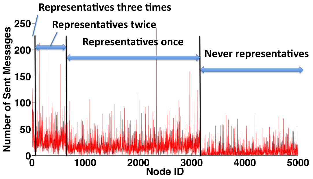
Figure 7 illustrates the typical fraction of transmissions per node as a function of location in the unit square normalized as a probability distribution. Each pixel is assigned an intensity proportional to the number of messages that nodes located in that region will typically transmit. Thus this figure reveals which nodes suffer from the heaviest traffic. The figure is the result of averaging over realizations of gossip for each of different -node random geometric graphs. As the figure shows, multiscale gossip tends to distribute traffic almost uniformly in all the nodes. The observed color pattern is consistent with the hierarchical nature of the algorithm and although nodes that become representatives send more messages, no node is heavily used. On the other hand, for path averaging we observe that the nodes at the center (red region) send many more messages than nodes around the perimeter. This should be expected since geographic routing (which path averaging relies on) is greedy when trying to deliver messages to remote locations across the network.


VIII Discussion and Future Work
We have presented a new algorithm for distributed averaging exploiting hierarchical computation. Multiscale gossip separates the computation in linear phases and achieves very close to linear complexity overall. The key to achieving nearly-linear scaling lies in the way the recursive network partition is constructed. In particular, we argue that refining the network so that subnetworks at scale contain nodes provides optimal message-scaling laws with minimal number of levels in the hierarchy; although other hierarchical partitioning schemes could be constructed to achieve nearly-linear message complexity, they would require deeper hierarchies and, consequently, additional overhead for management. Our analysis focused on network topologies modeled as random geometric graphs, but it should be clear that the results translate directly to grids (-dimensional lattices) embedded in the unit square.
Another feature of the proposed scheme is that the maximum distance any message has to travel is hops, which is shorter than hops needed by path averaging [13], where each iteration involves averaging along a path of nodes potentially spanning the diameter of the network. Requiring transmissions over shorter distances is advantageous when transmitting over unreliable links that use acknowledgements and retransmission to ensure reliable communication at the link-layer, as is common practice in many existing systems. Intuitively, shorter paths translates directly to fewer retransmissions, and we illustrate this via simulation.
There is a number of interesting future directions that we see. In our present algorithm, gossip at higher levels happens on overlay grids which are known to require a number of messages which scales quadratically in the size of the grid. Since these grids already use multi-hop communication, it may be possible to further increase performance by devising other overlay graphs between representatives with better convergence properties, i.e. expander graphs [28]. Moreover, the subdivision of the unit square into a grid cell is not necessarily natural with respect to the topology of the graph, and one could use other methods for constructing hierarchical partitions which are tuned to the network topology. Our preliminary results with using hierarchical spectral clustering appear promising in simulation. It is, however, not clear how to carry out spectral clustering in a decentralized manner way and in linear number of messages. Another possibility is to combine the multiscale approach with the use of more memory at each node to get faster mixing rates. Notice however that how to use memory to provably accelerate asynchronous gossip is still an open question. Current results only consider synchronous algorithms [17]. Finally, an important advantage of gossip algorithms in general is their robustness. However, the general question of modeling and reacting to node failures has not been formally investigated in the literature. It would be very interesting to introduce failures and see the effect on performance for different gossip algorithms.
Appendix A Complementary derivations for multi-scale gossip error bound
Looking at inequality (12), we have three terms that we need to bound.
- •
: We can bound the numerator if we consider the following; At some level we have for some . We can keep bounding all the way down to level in the exact same fashion since for and so on. If we do this for all terms appearing in the vector , we get a numerator as a norm of elements from the initial -vector. Since we need to divide expression by , the ratio is less than one simply since the denominator has more terms. This means .
- •
: Using definition (5) and the fact that an average such as can be written as the average of averages,
(35) Pulling and the summation over out, adding and subtracting the mean, taking the absolute value and using triangular inequality
(36) (37) Using bound (6)
(38) Using definition (5)
(39) Pulling the summation and the term outside
(40) We repeatedly pull out terms and add and subtract means to reach
(42) (44) The comment from bounding helps us here as well. Each term in the numerator can be bounded by terms from the initial vector and dividing by we get
(45) This is true since each summation cancels out with the corresponding denominator leaving only an term and we have such terms. Now obviously
Acknowledgment
This work is supported by grants from the Fonds québécois de la recherche sur la nature et les technologies, and the Mathematics of Information Technology and Complex Systems (MITACS) Canadian network of centers of excellence.
The authors would like to thank Marius Sucan for providing the multi-scale grid figure used in Section III.
References
- [1] K. Tsianos and M. Rabbat, “Fast decentralized averaging via multi-scale gossip,” in Proc. Intl. Conf. on Distributed Computing in Sensor Systems, Santa Barbara, CA, June 2010.
- [2] S. Boyd, A. Ghosh, B. Prabhakar, and D. Shah, “Randomized gossip algorithms,” IEEE Trans. Inf. Theory, vol. 52, no. 6, pp. 2508–2530, Jun. 2006.
- [3] D. Kempe, A. Dobra, and J. Gehrke, “Gossip-based computation of aggregate information,” in Proc. IEEE Foundations of Computer Science, Cambridge, MA, Oct. 2003.
- [4] J. Tsitsiklis, D. Bertsekas, and M. Athans, “Distributed asynchronous deterministic and stochastic gradient optimization algorithms,” IEEE Trans. Automatic Control, vol. AC-31, no. 9, pp. 803–812, Sep. 1986.
- [5] J. Tsitsiklis, “Problems in decentralized decision making and computation,” Ph.D. dissertation, Massachusetts Institute of Tech., Nov. 1984.
- [6] A. Dimakis, S. Kar, J. Moura, M. Rabbat, and A. Scaglione, “Gossip algorithms for distributed signal processing,” 2010, to appear in Proceedings of the IEEE.
- [7] P. Gupta and P. R. Kumar, “Critical power for asymptotic connectivity in wireless networks,” in Stochastic Analysis, Control, Optimization, and Applications, Boston, 1998, pp. 1106–1110.
- [8] S. Mallat, A Wavelet Tour of Signal Processing. Academic Press, 1999.
- [9] A. Özgür, O. Lévêque, and D. Tse, “Hierarchical cooperation achieves optimal capacity scaling in ad hoc networks,” IEEE Trans. Inform. Theory, vol. 53, no. 10, pp. 3549–3572, Oct. 2007.
- [10] M. Nagy, Z. Akos, D. Biro, and T. Vicsek, “Hierarchical group dynamics in pigeon flocks,” Nature, vol. 464, no. 7290, pp. 890–893, Apr. 2010.
- [11] A. Dimakis, A. Sarwate, and M. Wainwright, “Geographic gossip: Efficient averaging for sensor networks,” IEEE Trans. Signal Processing, vol. 56, no. 3, pp. 1205–1216, Mar. 2008.
- [12] R. Sarkar, X. Yin, J. Gao, F. Luo, and X. D. Gu, “Greedy routing with guaranteed delivery using ricci flows,” in Proc. Information Processing in Sensor Networks, San Francisco, April 2009.
- [13] F. Benezit, A. Dimakis, P. Thiran, and M. Vetterli, “Gossip along the way: Order-optimal consensus through randomized path averaging,” in Proc. Allerton Conf. on Comm., Control, and Comp., Urbana-Champaign, IL, Sep. 2007.
- [14] M. Penrose, Random Geometric Graphs. Oxford University Press, 2003.
- [15] M. Cao, D. A. Spielman, and E. M. Yeh, “Accelerated gossip algorithms for distributed computation,” in Proc. 44th Annual Allerton Conf. Comm., Control, and Comp., Monticello, IL, Sep. 2006.
- [16] E. Kokiopoulou and P. Frossard, “Polynomial filtering for fast convergence in distributed consensus,” IEEE Trans. Signal Processing, vol. 57, no. 1, pp. 342–354, Jan. 2009.
- [17] B. Oreshkin, M. Coates, and M. Rabbat, “Optimization and analysis of distributed averaging with short node memory,” To appear IEEE Trans. Signal Processing, 2010.
- [18] W. Li and H. Dai, “Location-aided fast distributed consensus,” in IEEE Transactions on Information Theory, submitted, 2008.
- [19] K. Jung, D. Shah, and J. Shin, “Fast gossip through lifted Markov chains,” in Proc. Allerton Conf. on Comm., Control, and Comp., Urbana-Champaign, IL, Sep. 2007.
- [20] ——, “Distributed averaging via lifted Markov chains,” Aug. 2009, to appear in IEEE Trans. on Info. Theory, and available online as arxiv:0908:4073v1.
- [21] R. Sarkar, X. Zhu, and J. Gao, “Hierarchical spatial gossip for multi-resolution representations in sensor networks,” in Proc. of the International Conference on Information Processing in Sensor Networks (IPSN’07), April 2007, pp. 420–429.
- [22] J.-H. Kim, M. West, S. Lall, E. Scholte, and A. Banaszuk, “Stochastic multiscale approaches to consensus problems,” in Proc. IEEE Conf. on Decision and Control, Cancun, Dec. 2008.
- [23] M. Epstein, K. Lynch, K. Johansson, and R. Murray, “Using hierarchical decomposition to speed up average consensus,” in Proc. IFAC World Congress, Seoul, Jul. 2008.
- [24] F. Cattivelli and A. Sayed, “Hierarchical diffusion algorithms for distributed estimation,” in Proc. IEEE Workshop on Statistical Signal Processing, Wales, Aug. 2009.
- [25] H. T.-H. Chan, A. Gupta, B. M. Maggs, and S. Zhou, “On hierarchical routing in doubling metrics,” Proceedings of the sixteenth annual ACM-SIAM symposium on Discrete algorithms (SODA), pp. 762–771, 2005.
- [26] D. Tschopp, S. Diggavi, and M. Grossglauser, “Hierarchical routing over dynamic wireless networks,” International conference on Measurement and modeling of computer systems (SIGMETRICS), pp. 73–84, 2008.
- [27] C. Avin and G. Ercal, “On the cover time and mixing time of random geometric graphs,” Theoretical Computer Science, vol. 380, pp. 2–22, June 2007.
- [28] G. Margulis, “Explicit group-theoretical constructions of combinatorial schemes and their application to the design of expanders and concentrators,” J. Probl. Inf. Transm., vol. 24, no. 1, pp. 39–46, 1988.