On the conjugacy problem for finite-state automorphisms of
regular rooted trees
with an appendix by Raphaël M. Jungers
Abstract
We study the conjugacy problem in the automorphism group of a regular rooted tree and in its subgroup
of finite-state automorphisms. We show that under the contracting condition and the finiteness of what we call
the orbit-signalizer, two finite-state automorphisms are conjugate in if and only if they are conjugate in
, and that this problem is decidable. We prove that both these conditions are satisfied by bounded automorphisms
and establish that the (simultaneous) conjugacy problem in the group of bounded automata
is decidable.
Mathematics Subject Classification 2010: 20E08, 20F10
Keywords: automorphism of a rooted tree, conjugacy problem, finite-state automorphism, finite automaton, bounded automaton
1 Introduction
The interconnection between automata theory and algebra produced in the last three decades many important constructions such as self-similar groups and semigroups, branch groups, iterated monodromy groups, self-similar (self-iterating) Lie algebras, branch algebras, permutational bimodules, etc. (see [17, 24, 9, 3, 1, 18] and the references therein).
The connection between groups and automata occurs via a natural correspondence between invertible input-output automata over the alphabet and automorphisms of a regular one-rooted -ary tree . To present this correspondence let us index the vertices of the tree by the elements of the free monoid , freely generated by the set and ordered by provided is a prefix of . The group of all automorphisms of the tree decomposes as the permutational wreath product , where is the symmetric group on the set . This decomposition allows us to represent automorphisms in the form , where is the permutation induced by the action of on the first level of the tree . Iteratively, we can define the automorphism for every vertex of the tree , where . Then every automorphism corresponds to an input-output automaton over the alphabet and with the set of states . The automaton transforms the letters as follows: if the automaton is in state and reads a letter then it outputs the letter and the state changes to ; these operations can be best described by the labeled edge . Following the terminology of the automata theory every automorphism is called the state of at .
Using this correspondence with automata one can define several classes of special subgroups of the group . A subgroup is called state-closed or self-similar if all states of every element of are again elements of . Self-similar groups play an important role in modern geometric group theory, and have applications to diverse areas of mathematics. In particular, self-similar groups are connected with fractal geometry through limit spaces and also with dynamical systems through iterated monodromy groups as developed by V. Nekrashevych [17]. The set theoretical union of all finitely generated self-similar subgroups in is a countable group denoted by called the group of functionally recursive automorphisms [5].
Automorphisms of the tree which correspond to finite-state automata are called finite-state. More precisely, an automorphism is finite-state if the set of its states is finite. The set of all finite-states automorphisms forms a countable group denoted by . Every finite-state automorphism is functionally recursive, and hence the group is a subgroup of .
Other natural subgroups of are the groups of polynomial automata of degree for every and their union . These groups were introduced by S. Sidki in [22], who tried to classify subgroups of by the cyclic structure of the associated automata and by the growth of the number of paths in the automata avoiding the trivial state. Especially important is the group of bounded automata whose elements are called bounded automorphisms. A finite-state automorphism is bounded if the number of paths of length in the automaton avoiding the trivial state is bounded independently of . It is to be noted that most of the studied self-similar groups are subgroups of . In particular, the Grigorchuk group [8], the Gupta-Sidki group [12], the Basilica [11] and BSV groups [6], the finite-state spinal groups [3], the iterated monodromy groups of post-critically finite polynomials [17], and many others, are generated by bounded automorphisms. Moreover, it is shown in [4] that finitely generated self-similar subgroups of are precisely those finitely generated self-similar groups whose limit space is a post-critically finite self-similar set which play an important role in the development of analysis on fractals (see [13]).
In this paper we consider the conjugacy problem and the order problem in the groups , , , . It is well known that the word problem is solvable in the group and hence in all its subgroups, while it is an open problem in the group . Furthermore, the order and conjugacy problems are open in and . The conjugacy classes of the group were described in [23, 7]. It is not difficult to construct two finite-state automorphisms which are conjugate in but not conjugate in (see [9]). At the same time, two finite-state automorphisms of finite order are conjugate in if and only if they are conjugate in (see [21]). The conjugacy classes of the group of finitary automorphisms were determined for the binary tree in [5] and for the general case in [19].
The conjugacy problem was solved for some well-known finitely generated subgroups of . In particular, the solution of the conjugacy problem in the Grigorchuk group was given in [14, 20], and it was generalized in [26, 10] to certain classes of branch groups and their subgroups of finite index. Moreover, it was shown in [15] that the conjugacy problem in the Grigorchuk group is decidable in polynomial time. The conjugacy problem for the Basilica and BSV groups was treated in [11]. A finitely generated self-similar subgroup of with unsolvable conjugacy problem was constructed in a recent preprint [25].
The general approach in considering any algorithmic problem dealing with automorphisms of the tree is to reduce the problem to some property of their states. The order and the conjugacy problems lead us to the following definition. For an automorphism consider the orbits of its action on the vertices of the tree and define the set
which we call the orbit-signalizer of . It is not difficult to see that the order problem is decidable for finite-state automorphisms with finite orbit-signalizers. We prove that every bounded automorphism has finite orbit-signalizer and hence the order problem is decidable for bounded automorphisms.
Proposition 1.
The order problem for bounded automorphisms is decidable.
We treat the conjugacy problem firstly in the group . Given two automorphisms we construct a conjugator graph based on the sets , which portrays the inter-dependence among the different conjugacy subproblems encountered in trying to find a conjugator for the pair , and which leads to the construction of a conjugator if it exists.
Theorem 2.
Two finite-state automorphisms with finite orbit-signalizers are conjugate in if and only if they are conjugate in if and only if the conjugator graph is nonempty.
An important class of self-similar groups are contracting groups. This property for groups corresponds to the expanding property in a dynamical system. A finitely generated self-similar group is contracting if the length of its elements asymptotically contracts when applied to their states. A finite-state automorphism is called contracting if the self-similar group generated by its states is contracting. Bounded automorphisms are contracting (see [4]), however in contrast to bounded automorphisms, contracting automorphisms do not form a group. For contracting automorphisms with finite orbit-signalizers, we prove that conjugation is controlled by the group of finite-state automorphisms.
Theorem 3.
Two contracting automorphisms with finite orbit-signalizers are conjugate in if and only if they are conjugate in .
We prove a number of results for the conjugacy problem for bounded automorphisms in Section 4, which we collect in the following theorem.
Theorem 4.
- 1.
The (simultaneous) conjugacy problem for bounded automorphisms in is decidable.
- 2.
Two bounded automorphisms are conjugate in the group if and only if they are conjugate in the group .
- 3.
The (simultaneous) conjugacy problem in is decidable.
- 4.
Two bounded automorphisms are conjugate in the group if and only if they are conjugate in the group .
We develop two algorithms for the solution of the conjugacy problem in the group . The first one exploits the cyclic structure of bounded automorphisms. While the second exploits the number of active states of bounded automorphisms. This last counting argument translates to a bounded trajectory problem for nonnegative matrices which is shown to be decidable in the appendix by Raphaël M. Jurgens. The methods developed in this study provide a construction for possible conjugators whenever the associated conjugacy problems are solved.
The last section presents some examples, which illustrate the solution of the conjugacy problems, and describes the connection between the property of having finite orbit-signalizers and other properties of automorphisms.
2 Preliminaries
The set is considered as the set of vertices of the tree as described in Introduction. The length of a word for is denoted by . The set of words of length forms the -th level of the tree . The vertices are ordered by the lexicographic order on words induced by the order on the set .
We are using right actions, so the image of a vertex under the action of an automorphism is written as or , and hence .
The state of at , which was defined in Introduction, is the unique automorphism of the tree such that the equality holds for all words . Computation of states of automorphisms is done as follows:
for all and . Therefore, conjugation is computed by the rules
and if then
The multiplication of two automorphisms expressed as , is performed by the rule
Every permutation can be identified with the automorphism of the tree acting on the vertices by the rule for and .
The group of functionally recursive automorphisms consists of automorphisms which can be constructed as follows. A finite set of automorphisms is called functionally recursive if there exist words over and permutations such that
This system has a unique solution in the group , here the action of each element on the first level of the tree is given by the permutation , and the action of the state is uniquely defined by the word . An automorphism of the tree is called functionally recursive provided it is an element of some functionally recursive set of automorphisms.
For an automorphism define the numerical sequence
which describes the activity growth of . Looking at the asymptotic behavior of the sequence we can define different classes of automorphisms of the tree .
The elements , whose sequence is eventually zero, are called finitary automorphisms. In other words, an automorphism is finitary if there exists such that for all , and the smallest with this property is called the depth of . The set of all finitary automorphisms forms a group denoted by .
For a finite-state automorphism the sequence can grow either exponentially or polynomially (see [22, Corollary 7]). The set of all finite-state automorphisms , whose sequence is bounded by a polynomial of degree , is the group of polynomial automata of degree . In the case , when the sequence is bounded, then the automorphism is called bounded and the group is called the group of bounded automata. We get an ascending chain of subgroups for . The union is called the group of polynomial automata. If we replace the condition “ acts non-trivially on ” by “ is non-trivial” in the definition of the sequence then we still get the same groups .
The bounded and polynomial automorphisms can be characterized by the cyclic structure of their automata as described in [22]. A cycle in an automaton is called trivial if it is a loop at the state corresponding to the trivial automorphism. Then an automorphism is polynomial if and only if any two different non-trivial cycles in the automaton are disjoint. Moreover, , when is the largest number of non-trivial cycles connected by a directed path. In particular, an automorphism is bounded if and only if any two different non-trivial cycles in the automaton are disjoint and not connected by a directed path. We say that is circuit if there exists a non-empty word such that , i.e. lies on a cycle in the automaton . If is a circuit bounded automorphism then the state is finitary for every word , which is not read along the circuit.
3 Conjugation in groups of automorphisms of the tree
Let us recall the description of the conjugacy classes in the group .
Conjugacy classes in . First, recall that every conjugacy class of the symmetric group has a unique (left-oriented) representative of the form
| (1) |
where and . This observation can be generalized to the group (see [23, Section 4.1]). Given an automorphism in we can conjugate it to a unique (left-oriented) representative of its conjugacy class using the following basic steps.
1. Conjugate the permutation to its unique left-oriented conjugacy representative (1).
2. Consider every cycle in the representative (1) of and define
Conjugate by the the automorphism to obtain , where
3. Apply the steps 1 and 2 to the automorphisms .
It is direct to see that an infinite iteration of this procedure produces a well-defined automorphism of the tree which conjugates into a representative and that two different representatives are not conjugate in .
Another approach is based on the fact that two permutations are conjugate if and only if they have the same cycle type. The orbit type of an automorphism is the labeled graph, whose vertices are the orbits of on , every orbit is labeled by its cardinality, and we connect two orbits and by an edge if there exist vertices and , which are adjacent in the tree . Then two automorphisms of the tree are conjugate if and only if their orbit types are isomorphic as labeled graphs (see [7, Theorem 3.1]). In particular it follows, that the group is ambivalent (that is, every element is conjugate with its inverse). More generally, every automorphism is conjugate with for every unit of the ring of -adic integers, where is the exponent of the group (see [23, Section 4.3]).
Conjugation lemma. We say that an element is a conjugator for the pair if , and we use the notation . For and the permutations induced by the action of and on , the set of permutational conjugators for the pair is denoted by
(this set can be empty).
The study of the conjugacy problem in the automorphism groups of the tree is based on the following standard lemma.
Lemma 1.
Let .
- 1.
If then for every and
where .
- 2.
Let be the orbits of the action of on . If there exists such that and are conjugate in for every , where is an arbitrary point, then and are conjugate in .
Proof.
The first statement follows from the equalities , .
Let , where . Put , then , where and . Then
Multiplying these equations, we get
In particular
| (2) |
∎
If and are finite-state automorphisms (we need this only for the word problem), Lemma 1 suggests a branching decision procedure for the conjugacy problem in . We call this procedure by CP and remark that it may not stop in general.
The order problem in . The problem of finding the order of a given element of can be handled in a manner similar to the above. The next observation gives a simple condition used in many papers to prove that an automorphism has infinite order.
Lemma 2.
Let .
- 1.
Let be the orbits of the action of on . Define for every , where and is an arbitrary point. The automorphism has finite order if and only if all the states have finite order. Moreover, in this case, the order of is equal to
- 2.
Suppose for some choice of . If then has infinite order. If then has finite order if and only if has finite order for all , in which case we can remove the term from the right hand side of the above equality.
If is a finite-state automorphism, then the word problem can be effectively solved and Lemma 2 suggests a branching procedure to find the order of a. We call this procedure by OP and remark that it may not stop in general. Such a procedure is implemented in the program packages [2, 16].
Orbit-signalizer. Lemmas 1 and 2 lead us to define the orbit-signalizer of an automorphism as the set
which contains all automorphisms that may appear in the procedures OP and CP. Notice that if , , and then and
| (3) |
This observation implies the recursive procedure to find the set . We start from the set and compute consecutively
Then . It follows from construction that if does not contain new elements, i.e., , then we can stop and . In particular, if the set is finite, then this procedure stops in finite time and we can find algorithmically. For automorphisms with finite orbit-signalizers one can model the procedures OP and CP by finite graphs.
Order graph. Consider an automorphism which has finite orbit-signalizer. We construct a finite graph with the set of vertices , called the order graph of , which models the branching procedure OP. The edges of this graph are constructed as follows. For every consider all orbits of the action of on and let be the least element in . It is easy to see that for , and we introduce the labeled edge in the graph for every . Then Lemma 2 can be reformulated as follows.
Proposition 5.
Let have finite orbit-signalizer. Then has finite order if and only if all edges in the directed cycles in the order graph are labeled by .
Moreover, in this case we can compute the order of using the graph . Remove all the edges of every directed cycle in . Then the only dead vertex of , i.e. the vertex without outgoing edges, is the trivial automorphism, which has order . Then inductively, for consider all outgoing edges from , and let be the edge labels and be the corresponding end vertices, whose order we already know. Then by Lemma 2 the order of is equal to the least common multiple of . We illustrate the construction of the order graph and the solution of the order problem in Example 2 of Section 5.
Conjugator graph. Consider automorphisms both of which have finite orbit-signalizers. We construct a finite graph , called the conjugator graph of the pair , modeled after the branching procedure CP of Lemma 1. The vertices of the graph are the triples for , , and whenever this last set is nonempty. The edges are constructed as follows.
Let for be the orbits of in its action on and let denote the least element in each . We will simplify the notation by writing instead and with the understanding that these refer to under consideration.
For any vertex , if one of the sets with is empty, then the triple is a dead vertex. Otherwise we introduce in the graph the edge
for every and . Notice that , , and hence the triple is indeed a vertex of the graph.
We simplify the graph obtained above using the following reductions. Remove the vertex which does not have an outgoing edge labeled by for some . Also, remove all edges leading to these deleted vertices. We repeat the reductions as long as possible to reach the graph .
If the graph is empty, then the automorphisms and are not conjugate. Otherwise they are conjugate and every conjugator can be constructed level by level as follows. Choose any vertex in and define the action of on the first level by for . There is an outgoing edge from labeled by , as explained previously. Choose an edge for every and let be the corresponding end vertex. We define the action of the state by the rule for . All the other states of on the vertices of the first level are uniquely defined by Equation (2) at the end of the proof of Lemma 1, and thus we get the action of on the second level. Similarly, we proceed further with the vertices and construct the action of on the third level, and so on. Notice that even if the same vertex appears at different stages of the definition of we still have a freedom to choose different outgoing edges from in each stage of the construction.
Basic conjugators. Let us construct certain conjugators, called basic conjugators for the pair , by making as few choices as possible, in the sense that if we arrive at a triple at some stage of the construction then we choose the same permutation whenever the pair reappears further down. That is, for every two vertices and obtained under construction we insist to have . More precisely every basic conjugator can be defined using special subgraphs of the conjugator graph . Consider the subgraph of , which satisfies the following properties:
- 1.
The subgraph contains some vertex for .
- 2.
For every vertex of and every letter , there exists precisely one outgoing edge from labeled by . In particular, the graph is deterministic, and the number of outgoing edges at the vertex of the graph is equal to the number of orbits of on .
- 3.
For every and there is at most one vertex of the form in the graph . In other words, if and are vertices of then .
If the graph is nonempty, there always exist subgraphs of , which satisfy the properties 1-3. For every such a subgraph we construct the basic conjugator as follows. We construct a functionally recursive system involving every conjugator , where is a vertex of and thus in particular, we construct . First, we define the action of the conjugator on the first level by the rule for , where the permutation is uniquely defined such that the triple is a vertex of . For every edge we define the states of the conjugator on the letters from the orbit of under recursively by the rule
for . These rules completely define the automorphisms . By Lemma 1 every constructed automorphism is indeed a conjugator for the pair . Since the graph is finite, and the automorphisms are finite-state, we get a functionally recursive system which uniquely defines the basic conjugator given by the subgraph .
We have proved the following theorem.
Theorem 6.
Let have finite orbit-signalizers, and let be the corresponding conjugator graph. Then and are conjugate in if and only if they are conjugate in if and only if the graph is nonempty.
In particular, the conjugacy problem for finite-state automorphisms with finite orbit-signalizers is decidable in the groups and . We present examples of the construction of the conjugator graph and basic conjugators in Example 3 of Section 5.
The same method works for the simultaneous conjugacy problem, which given automorphisms and asks for the existence of an automorphism such that for all . We again consider the permutations such that for all , take an orbit of on , let be the least element and . Then the problem reduces to the simultaneous conjugacy problem for and . If automorphisms and are finite-state and have finite orbit-signalizers, then we can similarly construct the associated conjugator graph so that Theorem 6 holds.
Conjugation of contracting automorphisms. A self-similar subgroup is called contracting if there exists a finite set with the property that for every there exists such that for all words of length . The smallest set with this property is called the nucleus of the group. An automorphisms is called contracting if the self-similar group generated by all states of is contracting. It follows from the definition that contracting automorphisms are finite-state.
Theorem 7.
Two contracting automorphisms with finite orbit-signalizers are conjugate in the group if and only if they are conjugate in the group .
Proof.
We will prove that all the basic conjugators for the pair are finite-state. We need a few lemmata, which are interesting in themselves.
Lemma 3.
Let be a contracting self-similar group, and let be a finite subset of . Then the set of all possible elements of the form
where and , is finite.
Proof.
The statement is a reformulation of Proposition 2.11.5 in [17]. We sketch the proof for completeness.
We can assume that the set is self-similar, i.e. for all and (all the elements are finite-state), and contains the nucleus of the group . There exists a number such that for all words of length . Then for all and . It is sufficient to prove that there are finitely many elements of the form
for and . Then and . Inductively we get that all the above elements belong to . ∎
The next lemma is similar to Corollary 2.11.7 in [17], which states that different self-similar contracting actions with the same virtual endomorphism are conjugate via a finite-state automorphism.
Lemma 4.
Let be a contracting self-similar group and be a finite subset. Suppose that the automorphism satisfies the condition that for every there exist such that . Then is finite-state.
Proof.
For an arbitrary word we have
| (4) |
where are some elements in , and . By Lemma 3 the above products assume a finite number of values, and hence is finite-state. ∎
Notice that in the previous lemma we only need that the groups generated by all states of and separately by all states of be contracting, while together they may generate a non-contracting group.
Lemma 5.
Let be a finite collection of automorphisms. Suppose that there exist two contracting self-similar groups , and finite subsets , with the condition that for every and every letter there exist , and such that . Then all the automorphisms in are finite-state.
Proof.
Example 4 of Section 5 shows that we cannot drop the assumption about orbit-signalizers in the theorem.
The finiteness of orbit-signalizers can be used to prove that certain automorphisms are not conjugate in the group .
Proposition 8.
Let be conjugate in . Then has finite orbit-signalizer if and only if does.
Proof.
Let for a finite-state automorphism , and suppose has finite orbit-signalizer. Then for every and
It follows that , where is the set of states of , and hence the set is finite. ∎
4 Conjugation of bounded automorphisms
How to check that a given finite-state automorphism has finite orbit-signalizer is yet another algorithmic problem. Let us show that some classes of automorphisms have finite orbit-signalizers. Every finite-state automorphism of finite order has finite orbit-signalizer. Here the set is bounded by the number of all states of all powers of , which is finite. In particular, if a finite-state automorphism has infinite orbit-signalizer, then it has infinite order.
Proposition 9.
Every bounded automorphism has finite orbit-signalizer.
Proof.
Let be a bounded automorphism, and choose a constant so that the number of non-trivial states for is not greater than for every . Then for every vertex the state with is a product of no more than states of , which is a finite set. ∎
In particular, the orbit-signalizer of a bounded automorphism can be computed algorithmically, the procedure CP solves the conjugacy problem for bounded automorphism in , and the procedure OP finds the order of a bounded automorphism.
Corollary 10.
(1). The order problem for bounded automorphisms is decidable.
(2). The (simultaneous) conjugacy problem for
bounded automorphisms in is decidable.
Theorem 11.
Two bounded automorphisms are conjugate in the group if and only if they are conjugate in the group .
Proof.
Corollary 12.
Let be a bounded automorphism. Then and are conjugate in .
Corollary 13.
Let a bounded automorphism and a contracting automorphism be conjugate in . Then and are conjugate in if and only if has finite orbit-signalizer.
4.1 Decision of conjugation between bounded automorphisms by a finitary automorphism
Consider the conjugacy problem for bounded automorphisms in the group of finitary automorphisms. One of the approaches is to restrict the depth of a possible finitary conjugator. Let be two bounded automorphisms. If and are conjugate in and is a finitary conjugator then every state for is a finitary conjugator for the pair with , and has less depth than . However, it is possible that every pair for with is conjugate via a finitary conjugator of depth , while is not conjugate via a finitary conjugator of depth . Hence we still do not get a bound on the depth of even if we know the bound on the depth of a finitary conjugator for every pair . The problem is that we need to find a finitary conjugator for the pair so that all elements for are finitary. To overcome this difficulty we introduce configurations of orbits, which describe these dependencies.
Configurations of orbits. Every configuration will be of the form , where is a pair of automorphism called the main pair of , and is the set of pairs of automorphism called dependent pairs. Configurations for the pair are constructed recursively as follows. At zero level we have just one configuration , where . Further we construct recursively the set from the set . Take a configuration , . Consider every orbit of the action of on , let be the least element in and . For every define new configuration , where
| (5) |
The set consists of all configurations constructed in this way. Then is the set of configurations for . It follows from construction that if does not contain new configurations, i.e., , then we can stop and . In particular, if the set is finite then it can be computed algorithmically.
Lemma 6.
The set of configurations for a pair of bounded automorphisms is finite and can be computed algorithmically.
Proof.
Let be a configuration for and denote . We prove by induction that there exists a word such that
| (6) |
where . The basis of induction is the initial configuration that satisfies this condition for the empty word . Suppose inductively that a configuration satisfies the condition for a word and proceed with the construction of . Let be the least element in an orbit of the action of on and put . Then and we get
Hence satisfies condition (6) for the word .
In particular, and can assume only a finite number of values. The number of different sets , , for a bounded automorphism , is finite (the proof is the same as of Proposition 9). Hence there are finitely many possibilities for the set . The same observation holds for and the set . It follows that the number of configurations for a pair of bounded automorphisms is finite. ∎
Remark 1.
Let . Let be an orbit of the action of on and be the least element in the orbit and . Then , where
is a configuration for .
Configurations satisfied by a finitary automorphism. We say that a finitary automorphism satisfies a configuration if is a conjugator for the main pair of and all elements for are finitary. We say that a configuration has depth if is satisfied by a finitary automorphism of depth and all elements for have depth . In particular, the automorphisms are conjugate in if and only if the configuration is satisfied by a finitary automorphism. Let us show that it is decidable whether a given configuration can be satisfied by a finitary automorphism.
Lemma 7.
Let be a configuration. Consider all orbits of the action of on and let be the least element in . The configuration has depth if and only if there exists such that every configuration , , has depth .
Proof.
Suppose and all automorphisms , , are finitary of depth . For the permutation in we take . Then
and for every and we get
| (7) |
where . All automorphisms are finitary of depth . Hence every configuration has depth .
Conversely, suppose there exists such that every is satisfied by a finitary automorphism . Define automorphism by the rules and
Note that for and hence every pair belongs to . Therefore the automorphism is finitary. Also is a conjugator for by construction and satisfies the configuration by Equation (7). ∎
Corollary 14.
If and are conjugate in then there exists a finitary conjugator of depth . In particular, the conjugacy problem for bounded automorphisms in the group is decidable.
Instead of just running through all finitary automorphisms with a given bound on the depth, the algorithm can be realized as follows. Construct the set of all configuration for a given pair . We will consecutively label configurations by numbers which correspond to their depths. First, we identify configurations of depth , which are precisely configurations such that and for all . Then iteratively we label a configuration by number if there exists such that each is already labeled by a number . After this process finishes, the configurations labeled by can be satisfied by a finitary automorphisms of depth , while the unlabeled configurations cannot be satisfied by finitary automorphisms.
4.2 The conjugacy problem in the group of bounded automata
In this subsection we prove that the conjugacy problem in the group of bounded automata is decidable. We will show two approaches.
First approach: by using cyclic structure of bounded automata. Let and be bounded automorphisms. We apply the following algorithm to check whether and are conjugate in . The algorithm will consecutively determine the pairs from that are conjugate in . Further we prove that the algorithm is correct.
Step 1. Take and compute the set of all configurations for . For every configuration and every check whether and are conjugate in , and if yes then are conjugate in . Apply this step to every pair . Note that since is a configuration for we also detect every pair conjugated in (just take ).
Step 2. Take . Consider all words such that and . Consider all circuit automorphisms such that and every finitary state of has depth . Note that there are only finitely many bounded automorphisms with these properties. For every such check whether . We apply this step to every pair not detected in Step .
Step 3. For every pair for which we still do not know whether it is conjugate in proceed as follows. Consider orbits of the action of on , let be the least element in the orbit and . Check whether there exists such that for every pair (it belongs to ) we already know that it is conjugate in . If yes then are conjugate in . We repeat this step as long as possible until no new pairs are detected. The other pairs from are not conjugate in .
Proof of correctness of the algorithm.
First, every pair detected in one of the steps is indeed conjugate in . We need to prove the converse that if are conjugate in then the pair will be detected. Let for a bounded automorphism . There exists a level such that for every the state is either circuit or finitary. Consider the orbits of the action of on . Let be the least element in an orbit and . Then is a conjugator for the pair .
If is finitary then the pair is detected in Step .
If is circuit then we take a circuit conjugator for having a circuit of the shortest length. Let be the word which is read along the circuit, so here . Now consider two cases.
Case 1: . Then is finitary. Since we get and
Hence and are conjugate in . Let be the least element in the orbit and . Let be the configuration for associated to the orbit and the conjugator (see Remark 1). Put , , , and note that . Then and . Therefore the pair is detected in Step .
Case 2: . In this case the states of along the circuit do not have dependencies, and we have a freedom to change these states without changing other states of the same level. Suppose there are two states and along the circuit (let so is a prefix of ), which solve the same conjugacy problem . Define the automorphism by the rules , for , and the action of on is the same as the action of . Then is a circuit bounded conjugator for the pair and it has smaller circuit length; we arrive at contradiction. Hence, the states of along the circuit solve different conjugacy problems and therefore . Now consider finitary states of . We can assume that is chosen is such a way that the value of , where ranges over all finitary states of , is the smallest possible over all conjugators for with . Let be a finitary state. Then every state of along the orbit of under is finitary. Hence the configuration for that corresponds to the orbit of is satisfied by a finitary automorphism. However the depth of is not greater than by Lemma 7. Hence the depth of every state of along the orbit of is not greater than . Therefore satisfies the conditions in Step 2 and the pair is detected in this step.
We have proved that every pair from the action of on is detected in Steps . The other pairs coming from the orbits of the action of on smaller levels, in particular the pair , are detected in Step . ∎
Second approach: by calculation of active states. Let be two bounded automorphisms. We check whether are conjugate in and if not then they are not conjugate in . So further we assume that are conjugate in . Every conjugator for the pair can be constructed level by level as described in Section 3 on page 10, by choosing the conjugating permutation for every orbit of . The number of orbits may grow when we pass from one level to the next, and consequently the number of choices grows. However the number of configurations of orbits is finite, and it is easy to see (and also follows from the previous method) that if and are conjugate in then there exists a bounded conjugator such that for all orbits of the same level and of the same configuration the corresponding states of are the same. Hence it is sufficient to choose a conjugating permutation only for configurations. We will show how to count the number of active states depending on our choice.
Suppose we have constructed a conjugator up to the -th level. Consider an orbit of the action of on and let be its configuration (see Remark 1) and be the least element in . The set remembers only the pairs which appear in the formula , here and for ; we will call a state of type . However the number of states of type is lost in this way. To preserve this information we introduce the nonnegative integer column-vector of dimension , where for is equal to the number of such that and . When we pass to the next level, we choose some permutation and define for . Then we check which states of on the vertices from the orbit are active and which are not: the state of type is active if the permutation is non-trivial. We store this information in the row-vector of dimension by making if and otherwise. Hence, when we choose the permutation then the number of active states of along the orbit is equal to .
Let be the set of all configurations for the pair . Let , where and is the main pair of . We view as the set of choices, so that when we choose we have chosen a conjugating permutation for every configuration. The sets and are finite. For define and construct the square nonnegative integer matrix of dimension , where the rows and columns of are indexed by pairs with . The entry of in the intersection of -row and -column is calculated as follows. Recall the construction of configurations induced by and , and given in Equation (5). Let be the main pair of , consider orbits of the action of on , let be the least element in and . Let be the induced configurations. Define the -entry of as
In other words, the -entry of is equal to the number of pairs of type and of configuration induced by one pair from configuration . Now if we have a column-vector , where is the number of states of type and of configuration that we have at certain level, and we choose , then the number of pairs of each configuration on the next level is given by the vector . Put .
Now consider all orbits of on , take their configurations with respect to defined up to the -th level, and define the column-vector as above. To define the action of on the -st level we choose , and for every orbit with configuration we define the action of the states of along this orbit using permutation as usual (we choose a permutation for every configuration even if not all configurations appear on the -th level). In this way the conjugator is defined up to the -st level. Then the number of active states of on the -th level is equal to . The vector , where is equal to the number of all states of type over all orbits of on with configuration , is equal to .
The process starts at the zero level, where we have the vector such that for the configuration , which corresponds to the pair , and for all other pairs and configurations. Then we make choices from and construct the conjugator . It follows from the above discussion that the activity of can be calculated by the following rules:
for all . If there is a choice such that the sequence is bounded, then there will be an eventually periodic choice, and hence the constructed conjugator will be finite-state and bounded.
Hence the automorphisms and are conjugate in the group if and only if there exists a sequence such that the corresponding sequence is bounded. The last problem is solvable and can be deduced from the result presented in Appendix.
In this method we don’t need to solve the auxiliary conjugacy problems in as in the previous method, but the problem reduces to certain matrix problem which should also be solved, while the previous method was direct. We demonstrate both approaches in Examples 5 and 6 of Section 5.
We note that both approaches also solve the respective simultaneous conjugacy problems. We have proved the following theorem.
Theorem 15.
The (simultaneous) conjugacy problem in the group of bounded automata is decidable.
The above methods not only solve the studied conjugacy problem but also provide a construction for a possible conjugator.
Similarly, one can solve the conjugacy problem for bounded automorphisms in every group . However, we have a stronger statement.
Proposition 16.
Two bounded automorphisms are conjugate in the group if and only if they are conjugate in the group .
Proof.
Let and be two bounded automorphisms, which are conjugate in for . We proceed as in the first method above. Again the problem reduces to the case when a conjugator lies on a circuit. Let be the word which is read along the circuit so that . We consider the two cases as in the proof of correctness of the first approach.
If then the state should be in . But then, . Hence, and are conjugate in . The same arguments work if for some word of the form .
Suppose for every word of the form . Then . If (and hence ) then define the automorphism by the rules , for all , , and the action of on is the same as that of . Then belongs to and it is a conjugator for .
If for every word , then some state is a circuit automorphism and for some word of the form . Without loss of generality we can suppose that and . Then the states and are finitary for all , . Consider every orbit of the action of on , let be the least element in and . Then the finitary automorphisms and are conjugate in , and hence they are conjugate in . Define the automorphism by the rules: the action of on is the same as that of , , is a finitary conjugator for the pair , and (also finitary) for every and every orbit . Then is a bounded conjugator for the pair .
Inductively we get that and are conjugate in . ∎
5 Examples
All examples will be over the binary alphabet .
We will frequently use the automorphism given by the recursion , where is a transposition, which is called the (binary) adding machine. The automorphism has infinite order, and acts transitively on each level of the tree . In particular, every automorphism which acts transitively on for all , is conjugate with in the group .
In the next example we investigate the interplay between such properties as being finite-state, contracting, bounded, polynomial, having or not a finite orbit-signalizer.
Example 1.
The adding machine is a bounded automorphism, hence it is contracting and has finite orbit-signalizer, here .
The automorphism given by the recursion is finite-state, , belongs to , and . However is not contracting, because all elements for are different and would belong to the nucleus.
The automorphisms , belong to , but they have infinite orbit-signalizers. All elements for are different and belong to the set . At the same time, and are contracting, for the self-similar group generated by has nucleus .
The automorphism is non-polynomial, contracting, and has finite orbit-signalizer, here .
The automorphism is contracting, the nucleus of the group is . At the same time, the group is not contracting; for and its powers are different and would be in the nucleus.
The automorphism is functionally recursive but not finite-state. Hence the automorphism is functionally recursive, not finite-state, and has finite orbit-signalizer, here .
In the next example we illustrate the solution of the order problem.
Example 2.
Consider the automorphisms and . The order graph is a subgraph of shown in Figure 1. There is a cycle labeled by , hence and have infinite order.
The order graph for the automorphism is shown in Figure 1. There are no cycles with labels , hence has finite order, here .
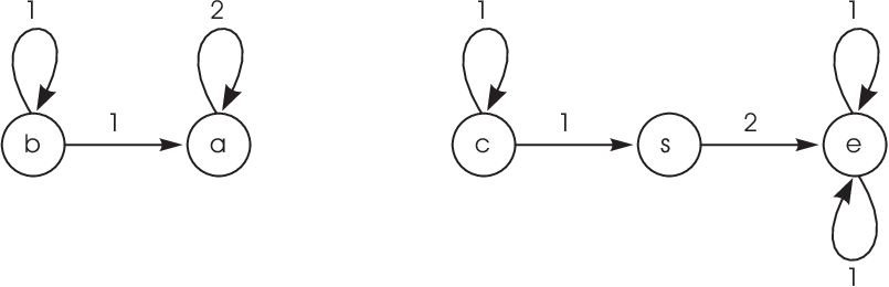
Let us illustrate the construction of the conjugator graph and basic conjugators.
Example 3.
Consider the conjugacy problem for the trivial automorphism with itself. Here and . The conjugator graph is shown in Figure 2. There are two defining subgraphs of the graph , each consists of the one vertex with loops in it for . The corresponding basic conjugators are and .
Consider the conjugacy problem for the adding machine and its inverse . Here , , and . There is one orbit of the action of on , and for every . The conjugator graph is shown in Figure 2. There are two defining subgraphs of the graph , each consists of the one vertex with loop in it for . The corresponding basic conjugators are and .
Consider the conjugacy problem for the adding machine and the automorphism . Here , , and . There is one orbit of the action of on , , , and for every . The conjugator graph is shown in Figure 2. There are four defining subgraphs of the graph , each consists of the two vertices and with the induced edges for . The corresponding basic conjugators are defined as follows
where are actually the basic conjugators for the pair .

The next example shows that the condition of having finite orbit-signalizers cannot be dropped in Theorem 7, and that Theorem 11 does not hold for polynomial automorphisms.
Example 4.
Consider the automorphisms , defined in Example 1. Inductively one can prove that the state is active for every , and hence the automorphism acts transitively on for every . Thus and have the same orbit types (see page 3) and therefore they are conjugate in the group . Both and are contracting, however, has infinite orbit-signalizer, and hence it is not conjugate with in the group , by Proposition 8.
Finally, we illustrate the solution of the conjugacy problem in the group of bounded automata.
Example 5.
Consider the conjugacy problem for the adding machine and its inverse in the group of bounded automata.
There are two configurations for the pair :
Neither of them is satisfied by the trivial automorphism, and hence by a finitary automorphism. In particular, and are not conjugate in the group . The pair is not detected in Step 1 of the first approach, basically, because is not conjugate in . There are no that satisfy Step 2, because has no fixed vertices. Hence, and are not conjugate in the group .
For the second method we get the choice set . The configuration induces the configuration on the next level when we choose the conjugating permutation ; here the pair induces one pair and one pair . For the choice , the configuration induces , and the pair gives two pairs . For the choice , the configuration induces , here the pair induces one pair and one pair , and the pair gives two pairs . For the choice , the configuration induces , here the pair gives two pairs , and the pair gives one pair and one pair . We get the following set of matrices and vectors :
The initial vector is and on -th step we get and when we choose . For any choice the sequence has exponential growth, and hence and are not conjugate in the group of polynomial automata.
Example 6.
Consider the conjugacy problem for the bounded automorphisms and . Notice that the pairs , and , are not conjugate in . Hence, only may appear as the action on of a possible conjugator, and we take . Here and , . The configurations for the pair are the following:
Let us check what configurations are satisfied by a finitary automorphism as described after Corollary 14. The configurations and are satisfied by the trivial automorphism and have depth . For we get that the configuration induced by is equal to . Therefore is not satisfied by a finitary automorphism, and hence and are not conjugate in . In Step 1 of the first approach we detect pairs and . In Step 2 if we take and then . Hence is detected in Step 2 and are conjugate in the group .
For the second method, we take for the choice set . All matrices are the same for . The vectors are as follows
The initial vector is and independently of our choice. If we choose for all then the sequence is bounded. Hence and are conjugate in the group . The conjugator corresponding to our choice is the adding machine .
References
- [1] L. Bartholdi, Branch rings, thinned rings, tree enveloping rings. Israel J. Math. 154 (2006), 93–139.
- [2] L. Bartholdi, FR – GAP package for computations with functionally recursive groups, Version 1.1.2, 2010.
- [3] L. Bartholdi, R.I. Grigorchuk, Z. Sunik, Branch groups. In Handbook of algebra, vol. 3, North-Holland, Amsterdam 2003, 989–1112.
- [4] E.V. Bondarenko and V.V. Nekrashevych, Post-critically finite self-similar groups. Algebra Discrete Math. 4 (2003), 21–32.
- [5] A. Brunner and S. Sidki, On the automorphism group of one-rooted binary trees. J. Algebra 195 (1997), 465–486.
- [6] A. Brunner, S. Sidki, A. Vieira, A just-nonsolvable torsion-free group defined on the binary tree. J. Algebra 211 (1999), 99–114.
- [7] P.W. Gawron, V.V. Nekrashevych, V.I. Sushchansky, Conjugation in tree automorphism groups. Int. J. Algebra Comput. 11 (2001), no. 5, 529–547.
- [8] R.I. Grigorchuk, On the Burnside problem on periodic groups. Functional Anal. Appl. 14 (1980), 41–43.
- [9] R.I. Grigorchuk, V.V. Nekrashevych, V.I. Suschanskii, Automata, dynamical systems, and groups. Proc. Steklov Institute 231 (2000), 128–203.
- [10] R.I. Grigorchuk and J.S. Wilson, The conjugacy problem for certain branch groups. Proc. Steklov Inst. Math. 231 (2000), no. 4, 204–219.
- [11] R.I. Grigorchuk and A. Zuk. Spectral properties of a torsion-free weakly branch group defined by a three state automaton. Contemp. Math. 298 (2002), 57–82.
- [12] N. Gupta and S. Sidki, Some infinite -groups. Algebra i Logica (1983), p.584-598.
- [13] Jun Kigami, Analysis on fractals, Volume 143 of Cambridge Tracts in Mathematics, University Press, Cambridge 2001.
- [14] Y.G. Leonov, The conjugacy problem in a class of -groups. Mat. Zametki 64 (1998), 573–583.
- [15] I. Lysenok, A. Myasnikov, A. Ushakov, The conjugacy problem in the Grigorchuk Group is polynomial time decidable. Groups, Geometry, and Dynamics 4 (2010), 813–833.
- [16] Y. Muntyan and D. Savchuk, AutomGrp – GAP package for computations in self-similar groups and semigroups, Version 1.1.2, 2008.
- [17] V. Nekrashevych, Self-similar groups. Volume 117 of Mathematical Surveys and Monographs, American Mathematical Society, Providence, RI 2005.
- [18] V.M. Petrogradsky, I.P. Shestakov, E. Zelmanov, Nil graded self-similar algebras. Groups, Geometry, and Dynamics 4 (2010), 873–900.
- [19] M.R. Ribeiro, O grupo Finitario de Isometrias da Arvore -ária (The finitary group of isometries of the -ary tree). Doctoral Thesis, Universidade de Brasília 2008.
- [20] A.V. Rozhkov, Conjugacy problem in an automorphism group of an infinite tree. Mat. Zametki 64 (1998), 592–597 .
- [21] A.V. Russev, On conjugacy in groups of finite-state automorphisms of rooted trees. Ukr. Mat. Zh. 60 (2008), no. 10, 1357–1366.
- [22] S. Sidki, Automorphisms of one-rooted trees: growth, circuit structure, and acyclicity. J. Math. Sci. (New York). 100 (2000), no. 1, 1925–1943.
- [23] S. Sidki, Regular trees and their automorphisms. Monografias de Matematica 56, IMPA, Rio de Janeiro 1998.
- [24] S. Sidki, Functionally recursive rings of matrices – two examples. J. of Algebra 322 (2009), 4408–4429.
- [25] Z. Sunic and E. Ventura, The conjugacy problem is not solvable in automaton groups. Preprint, avilable at http://arxiv.org/abs/1010.1993.
- [26] J.S. Wilson and P.A. Zalesskii, Conjugacy seperability of certain torsion groups. Arch. Math. 68 (1997), 441–449.
Appendix A On the existence of a bounded trajectory for nonnegative integer systems
Raphaël M. Jungers
The purpose of this note is to prove the following theorem.
Theorem 17.
The following bounded trajectory problem is decidable.
INSTANCE: A finite set of nonnegative integer matrices and a finite set of nonnegative integer vectors .
PROBLEM: Determine whether there exists a sequence and an initial vector such that the sequence of vectors determined by the recurrence
| (8) |
is bounded.
In the following, denote respectively the set of all products of matrices in and the set of all products of length of matrices in
This problem is closely related to the so called joint spectral subradius of a set of matrices, which is the smallest asymptotic rate of growth of any long product of matrices in the set, when the length of the product increases. For a survey on the joint spectral subradius and similar quantities, see [2]. While the joint spectral subradius is notoriously Turing-uncomputable in general, we will see that in our precise situation, we are able to provide an algorithmic solution to the problem.
The next lemma states that if there is a bounded trajectory, then it can be obtained with an eventually periodic sequence of matrices.
Lemma 8.
Let be an instance of the bounded trajectory problem. There exists a sequence as given by Equation (8) which is bounded if and only if there exist matrices and a vector such that the sequence is bounded.
Proof.
The if-part is obvious. In the other direction, if the set is bounded it must be finite. Thus, there actually exist such that and . ∎
As it turns out it is possible to check in polynomial time, given a nonnegative integer matrix and a vector whether the sequence is bounded. In fact, as we show below, this does not really depend on the actual value of the entries of and but only for each entry of whether it is equal to zero, one, or larger than one, and for each entry of whether it is equal to zero or larger than zero. For this reason we introduce two operators that get rid of the inessential information.
Definition 1.
Given any nonnegative matrix (or vector) , we denote by the matrix in in which all entries larger than two are set to two, while the other entries are equal to the corresponding ones in .
Similarly, we denote by the matrix in in which all entries larger than zero are set to one, while the other entries are equal to zero.
We can now prove the main ingredient of our algorithm.
Theorem 18.
Given a nonnegative matrix , and two indices the sequence remains bounded when grows if and only if the sequence remains bounded. Moreover, the boundedness of the sequence can be checked in polynomial time.
Proof.
We consider the matrix as the adjacency matrix of a directed graph on vertices. The edges of this graph are given by the nonzero entries of . The graph may have loops, i.e., edges from a node to itself, which correspond to diagonal entries. We say that there is a path (of length ) from to if there is a power of such that Equivalently, there exist indices such that for all . It is obvious that if there is a path from to then there is such a path of length less than .
We recall some easy facts from graph theory (see [3] for proofs and references). For any directed graph, there is a partition of the set of its vertices in nonempty disjoint sets (the strongly connected components) such that for all there is a path from to and a path from to if and only if they belong to the same set in the partition. If there is no path from to itself, then is said to be a trivial connected component. Moreover there exists a (non necessarily unique) ordering of the subsets in the partition such that for any two vertices , there cannot be a path from to whenever . There is an algorithm to obtain this partition in operations (with the number of vertices). In matrix terms, this means that one can find a permutation matrix such that the matrix is in block upper diagonal form, where each block on the diagonal corresponds to a strongly connected component.
In the following, we suppose for the sake of clarity that is already in block triangular shape. It is clear that entries in the blocks under the diagonal remain equal to zero in any power of We need a different treatment for the entries within diagonal blocks and the entries in blocks above the diagonal.
- •
Diagonal blocks. Let us consider an arbitrary diagonal block , which is strongly connected by definition. It is easy to see that either all the entries in the block remain bounded or all the entries are unbounded. This occurs if and only if the spectral radius of is larger than one. It is easy to see that given a nonnegative matrix with integer entries whose corresponding graph is strongly connected, its spectral radius is larger than one if and only if one of these conditions is satisfied:
- –
There is an entry in larger than one.
- –
There is a row in with two entries larger than zero.
Observe that these conditions do only depend on
- –
- •
Non-diagonal blocks. Let us consider a particular -entry in a non-diagonal block. We will prove that this entry is unbounded if and only if one of the following conditions holds (and these conditions can be checked in polynomial time):
- I.
There is a path from to and one of the entries is unbounded for
- II.
There exists such that
(9) Moreover, if this condition holds, there is such a smaller than [3, Proposition 1].
- III.
There exist two indices such that there is a path from to , a path from to and such that the pair satisfies condition II above.
- I.
It is straightforward to check that any of these three conditions implies that the -entry is unbounded.
We claim that if the -entry is unbounded yet I and II fail, then III should hold. We prove the claim by induction on the number of vertices. The claim is obvious for . Take now an arbitrary and suppose that the claim holds for We consider an -by- matrix such that the -entry is unbounded, but I and II fail.
First, we must have that either for all or for all . Indeed, it is not difficult to see that if there exist such that then condition II holds (see [3, proof of Proposition 1] for a proof). We thus suppose without loss of generality that for all , which means that is a trivial connected component. (If it is not the case, then the proof is symmetrically the same replacing with ).
Now, since
it comes that there is an index such that is unbounded and Moreover because Condition I does not hold. Thus, if the pair satisfies Condition II the proof is done, because there is a path from to If not, we now show that one can remove the row and column corresponding to in the matrix and obtain a submatrix which fulfills the assumptions of the claim.
Firstly, the entry is also unbounded in the powers of . Indeed, we know that is a trivial component and there is no path from to . In matrix terms, it means that can be block-upper triangularized with the entry corresponding to before the entry corresponding to and in different blocks. Hence, one can erase all the rows and columns of all blocks after the one corresponding to without changing the successive values of the entry .
Secondly, we just assumed that does not satisfy Condition II, and it cannot satisfy Condition I either, because then Condition I would also hold on in the matrix , since there is a path from to in . Thus, one can apply the induction hypothesis and the claim is proved, because, for any node if there is a path in from to there is a path in from to (obtained by appending the edge ).
Finally, remark that all the conditions here only depend on which entries are different from zero (since they amount to check the existence of paths), except for the condition on the boundedness of the -entry and the -entry in Condition I, which is treated in the first part of this proof (diagonal blocks). ∎
We are now in position to present our algorithm:
Algorithm for solving the bounded trajectory problem.
- I.
Construct a new instance of the bounded trajectory problem:
- II.
REPEAT
- •
- •
UNTIL no new element is added to
- •
- III.
For every pair :
IF the sequence is bounded, RETURN YES and STOP. - IV.
RETURN NO.
Theorem 19.
Algorithm is correct and stops in finite time.
Proof.
We first show how to implement Line III in the algorithm. For any column corresponding to a nonzero entry of one just has to check whether all the entries of this column remain bounded in the sequence of matrices Thanks to Theorem 18, it is possible to fulfill this requirement
By Lemma 8 we need to check whether there exist and such that is bounded. Note that is bounded if and only if is bounded. The finite sets and are precisely the sets and obtained after the loop at Line II in the algorithm. Therefore the algorithm is correct and stops in finite time. ∎
Let us show that one should not expect a polynomial time algorithm for the problem.
Proposition 20.
Unless there is no polynomial time algorithm for solving the bounded trajectory problem.
Proof.
Our proof is by reduction from the mortality problem which is known to be NP-hard, even for nonnegative integer matrices [1, p. 286]. In this problem, one is given a set of matrices and it is asked whether there exists a product of matrices in which is equal to the zero matrix.
We now construct an instance of the bounded trajectory problem such that there is a bounded trajectory for this instance if and only if the set is mortal: take and (the ”all ones vector”) as the unique vector in
Now, it is straightforward that there exists a sequence , , such that the sequence of vectors
is bounded if and only if the set is mortal. Indeed, the matrices in have nonnegative integer entries, and if the vector is different from zero, then its (say, Euclidean) norm is greater or equal to one. ∎
Also, if one relaxes the requirement that the matrices and the vectors are nonnegative, then the problem becomes undecidable, as shown in the next proposition.
Proposition 21.
The bounded trajectory problem is undecidable if the matrices and vectors in the instance can have negative entries.
Proof.
(sketch) It is known that the mortality problem with entries in is undecidable [2, Corollary 2.1]. We reduce this problem to the bounded trajectory problem in a way similar as in Proposition 20, except that we build much larger matrices: we make copies of each matrix in and place them in a large block-diagonal matrix. That is, our matrices in are of the shape
Now we take where is the concatenation of all the different -dimensional -vectors. This vector has a bounded trajectory if and only if there exists a zero product in ∎
References
- [1] V. D Blondel and J. N. Tsitsiklis. When is a pair of matrices mortal? Information Processing Letters, 63 (1997), 283–286.
- [2] R. M. Jungers. The joint spectral radius, theory and applications. In Lecture Notes in Control and Information Sciences, volume 385, Springer-Verlag, Berlin 2009.
- [3] R. M. Jungers, V. Protasov, and V. D. Blondel. Efficient algorithms for deciding the type of growth of products of integer matrices. Linear Algebra and its Applications, 428 (2008), 2296–2311.