Large Scale Structures in the Kinetic Gravity Braiding Model That Can Be Unbraided
Abstract
We study cosmological consequences of a kinetic gravity braiding model, which is proposed as an alternative to the dark energy model. The kinetic braiding model we study is characterized by a parameter , which corresponds to the original galileon cosmological model for . We find that the background expansion of the universe of the kinetic braiding model is the same as the Dvali-Turner’s model, which reduces to that of the standard cold dark matter model with a cosmological constant (CDM model) for equal to infinity. We also find that the evolution of the linear cosmological perturbation in the kinetic braiding model reduces to that of the CDM model for . Then, we focus our study on the growth history of the linear density perturbation as well as the spherical collapse in the nonlinear regime of the density perturbations, which might be important in order to distinguish between the kinetic braiding model and the CDM model when is finite. The theoretical prediction for the large scale structure is confronted with the multipole power spectrum of the luminous red galaxy sample of the Sloan Digital Sky survey. We also discuss future prospects of constraining the kinetic braiding model using a future redshift survey like the WFMOS/SuMIRe PFS survey as well as the cluster redshift distribution in the South Pole Telescope survey.
1 Introduction
Cosmological observations of type Ia supernovae [1, 2], the cosmic microwave background anisotropies [3, 4], the large scale structure of galaxies [5, 6], and clusters of galaxies [7, 8] symbolize the precision cosmology of the present-day. The universe is undergoing a phase of an accelerated expansion, which raises the most challenging problem in the era of the precision cosmology, called the dark energy problem. The cosmic accelerated expansion is ascribed to the presence of an extra component of universe with a negative pressure [9, 10]. The cosmological constant fits the cosmological observational data, however, the smallness of the value cannot be explained naturally [11, 12]. The quantum field theory predicts the existence of the vacuum energy, which corresponds to the cosmological constant . However, it has been known that there is the fine tuning problem i.e., the fact that the observed value of the vacuum energy or the cosmological constant, , is much smaller orders of magnitude than the value that we expect in the quantum field theory.
An alternative to explain the accelerated expansion of the present universe is to modify the theory of gravity at long distance, such as the scalar-tensor theory which is an extension of general relativity by adding non-minimally coupled scalar field to gravity [13, 14, 15, 16, 17], gravity altering the Einstein-Hilbert action by a general function of Ricci scalar [18, 19, 20, 21, 22, 23, 24], and the Dvali-Gabadadze-Porrati (DGP) model developed in the context of the brane world scenario [25, 26]. However, these modified gravity models are not necessarily successful [27, 28, 29, 30, 31].
Recently, as an alternative to general relativity, there has been proposed the galileon gravity models, which are constructed by introducing the scalar field with the self-interaction whose Lagrangian is invariant in the Minkowski space-time under the Galilean symmetry , which keeps equation of motion at the second order differential equation [32, 33, 34, 35, 36, 37, 38, 39, 40, 41, 42, 43, 44, 46, 47, 48, 49, 50, 51, 52, 53, 54, 55, 56, 57, 58, 59]. The simplest term of the self-interaction of the galileon model is , which appears in the 4-dimensional effect theory of the DGP model. The galileon models generalized to a curved spacetime do not necessarily possess the Galilean symmetry, however, it is possible to keep the equation of motion at the second order differential equation. The galileon model in the framework of the Brans-Dicke theory has been studied in [32, 33, 34, 35, 36, 37, 38]. In addition to these works, the authors in [39, 40, 41, 42, 43, 44, 45] investigated the cosmology of the covariant galileon field. These models can lead the self-accelerated expansion of the late-time universe. This nature is applied to construct the inflation model [61, 63] (cf. [60, 62]). The galileon field equation of motion is the second order differential equation with respect to the time, which prevents the theory from appearing a new degree of freedom, and the perturbation of the theory does not suffer from ghost or instability problem. A remarkable property of the galileon model is the Vainshtein mechanism [66]. The self-interaction term induces the decoupling of the galileon field from gravity at small scale. This allows the galileon theory to recover general relativity around a high density region, which ensures the consistency with the solar system experiments.
The kinetic braiding model is proposed inspired from the galileon model [46], which introduced the extended self-interaction term minimally coupled to gravity, where is a function of and , which we defined . In the present paper, we consider the case , where is the parameter. In the original work in [46], the case of is considered. Adopting an attractor solution for the galileon field, we find that the background expansion for general value of realizes the Dvali-Turner model [67, 68], which is the phenomenologically modified Friedmann equation, In the Dvali-Turner model, the background expansion reduces to that of the model for equal to infinity. We also find that the linear cosmological perturbations of the kinetic braiding model reduces to that of the model for . Thus, the kinetic braiding model connects the original galileon model and the model by the parameter at least as for the background expansion and the cosmological linear perturbations. This interesting feature is one of the reasons why we consider this model.
In general, when a modified gravity model shares a similar expansion history to those of dark energy models, there is a crucial difficulty in discriminating these models only with measurements of the background evolution. Therefore, it is worth examining the growth history of the large scale structure, because the degeneracy of the background evolution could be broken (e.g., [69, 70]). In the present paper, we examine the evolution of density perturbations in the kinetic braiding model in the linear regime as well as the nonlinear regime by considering the spherical collapse model, which might be important in order to distinguish between the kinetic braiding model with a finite and the dark energy model as well as the CDM model.
The paper is organized as follows: In section 2, we briefly review the kinetic braiding model, where the background evolution and the stability condition of the galileon field perturbation are summarized. In section 3, constraints from type Ia supernovae observations and the WMAP cosmic microwave background (CMB) anisotropy experiment are presented. In section 4, we investigate the linear evolution of the cosmological density perturbations. We show that the linear cosmological perturbations of the kinetic braiding model reduces to that of the model for . We find an analytic formula of the growth rate and the growth index using the quasi-static and sub-horizon approximation for the model with . In section 5, we give a current constraint using the multipole power spectrum from the Sloan Digital Sky Survey (SDSS) luminous red galaxy (LGR) samples. A prospect of constraining the kinetic braiding model from a future redshift survey is also considered. In section 6, we investigate the behavior of the galileon field on small scales and the non-linear evolution of the density perturbation with the spherical collapse approximation. We also show that the kinetic braiding model with small can be distinguished from the model using the galaxy cluster number count in a future survey. Throughout the paper, we use units in which the speed of light the Planck constant are unity, , and is the reduced Planck mass related with Newton’s gravitational constant by . We adopt the Hubble constant with , and the matter density parameter , unless stated otherwise. We follow the metric signature convention .
2 Kinetic Braiding Model
We consider the action that the galileon field is minimally coupled to gravity,
| (1) |
where is the Ricci scalar, and are arbitrary functions of the galileon field and the kinetic term , which is defined by , , and is the matter Lagrangian. The term is a general extension of the self-interaction term , which is inspired from a decoupling limit in DGP model and the low-energy string effective action [64, 65]. We consider the extended model motivated by its phenomenological consequences, as is shown below.
First, the evolution equation of the galileon field is the second order differential equation. The variation of the action with respect to yields the equation for the gravity,
| (2) |
where is the energy momentum tensor of the matter and we defined
| (3) |
The galileon field equation is,
| (4) |
where we defined , , and so on. In the present paper, we consider the case and are the function only of , as given by eqs. (14) and (15). In particular, in this case, the presence of the shift symmetry of the galileon field, , allows the existence of a Noether current, which is given by
| (5) |
In this case, the galileon field equation (4) simply reduces to .
2.1 Background Evolution
In this subsection, we summarize the background evolution of this model. For the spatially flat Friedmann-Robertson-Walker metric,
| (6) |
the gravity equations are given by
| (7) | |||
| (8) |
where is the Hubble parameter, and are the energy density of matter and radiation, respectively, is the pressure of the radiation, and the energy density and the pressure of the galileon field are defined by
| (9) | |||||
| (10) |
respectively. The galileon field equation is given by
| (11) |
Note that the energy-momentum conservation for the matter and radiation remains the same as the standard one,
| (12) | |||
| (13) |
In this paper, we consider the following case,
| (14) | |||
| (15) |
where and are the model parameters, and is called the cross-over scale in the DGP model, which has a unit of length [71]. This model gives us phenomenologically interesting features, as we will show below. This model corresponds to the original galileon model in [46] if .
The Lagrangian is invariant under a constant shift symmetry , and the charge density of the Noether current (5) can be written as
| (16) |
The galileon field satisfies and its solution is given by . Therefore, approaches zero as the universe expands. It has been shown that the simplest attractor solutions is located at and has two branches, which are and
| (17) |
The case that has ghostly perturbation as we will see in the next section and a self-accelerating solution does not exist. Therefore, we pick the other branch (17) throughout this paper. Then, we have
| (18) | |||
| (19) |
and
| (20) |
Using (17) and the Hubble parameter as the present epoch (Hubble constant) , the cross-over scale is given by
| (21) |
where and are the density parameter of the matter and radiation, respectively, at present. In this case, we obtain the modified Friedmann equation,
| (22) |
We also find that the effective equation of state of the galileon field can be written as
| (23) | |||||
| (24) |
where , , and , which satisfy . In the derivation of the expression for , we used
| (25) |
The effective equation of state has the asymptotic values,
The modified Friedmann equation (22) is known as the Dvali-Turner model, which was proposed as a phenomenologically modified model of the DGP model [67, 68]. At early stage of the cosmological expansion after the matter-dominated era, the matter energy density dominates the right-hand-side of the modified Friedmann equation (7), which reduces to the usual one, . At late time, the matter energy density can be neglected, therefore the first term dominates the right-hand-side of the Friedmann equation (7). This term acts like the cosmological constant and asymptotically approaches the de Sitter expansion. This can be seen from that the effective equation of state approaches for any in the future.
There are two special cases and in background evolution. For , we can solve the Friedmann equation for ,
| (30) |
Note that this solution is the same as the tracker solution in [43]. Here the matter density parameter is given by
| (31) |
During matter-dominated era, gives . For large , the Friedmann equation can be written as
| (32) |
This is almost the same as the Friedmann equation of the model.
The numerical calculation of the effective equation of state for different parameters is shown in figure 1 (left panel). As is expected, approaches for large . The right panel of figure 1 plots the comoving distance . As becomes large, the background evolution approaches that of the model.

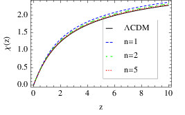
|
2.2 Stability Condition
Let us study the stability of the model by perturbatively expanding the action of the galileon field at second order as . We neglect the metric perturbation, then the quadratic action becomes
| (33) |
where
| (34) | |||||
| (35) | |||||
To avoid ghost and instability, we require and , respectively. One of the attractor solution, , has obviously ghostly perturbation since in our model. Using the attractor condition (17), , , and can be written in terms of and as
| (36) | |||||
| (37) | |||||
| (38) |
Throughout the evolution of the universe, the matter density parameter is always less than unity, therefore, we require to avoid ghost instability, . In figure 2, the evolution of the sound speed of perturbations is plotted. The asymptotic behavior of the sound speed is given by
It is worthy to note the fact that the sound speed of the galileon field perturbation becomes zero for . In section 4, we show that the linear cosmological perturbation reduces to that of the model. In a case of large but finite value of , the time-dependence of the galileon field perturbation will become important even on sub-horizon scales. For a case of small value of , e.g., , we can use the quasi-static approximation safely on small scales, which is demonstrated in section 4.

3 Constraint from Supernovae and CMB distance Observation
The SCP Union2 Compilation is a collection of 557 type Ia supernovae data whose range of the redshift is [72]. The distance modulus, which is the difference between apparent and absolute magnitude of the object, is given by
| (42) |
where is the luminosity distance,
| (43) |
The best-fit value of the present matter density and can be determined by defined by
| (44) |
where , , and are the redshift, the distance modulus, and the error of the -th observed Ia SN. The left panel of figure 3 shows the confidence contour of on the plane and for the kinetic braiding model. We find the minimum of the is respectively given by for CDM model and for the kinetic braiding model with . The kinetic braiding model with requires the higher matter density parameter. A similar result is found in a recent paper [43].


|
The Wilkinson microwave background anisotropy (WMAP) observation also provide a constraint that relies on the distance to the last scattering surface. We here adopt the method using the shift parameter , the acoustic scale , and the redshift of the decoupling epoch [73]. In the spatially flat universe, the acoustic scale and the shift parameter are written and , respectively, where is the comoving distance and is the comoving sound horizon at the decoupling epoch [74]. Then, we define the chi squared (see [4, 43] for details)
| (45) |
where , , and the inverse covariance matrix
In this analysis, we adopted . The right panel of figure 3 shows and confidence contours of . Our result is consistent with [43] for the case . The higher models better match the CMB distance observation.
4 Linear Cosmological Perturbations
In this section, we consider the linear evolution of cosmological perturbations. Hereafter, we consider the era after the matter domination. The metric perturbation in the conformal Newtonian gauge is given by
| (50) |
We write the perturbation of the galileon field by . Hereafter, means . In appendix A, we summarized the perturbation equations in the general case. In our model, (14) and (15), the following equations are obtained.
The component of the Einstein equation yields
| (51) |
where we defined
| (52) |
and is the matter density perturbation. The component of the Einstein equation yields
| (53) |
and
| (54) |
The component yields
| (55) |
where describes the velocity field (see appendix A). The perturbed equation for the galileon field becomes
| (56) |
The perturbed equation for the matter component is described in appendix A. Instead of solving the evolution equation of the matter perturbation, we use the following equation [34], which is obtained by combining eqs. (51) and (55),
| (57) | |||||
where is the gauge invariant matter density contrast.
4.1 Limit of
In section 3, we showed that the background expansion of the kinetic braiding model approaches that of the CDM model as becomes large. In this subsection, we show that the linear cosmological perturbation of the kinetic braiding model also reduces to that of the cosmological constant model for .
From the attractor condition (17), in the limit of , we find that is constant,
| (58) |
In this case, the leading term expanded eq. (56) in terms of gives
| (59) |
where we used (54) and . Then, the solution of (59) is , where is an integration constant, which is determined by initial condition of and . This solution is the decaying solution, therefore, one can set . In the case , the galileon field perturbations in the right hand sides of eqs. (53) and (55) disappear, and the equations reduce to those of the model. The evolution equations of the matter perturbations are not altered unless the gravitational potentials are altered. We are considering the initial conditions that is the same as the CDM model. These suggest that the linear perturbations of the kinetic gravity braiding model for are equivalent to those of the CDM model. In our numerical computation, we have confirmed that the cosmological perturbations of the kinetic braiding model with large approach the result of the CDM model (see also subsection 4.2).
This property that our model reduces to the cosmological constant model can be understood in the Lagrangian (1) with eqs. (14) and (15). In the case, and , and in the Lagrangian are constants, then the term can be written as the total derivative, which can be dropped effectively when deriving the equation of motion. The term plays a role of the cosmological constant, and the kinetic braiding model reduces to the cosmological constant model for . This feature could be related to the fact that the sound speed of perturbations of the galileon field for is zero over the whole history of the universe. The perturbations of the galileon field can not propagate and does not induce an additional effect on gravity.
The feature that the linear perturbations of the kinetic braiding model approaches those of the cosmological constant model appears for very large , e.g., , as will be shown in the next subsection. Such a behavior of large model is different from that of smaller model, e.g., . For the case , the quasi-static approximation can be adopted for the galileon field perturbations on the subhorizon scales, while it is not valid for . This comes from the behavior of the sound speed of the galileon field perturbations. In the k-essence model with a zero sound speed, the scalar field perturbations cluster, and enhance the cosmological perturbations [75], which is a contrast to our kinetic braiding model on the attractor solution (17).
4.2 Numerical Calculation
In this subsection, we show the evolution of the perturbations solved numerically. In figure 5, we plotted the evolutions of the gravitational potential (upper left panel), the perturbations of the galileon field (upper right panel), and the density perturbations (lower panel), for the kinetic braiding model with with adopting different wavenumbers labeled there and for the model. Figs. 5, 6 and 7 are the same as figure 5 but with , and , respectively. We can see that the perturbations approach those of the model as becomes large, as we discussed in subsection 4.1. For , the perturbations and with are almost the same as those of the CDM model, as one can see from figure 7. Since the sound speed of the perturbed galileon field become smaller as increases, longer wavelength perturbations with larger are not affected by the galileon field. Thus, the longer wavelength perturbations approach the model quickly as increases.
Let us discuss about the choice of the initial condition of the numerical computation. For the galileon field perturbations, the above results adopted the initial conditions and , where the subscript denotes the initial values at . In the Galileon scalar-tensor models [34], it has been pointed out that a different choice of the initial condition might give rise to an oscillating behavior in , , and . Figs. 8, 9 and 10 compares the gravitational potential , the perturbation of the galileon field , and the growth factor , as a function of the scale factor, for the kinetic braiding model with the different initial conditions , , and , respectively, where the other parameters are the same as those of Fig. 5. The behavior of the cosmological perturbations and are almost same for as long as . The difference becomes smaller as the initial value is smaller. Even for the cases and , the the difference appears only for the large scales . We also checked that the different choice of does not alter this conclusion as long as , where is the Hubble parameter at the initial time . Therefore, the result is not very sensitive to the choice of the initial condition within a suitable range of it.
If we assume that the galileon field undergoes an inflationary period at the early stage of the universe, fluctuations of order could be set, where is the Hubble scale determined by the energy scale of the inflation. The condition yields , which might be satisfied as long as the energy scale of the inflation is not so high.
For the model with larger , the quasi-static approximation for the galileon field perturbation fails. We can estimate the condition for the validity of the quasi-static approximation, as follows. From the equation of motion obtained from (33), the condition is given by . Using the relations and , the quasi-static approximation is valid as long as . We find that the quasi-static approximation is valid for the wavenumber for from numerical results. However, the quasi-static approximation no longer works for . This is because the sound speed of perturbations of the galileon field approaches zero for very large .


|


|


|

|


|

|


|

|


|


|


|


|


|


|
4.3 Quasi-Static Approximation
Hereafter, we consider the model with , in which small-scale perturbation equations can be expressed in simple forms by using the quasi-static and the sub-horizon approximation. Neglecting the time-derivative terms of perturbations and assuming that the wavelength of perturbation is well inside the Hubble horizon, , the evolution equation for the matter overdensity in linear theory reduces to
| (60) |
where we used the fact (see also appendix A). From eqs. (53) and (54), we have
| (61) |
where we introduced . From eq. (56), we have
| (62) |
for the galileon field perturbation. Combining (61) and (62), we obtain the modified Poisson equation,
| (63) |
where the effective gravitational constant is given by
| (64) | |||||
Here, in the second line, we used the attractor condition (17). Then, the evolution equation for the matter overdensity in linear theory can be written as
| (65) |
The crucial difference between the kinetic braiding model and the scalar-tensor galileon theory [33, 34, 35] is the absence of an effective anisotropic stress in the right-hand-side of eq. (54). The effective gravitational constant is nearly equal to at early times and becomes larger than at late times. (See the dashed curve in the right panel of figure 17). The enhancement of the effective gravitational constant leads to an enhancement of the growth factor of matter density perturbations. Although the background evolution for large approaches the model, the growth history is different due to the time-dependent effective gravitational constant. The left panel of figure 11 compares the evolution of the growth factor divided by the scale factor, , which is normalized as at early stage of the evolution. The growth factor of the kinetic braiding model is larger than that of the model throughout its growth history. In the right panel of figure 11, the linear growth rate is plotted.


|
4.4 Analytic Formula for Growth Index
The growth rate can be parametrized by the growth index defined by . It has been known that the growth rate of the model is well approximated by the nearly constant value . This parametrization was first introduced in [76] and has the potential to distinguish dark energy models and modified gravity models [77]. In this section, we derive the analytic formula of the growth index for the kinetic braiding model. As we will show below, the behavior of the growth index is unique in the kinetic braiding model, which will be important to distinguish between the kinetic braiding model and the model when is not infinite.
The matter evolution equation (65) can be written in terms of the growth rate as
| (66) |
By using the background equation and (17) , we have
| (67) | |||||
| (68) |
Using eqs. (64), (67) and (68), eq. (66) can be written as
| (69) |
We assume that the growth index can be approximated in the following expanded form,
| (70) |
Then, we expand eq. (69) around and we have the asymptotic value of the growth index at high redshift,
| (71) |
The higher order coefficients can be easily found. By way of example, table 1 summarizes the coefficients for the model and . The redshift evolution of is important in the kinetic braiding model. This is shown in figure 12, which plots the growth index , by solving eq. (66) numerically, as a function of redshift, for and , respectively. Figure 13 compares the numerical result and the approximate formula of (70) of the model as a function of redshift. The left panel of figure 13 plots the numerical result and the approximate formula with and , respectively, where is the maximum index in (70). The right panel shows the relative error for and . The approximate formula (70) with reproduces the exact growth rate to better than , and the growth factor can be obtained in a highly accurate manner, by . For the other case in table 1, we have the similar result and confirmed that the growth factor can be well approximated by the formula up to .


|
| 0.48529 | 0.46154 | 0.45316 | 0.44895 | 0.44643 | |
| -0.03373 | -0.03153 | -0.02922 | -0.02791 | -0.02708 | |
| -0.02814 | -0.02037 | -0.01876 | -0.01805 | -0.01764 | |
| -0.01667 | -0.01470 | -0.01393 | -0.01355 | -0.01333 | |
| -0.01367 | -0.01174 | -0.01119 | -0.01093 | -0.01078 | |
| -0.01106 | -0.00976 | -0.00936 | -0.00916 | -0.00905 |
On very small scales, the non-linear terms of become more important than metric perturbations in the case of small . The field equation for the galileon field including the non-linear terms is given by
| (72) |
which holds for the general Lagrangian (1) as long as the quasi-static approximation works. The equations for the metric perturbation remain the same as those of the linear perturbation theory. From eq. (72), the non-linear terms in the galileon field equation become dominant when . From eq. (62), we may estimate , by using the relation, . Combining these relations, the non-linear terms become dominant when . Therefore, for , we need to take into account the non-linear terms, and these terms play an important role in the Vainshtein mechanism as we will see in section 6.
In the limit of , the linear cosmological perturbation approaches the CDM model. It would be interesting to clarify what is the nature of the gravity in the model with large on the small scales where the Vainshtein mechanism works in the static limit. However, this is outside of the scope of the present paper, and we only consider the case in the latter part of this paper.
5 Cosmological Constraints from the Redshift-space Distortion
5.1 Current Constraint
The multipole power spectrum is useful for measuring the redshift-space distortion, which plays a vital role of testing gravity on the scales of cosmology [78, 79, 80, 81, 82, 83]. In this section, utilizing the monopole and quadrupole spectra from the SDSS LRG sample of the data release 7 [84, 31], we investigate a constraint on the kinetic braiding model. The multipole power spectrum is defined by
| (73) |
where the redshift-space power spectrum, are the Legendre polynomials, is the directional cosine between the line of sight direction and the wavenumber vector. The monopole represents the angular averaged power spectrum, and is the quadrupole spectrum which gives the leading anisotropic contribution. For the theoretical modeling of the redshift-space power spectrum, we adopt the fitting formulas developed by Jennings et al. [85] and Peacock and Dodds [86], with the transfer function by Eisenstein and Hu [87]. We consider the galaxy redshift-space power spectrum [88],
| (74) |
where is the nonlinear matter power spectrum, is the power spectrum of the velocity divergence, and is the cross power spectrum of matter and the velocity divergence, is the clustering bias, and is the velocity dispersion. Jennings et al. proposed a fitting formula for the redshift-space power spectrum of the form (74), assuming . The fitting formula relates the nonlinear matter power spectrum to and . Although the accuracy of the fitting formula for the kinetic braiding modified model is not verified, we assume its validity, and use it in this section. Also we consider the scale dependent bias in the form,
| (75) |
where , , and are the free parameters. The multipole power spectrum is measured assuming the fiducial distance-redshift relation of the spatially flat CDM model with =0.28. In order to compare the theoretical prediction of the kinetic braiding model with the observed power spectrum, we must take the cosmological redshift-space distortion into account [89]. Denoting the comoving distance and redshift relation of the kinetic braiding model, , the galaxy power spectrum with the cosmological redshift-space distortion is
| (76) |
where we defined , , and we use the mean redshift of the SDSS LRG sample.
We use the monopole and quadrupole power spectra in the range of wavenumber, , and compute the chi squared,
| (77) |
where is the observed power spectrum and is the covariance matrix. and are from refs. [84], which used luminous red galaxy sample of the Sloan Digital Sky survey data release 7 with the contiguous part of sky coverage in the redshift range , and the corresponding mock catalogues.
Figure 14 shows the contours on the plane for the model (upper left panel) and for the kinetic braiding model with (upper right panel), (lower left panel) and (lower right panel), respectively. In each panel, the and confidence contour-levels are given by dashed curve and solid curve, respectively. In the analysis, we fixed the spectral index and the density parameter for baryon , and the is computed to minimize (77) by fitting the bias parameters , , and the velocity dispersion . In this figure, we may understand that the constraint on comes from the baryon acoustic oscillation feature, and the constraint on comes from the amplitude of the monopole and the quadrupole spectrum. From figure 14, the kinetic braiding model with smaller favors the smaller values of and , compared with the model. However, the difference is not quite large, and the constraint is not very tight.
Our result is obtained by extrapolating the quasi-nonlinear formula to the kinetic braiding model. The Vainshtein mechanism is important on small scales in the kinetic braiding model, as in the case of the DGP model [90, 91, 92]. In the present paper, however, we neglect the nonlinear Vainshtein effect because we need to consider only rather large scales, . But, the validity will be necessary to be checked using N-body simulations in future.


|


|
5.2 Future Prospect
We now consider a future prospect constraining the kinetic braiding model using the multipole power spectra. Let us consider a redshift survey like the SuMIRe (SUbaru Measurement of Imaging and REdshift of the universe) PFS (Prime Focus Spectrograph) survey [93], which assumes the survey parameters like those of the WFMOS survey [94]. In the SuMIRe PFS survey, we assume the sky coverage is over redshift range with the averaged number density of galaxy .
Figure 15 shows the monopole (upper panels) and quadrupole (lower panels) power spectra multiplied by , and for the fiducial model with , and for the kinetic braiding model with , and . Here, we fixed . The left panels assume the subsample of the the range of redshift , while the right panels assume the subsample of the range redshift . The theoretical modeling of the power spectrum is the same as that in the above subsection, which is evaluated at the mean redshift of each subsample. In computing the theoretical power spectrum, we fixed the initial amplitude of the fluctuation so that the matter power spectrum of the model gives . Other cosmological parameters are fixed as and . The cosmological redshift-space distortion is taken in the power spectrum of the kinetic braiding model into account, assuming that the distance-redshift relation of the model is adopted in data analysis. The error bars for the model is evaluated by [95]
| (78) |
where is the volume of a shell in the Fourier space, and is the survey volume, , where is the survey area, and and are the maximum and minimum redshifts of the survey, respectively.
As for the bias , We adopted the scale-independent bias and the velocity dispersion for the model, but the scale-dependent bias (75) for the kinetic braiding model. In computing the power spectrum of kinetic braiding model, we assumed and as free parameters which are determined so as to minimize the value
| (79) |
where and are the power spectrum of the CDM model and the kinetic braiding model, and we used .
Figure 15 shows that the monopole spectrum can be almost same in the different models because of the bias, but the quadrupole spectrum is different. Thus, the combination of the monopole and quadrupole power spectra is useful to distinguish between the CDM model and the kinetic braiding model, depending on the model parameters. In 5.3, we estimates a constraint on and at a future quantitative level with the Fisher matrix analysis.

5.3 Fisher Matrix Analysis
In this subsection, let us discuss the future prospect of a constraint with galaxy power spectrum quantitatively using Fisher matrix analysis. We adopt the following Fisher matrix, for simplicity,
where is a survey volume, is a mean number density of galaxies, denotes a model parameter. In this Fisher matrix analysis, we consider the 6 parameters , , , , and . The amplitude of the initial cosmological perturbation is fixed so that for the CDM model. We also fixed the spectral index and . The curves in figure 16 show the 1-sigma (dashed curve) and 2-sigma (solid curve) confidence contours in the and plane, by marginalizing the Fisher matrix of the 6 parameters, , , , , and over the parameters other than and . In figure 16, we assumed the redshift survey like WFMOS/SuMIRe PFS survey, adopted in the previous subsection. The sky coverage is , the minimum and the maximum redshifts are and , respectively, and the averaged number density of galaxy is . The target model is the kinetic braiding model with , , , , , and . We assumed that the power spectrum is measured adopting the fiducial distance-redshift relation of the spatially flat CDM model with =0.28.
Figure 16 implies that the constraint on is tight, while the constraint on is not very tight. However, the 1-sigma (2-sigma) error in determining is () when the target parameter is . Then, it is possible to distinguish between the kinetic braiding model and the CDM model if . However, the constraint on becomes weaker when the target value of becomes large, since the background expansion and cosmological perturbations in the kinetic braiding model for is almost the same as the model. Then, it will be difficult to distinguish between the CDM model and the kinetic braiding model by a measurement of the redshift-space power spectrum when is large.

6 Non-linear Density Perturbation
In this section, we investigate the nonlinear effect of the perturbed galileon field on small scales. As discussed at the end of section 4, the non-linear term in the perturbed galileon field equation (72) becomes important for . Therefore, when considering the non-linear cosmological perturbations, we need to solve eq. (72). However, it is not easy to solve eq. (72) in general. For simplicity, we assume that the density perturbation has a spherically symmetric distribution and a top-hat profile. Then, the perturbation equation for the galileon field can be solved analytically, and it gives a qualitative picture of the Vainshtein mechanism in the kinetic braiding model. Note that eq. (72) is identical to the equation for the brane bending mode in the DGP model [96, 97, 91] and the full profile of the brane bending mode is investigated in [98]. The behavior of in a top-hat density profile remains the same in the kinetic braiding model.
We start with recasting the Poisson equation (63) and the field equation (72) by replacing the comoving nabla operator with the physical nabla operator, then we have
| (81) | |||
| (82) |
where we defined
| (83) |
As we will show below, the following combinations are useful,
| (84) | |||
| (85) |
Under the assumption that the density perturbation is spherically symmetric, the field equation (81) can be written as
| (86) |
Then, we define the enclosed mass perturbation, . Integrating eq. (86) over , we have
| (87) |
Solving for , we have
| (88) |
where and the Vainshtein radius of the enclosed mass is
| (89) |
Practically, eq. (87) yields two branches of solutions, which correspond to the attractive and repulsive force. We require that the solution matches the linear solution, given by at , hence we pick the solution whose value vanishes at an infinite distance. The Vainshtein radius for a point source can be estimated using eq. (89) and (17),
| (90) | |||||
where is the Schwartzschild radius of the point mass. Using the present values of and for , the Vainshtein radius is approximated by . The asymptotic behavior of the galileon field well inside and outside the Vainshtein radius is
respectively. Well outside the Vainshtein radius, , is proportional to the Newtonian potential and this solution corresponds to the linear solution. On the other hand, well inside the Vainshtein radius, , the galileon field approaches nearly constant [98] and does not contribute to the modified Poisson equation (82).
6.1 Top-Hat Profile
Hereafter, we consider the following top-hat density profile or, equivalently, the mass perturbation
We neglect any compensation underdensity swept out by the prior evolution of the top hat, and assume that a density enhancement is constant. For , is proportional to . Then, the non-linear term in eq. (81) can be written as
| (100) |
Therefore, eq. (81) can be written as
| (101) |
Setting and solving for , we have
| (102) |
where . Then, the modified Poisson equation (63) becomes
| (103) |
where the non-linear effective gravitational constant is given by
| (104) |
The first term of the right-hand-side of eq. (104) is the contribution from the Newtonian gravity and the second term induces the additional attractive force due to the perturbed galileon field. In the case , corresponding to , the effective gravitational constant approaches the standard gravitational constant and this is the Vainshtein mechanism in the spherical collapse in the cosmological perturbations (See the solid curve in the right panel of figure 17).
6.2 Spherical Collapse
In this section, we examine the spherical collapse which is a powerful tool for understanding the formation of a bound system in non-linear regime [99, 100, 101, 102, 103, 104]. The evolution of a spherical collapse undergoes three phases: (i) turn around, (ii) collapse, and (iii) virialization. A spherical overdense region expands along the expansion of the universe up to the maximum radius as the density perturbation evolves proportionally to the scale factor at early times. Then, it starts to shrink toward the center of the spherical region and finally collapses. The spherical collapse approach enables us to evaluate the critical density contrast and the virial density , which need in predicting the mass function of the halos. We assume that perturbed matter distribution remains a top-hat profile and each shell does not cross during collapse.
We start with the fully non-linear evolution equation for the matter over-density, which can be obtained from the energy-momentum conservation,
| (105) |
We assume that the total mass inside is conserved during collapse,
| (106) |
Differentiating eq. (106) with respect to time gives
| (107) |
Combining (105) and (106), the evolution equation for the spherical collapse is given by
| (108) | |||||
where we used (104) in the second line. For convenience, we rewrite the equation of motion as
| (109) |
where we have defined the gravitational potential contributed from the effective background term and from the effective gravitational constant .
6.3 Virial Theorem
For a spherically symmetric top-hat model, the total potential energy from the effective background term and the gravity is given by
| (110) |
where the potential energy of the gravity and the effective background term are
| (111) | |||
| (112) |
respectively. The virial theorem can be obtained by integrating the Boltzmann equation over all position, which gives . The virial radius is usually calculated by requiring the energy conservation at turnaround and virialization. However, there is the energy non-conservation problem in the dark energy models, DGP and other modified gravity models [98, 105]. The violation of energy conservation also arises in the kinetic braiding model due to the time-varying and . Hence, we need carefully choose the condition for the virialization epoch. In the present paper, we follow the approach in [98]. We choose the virialization epoch so that the virial condition satisfied, , where the kinetic energy during collapse can be computed by
| (113) |
We define the virial radius as the radius at the virialization epoch. The virial density is given by
| (114) |
where is the density at the virialization epoch and is the background matter density at the time of collapse.
We are now ready to solve the spherical collapse eq. (108), numerically. The total mass conservation within gives
| (115) |
where is the initial radius of the perturbation, is the initial density fluctuation, and is the initial scale factor. We set the initial scale factor . Turnaround and collapse are, respectively, defined by and . The left panel of figure 17 shows the evolution of the scaled radius for the and the kinetic braiding model with and . We set the initial density perturbation for the so that collapse occurs at . For the same initial density perturbation , the spherical overdensity region collapses earlier in the kinetic braiding model compared with the model due to the additional attractive force. The right panel of figure 17 shows the linear and non-linear effective gravitational constant as a function of redshift. The radius of the overdensity region enters the Vainshtein radius around for the case , and approaches the standard gravitational constant in the kinetic braiding model. Thus, the non-linear effect restores the general relativity in high density regions through the Vainshtein mechanism. Figure 18 shows the evolution of the critical density contrast and the virial density as a function of redshift. The critical density contrast is the value of the linear-theory density contrast reached to infinite density when the nonlinear top-hat perturbation collapses. One can see that for the kinetic braiding model approaches that of the Einstein de Sitter universe, , at high redshift. The virial density for the kinetic braiding model also approaches the value for Einstein de Sitter universe, , at high redshift. This is because the evolution of background and cosmological perturbations in the kinetic braiding model is identical to that in Einstein de Sitter universe at early times. Table 2 shows the numerical results of the critical density contrast and the virial density at for the model and the kinetic braiding model with and .
| 1.675 | 1.696 | 1.705 | 1.708 | 1.710 | 1.711 | |
| 360.4 | 305.8 | 306.2 | 306.3 | 306.3 | 306.4 |


|


|
6.4 Galaxy Cluster Counts
We here give a simple prediction about the mass function of halos by using the Press-Schechter formalism [106]. The number density of virialized clusters in an unit mass range as a function of redshift is given by
| (116) |
where , and is
| (117) |
with the top-hat smoothing function and the linear matter power spectrum at the redshift . The number count of halos in unit redshift within the range of mass, , is given by integrating the halo mass function,
| (118) |
where is the comoving volume of the unit redshift and is the survey area.
We consider the expected redshift distributions of clusters in the upcoming survey, the Southern Polar Telescope (SPT) Sunyaev Zeldovich (SZ) survey with a limiting flux density of at and a sky coverage of . The relation between the limiting flux and halo mass in the SPT survey [107] is given by
| (119) |
where is the angular diameter distance. In figure 19, we show the expected redshift distributions of clusters in the SPT survey in redshift bins of including Poisson errors for clusters above the limiting halo mass , which is determined by eq. (119). In the left panel, we compare the model and the kinetic braiding model with , where we fixed , and adopted for the model and and , respectively, for the kinetic braiding model. In the right panel, we compare the model and the kinetic braiding model with and , and , respectively, in which we fixed the initial amplitude of the power spectrum for the kinetic braiding model so that for the model.
As demonstrated in figure 19, the redshift distribution of the high-redshift clusters is practically useful to distinguish between the CDM model and the kinetic braiding model, depending on the cosmological parameters and the model parameters. However, figure 19 also demonstrates that the degeneracy between , and is problematic. Therefore, in order to distinguish between the CDM model and the kinetic braiding model, we need an independent constraint on the amplitude of the perturbations on the kinetic braiding model. This will be obtained by combining a measurement of the cosmic microwave background anisotropies or a measurement of the cosmic shear statistics from weak lensing surveys. The Fisher matrix analysis in section 6.5 estimates a constraint on and , assuming the amplitude of the cosmological perturbation can be determined from those independent observations.


|
6.5 Fisher Matrix Analysis
In this subsection, we investigate a constraint from the SPT survey predicted with the Fisher matrix analysis. The Fisher matrix for the cluster counts (e.g., [109]) can be written as
| (120) |
where is the number of galaxy clusters in the th redshift bin of the range ,
| (121) |
In the Fisher matrix analysis for the cluster counts, we consider 2 parameters, and , and adopt the target parameter and . The other cosmological parameters are fixed as those in section 5.3.
Figure 20 shows the 1-sigma (dashed curve) and 2-sigma (solid curve) confidence contours in the and plane, assuming like the SPT survey whose sky coverage is and the limiting flux, as explained in the previous section. From figure 20 one can see the similar feature as that in figure 16. The constraint on is not very tight. However, the 1-sigma (2-sigma) error in determining is () when . Thus, it is possible to distinguish between the kinetic braiding model and the CDM model if . However, the constraint on the model parameter become very weak when the target value of becomes large because the kinetic braiding model approaches the CDM model.

7 Conclusion
In this paper, we studied the cosmological consequences of the kinetic braiding model, whose self-interaction term is in the form, . This model allows the existence of a self-accelerating solution without ghost and instability for perturbations. Due to the Vainshtein mechanism, general relativity recovers on small scales, which ensures the consistency with the solar system tests. In this model with assuming the attractor condition (17), we found that the background evolution is identical to that of the Dvali-Turner’s model, which approaches the for equal to infinity. We also found that the linear growth history of the cosmological perturbation is identical to that of the model for . Using the Ia supernovae data [72] and the WMAP CMB data [4], we obtained a constraint on the model parameters of the kinetic braiding model. The kinetic braiding model with requires rather high matter density parameter, which is consistent with the result of [43]. We found the model with the higher can be consistent with the observations. We also found that the sound velocity of the galileon field perturbation becomes zero for . This prevents the perturbation of the galileon field from propagating, which breaks the quasi-static approximation when is large.
By solving the full equations of the linear cosmological perturbations numerically, we confirmed that the quasi-static approximation can be used for sub-horizon modes as long as . We investigated the evolution of the linear density perturbations as well as the spherical collapse in the nonlinear regime of the density perturbations, which are important in order to distinguish between the kinetic braiding model and the CDM model when is small. We also found a useful analytic expression for the growth index, in a form expanded in terms of the matter density parameter. The theoretical prediction for the large scale structure is confronted with the multipole power spectrum of the luminous red galaxy sample of the Sloan Digital Sky survey. The current constraint is not very tight, but a future redshift survey like the WFMOS/SuMIRe PFS survey would be potentially useful to distinguish between the kinetic braiding model and the CDM model if is small.
Based on the quasi-static approximation and the sub-horizon approximation for model , we also investigated the non-linear evolution of density perturbations using the spherical collapse, where the nonlinear effect of the galileon field perturbation plays an important role through the Vainshtein mechanism. We showed that the effective gravitational constant in the perturbation including the nonlinear effect approaches the usual Newton’s constant after the density becomes high. We also investigated a prospect for the number count of galaxy clusters in the SPT survey, which will be a useful test by combining other measurements like the cosmic microwave background anisotropies or the cosmic shear statistics of weak lensing surveys.
The kinetic braiding model in the present paper reduces to the CDM model for , which we demonstrated at least as for the background expansion and the linear cosmological perturbations. In this meaning, the kinetic gravity braiding can be unbraided by taking a large value of . This is an interesting feature that might be useful to understand the origin of the cosmological constant.
Acknowledgements.
This work was supported by Japan Society for Promotion of Science (JSPS) Grants-in-Aid for Scientific Research (Nos. 21540270, 21244033). This work is also supported by JSPS Core-to-Core Program “International Research Network for Dark Energy”. We thank K. Koyama, T. Yano, G. Nakamura, T. Narikawa, K. Ichiki, N. Sugiyama, A. Taruya, F. Schmidt, T. Kobayashi, and J. Soda for useful comments and discussions. We are grateful to I. Sawicki and his collaborators for useful comments on the investigation of the constraint from the CMB data. We also thank T. Sato and G. Huetsi for providing us with the data of the multipole power spectrum of the SDSS LRG sample. We also thank M. Sasaki, A. De Felice, S. Mukohyama and T. Takahashi for useful discussions.Appendix A Linear Perturbation Equations
In this appendix, we summarize perturbation equations for the general Lagrangian (1). The component of the Einstein equations is given by
| (122) |
where is defined by eq.(52) and is the matter density perturbation. The component of the Einstein equation is
| (123) | |||||
where describes the velocity field of the matter component (See below for details). The traceless part of the component of the Einstein equation gives (54), while the trace part yields
| (124) |
where is the perturbation of pressure. The perturbation equation for the galileon field is given by
| (125) |
Let us summarize the perturbations of the matter component, whose evolution equation is given by the energy-momentum conservation . The perturbation of the energy-momentum tensor is given by , , and , respectively. The energy-momentum conservation yields
| (126) | |||
| (127) |
For the matter perturbations, we can set . It is convenient to define the quantity . In terms of the density contrast and , these equations can be written as
| (128) | |||
| (129) |
Taking the time derivative of (129) and using (129), we obtain the evolution equation for the matter density perturbation,
| (130) |
Finally, we introduce the gauge-invariant density perturbation, , and the new variable, . Then, the matter perturbation obeys the following equation,
| (131) |
References
- (1) A. G. Riess et al., Observational Evidence from Supernovae for an Accelerating Universe and a Cosmological Constant, Astron. J. 116 (1998) 1009
- (2) S. Perlmutter et al., Measurements of Omega and Lambda from 42 High-Redshift Supernovae, Astropys. J. 517 (1999) 565
- (3) D. N. Spergel et al., Three-Year Wilkinson Microwave Anisotropy Probe (WMAP) Observations: Implications for Cosmology, Astropys. J. Suppl. 170 (2007) 377
- (4) E. Komatsu, et al.,Seven-year Wilkinson Microwave Anisotropy Probe (WMAP) Observations: Cosmological Interpretation, Astrophys. J. Suppl. 192 (2011) 18
- (5) B. Reid, et al., Cosmological constraints from the clustering of the Sloan Digital Sky Survey DR7 luminous red galaxies, Mon. Not. Roy. Astron. Soc. 404 (2010) 60
- (6) M. Tegmark et al., Cosmological constraints from the SDSS luminous red galaxies, Phys. Rev. D 74 (2006) 123507
- (7) K. Vanderlinde, et al., Galaxy Clusters Selected with the Sunyaev-Zel’dovich Effect from 2008 South Pole Telescope Observations, Astrophys. J. 722 (2010) 1180
- (8) D. Rapetti, S. W. Allen and J. Weller, Constraining dark energy with X-ray galaxy clusters, supernovae and the cosmic microwave background, Mon. Not. Roy. Astron. Soc. 360 (2005) 555
- (9) P. J. E. Peebles and B. Ratra, The cosmological constant and dark energy, Rev. Mod. Phys. 75 (2003) 559
- (10) T. Padmanabhan, Cosmological constant-the weight of the vacuum, Phys. Rept. 380 (2003) 235
- (11) S. Weinberg, The cosmological constant problem, Rev. Mod. Phys. 61 (1989) 1
- (12) S. Weinberg, The Cosmological Constant Problems, astro-ph/0005265
- (13) L. Amendola, Scaling solutions in general nonminimal coupling theories, Phys. Rev. D 60 (1999) 043501
- (14) J. P. Uzan, Cosmological scaling solutions of nonminimally coupled scalar fields, Phys. Rev. D 59 (1999) 123510
- (15) T. Chiba, Quintessence, the gravitational constant, and gravity, Phys. Rev. D 60 (1999) 083508
- (16) N. Bartolo and M. Pietroni, Scalar-tensor gravity and quintessence, Phys. Rev. D 61 (2000) 023518
- (17) F. Perrotta, C. Baccigalupi and S. Matarrese, Extended quintessence, Phys. Rev. D 61 (2000) 023507
- (18) S. M. Carroll, V. Duvvuri, M. Trodden and M. S. Turner, Is cosmic speed-up due to new gravitational physics?, Phys. Rev. D 70 (2004) 043528
- (19) S. Nojiri and S. D. Odintsov, Modified gravity with negative and positive powers of curvature: Unification of inflation and cosmic acceleration, Phys. Rev. D 68 (2003) 123512
- (20) S. Capozziello, S. Carloni and A. Troisi, Quintessence without scalar fields, Recent Res. Dev. Astron. Astrophys. 1 (2003) 625
- (21) W. Hu and I. Sawicki, Models of f(R) cosmic acceleration that evade solar system tests, Phys. Rev. D 76 (2007) 064004
- (22) A. A. Starobinsky, Disappearing cosmological constant in f(R) gravity, JETP Lett. 86 (2007) 157
- (23) S. Tsujikawa, Observational signatures of f(R) dark energy models that satisfy cosmological and local gravity constraints, Phys. Rev. D 77 (2008) 023507
- (24) S. Nojiri and S. Odintsov, Unifying inflation with ©CDM epoch in modified f(R) gravity consistent with Solar System tests, Phys. Lett. B 657 (2007) 238
- (25) G. R. Dvali, G. Gabadadze and M. Porrati, Metastable gravitons and infinite volume extra dimensions, Phys. Lett. B 484 (2000) 112
- (26) G. R. Dvali, G. Gabadadze and M. Porrati, 4D gravity on a brane in 5D Minkowski space, Phys. Lett. B 485 (2000) 208
- (27) Y-S. Song, I. Sawicki and W. Hu, Large-scale tests of the Dvali-Gabadadze-Porrati model, Phys. Rev. D 75 (2007) 064003
- (28) R. Maartens and E. Majerotto, Observational constraints on self-accelerating cosmology, Phys. Rev. D 74 (2006) 023004
- (29) R. Maartens and K. Koyama, Brane-World Gravity, Living Rev. Rel. 13 (2010) 5
- (30) F. Schmidt, A. Vikhlinin and W. Hu, Cluster constraints on f(R) gravity, Phys. Rev. D 80 (2009) 083505
- (31) K. Yamamoto, G. Nakamura, G. Hutsi, T. Narikawa and T. Sato, Constraint on the cosmological f(R) model from the multipole power spectrum of the SDSS luminous red galaxy sample and prospects for a future redshift survey, Phys. Rev. D 81 (2010) 103517
- (32) N. Chow and J. Khoury, Galileon cosmology, Phys. Rev. D 80 (2009) 024037
- (33) F. P. Silva and K. Koyama, Self-accelerating universe in Galileon cosmology, Phys. Rev. D 80 (2009) 121301
- (34) T. Kobayashi, H. Tashiro and D. Suzuki, Evolution of linear cosmological perturbations and its observational implications in Galileon-type modified gravity, Phys. Rev. D 81 (2010) 063513
- (35) T. Kobayashi, Cosmic expansion and growth histories in Galileon scalar-tensor models of dark energy, Phys. Rev. D 81 (2010) 103533
- (36) A. De Felice and S. Tsujikawa, Generalized Galileon cosmology, arXiv:1008.4236
- (37) A. De Felice and S. Tsujikawa, Generalized Brans-Dicke theories, JCAP 07 (2010) 024
- (38) A. De Felice, S. Mukohyama and S. Tsujikawa, Density perturbations in general modified gravitational theories, Phys. Rev. D 82 (2010) 023524
- (39) C. Deffayet, G. Esposito-Farese and A. Vikman, Covariant Galileon, Phys. Rev. D 79 (2009) 084003
- (40) R. Gannouji and M. Sami, Galileon gravity and its relevance to late time cosmic acceleration, Phys. Rev. D 82 (2010) 024011
- (41) A. Ali, R. Gannouji and M. Sami, Modified gravity a la Galileon: Late time cosmic acceleration and observational constraints, Phys. Rev. D 82 (2010) 103015
- (42) A. De Felice and S. Tsujikawa, Cosmology of a Covariant Galileon Field, Phys. Rev. Lett. 105 (2010) 111301
- (43) S. Nesseris, A. De Felice and S. Tsujikawa, Observational constraints on Galileon cosmology, Phys. Rev. D 82 (2010) 124054
- (44) D. F. Mota, M. Sandstad and T. Zlosnik, Cosmology of the selfaccelerating third order Galileon, arXiv:1009.6151
- (45) A. De Felice, R. Kase, S. Tsujikawa, Matter perturbations in Galileon cosmology, arXiv:1011.6132
- (46) C. Deffayet, O. Pujolas, I. Sawicki and A. Vikman, Imperfect dark energy from kinetic gravity braiding, JCAP 10 (2010) 026
- (47) C. Deffayet, S. Deser and G. Esposito-Farese, Generalized Galileons: All scalar models whose curved background extensions maintain second-order field equations and stress tensors, Phys. Rev. D 80 (2009) 064015
- (48) A. Nicolis, R. Rattazzi and E. Trincherini, Galileon as a local modification of gravity, Phys. Rev. D 79 (2009) 064036
- (49) C. Burrage and D. Seery, Revisiting fifth forces in the Galileon model, JCAP 08 (2010) 011
- (50) G. L. Goon, K. Hinterbichler and M. Trodden, Stability and superluminality of spherical DBI galileon solutions, arXiv:1008.4580
- (51) C. de Rham and A. J. Tolley, DBI and the Galileon reunited, JCAP 05 (2010) 015
- (52) A. Padilla, P. M. Saffin and S. Zhou, Bi-galileon theory I: motivation and formulation, JHEP 12 (2010) 031
- (53) A. Padilla, P. M. Saffin and S. Zhou, Bi-galileon theory II: phenomenology, arXiv:1008.3312
- (54) E. Dyer and K. Hinterbichler, Boundary terms and junction conditions for the DGP Pi-Lagrangian and galileon, JHEP 11 (2009) 059
- (55) A. Padilla, P. M. Saffin and S. Zhou, Multi-galileons, solitons and Derrick’s theorem, arXiv:1008.0745
- (56) K. Hinterbichler, M. Trodden and D. Wesley, Multifield Galileons and higher codimension branes, Phys. Rev. D 82 (2010) 124018
- (57) M. Andrews, K. Hinterbichler, J. Khoury and M. Trodden, Instabilities of Spherical Solutions with Multiple Galileons and SO(N) Symmetry, arXiv:1008.4128
- (58) C. Deffayet, S. Deser and G. Esposito-Farese, Arbitrary p-form Galileons, Phys. Rev. D 82 (2010) 061501
- (59) E. Babichev, Galileon accretion, arXiv:1009.2921
- (60) C. Burrage, C. de Rham, D. Seery and A. J. Tolley, Galileon inflation, JCAP 01 (2011) 014
- (61) T. Kobayashi, M. Yamaguchi and J. Yokoyama, Inflation Driven by the Galileon Field, Phys. Rev. Lett. 105 (2010) 231302
- (62) K. Kamada, T. Kobayashi, M. Yamaguchi, J. Yokoyama, Higgs G-inflation, arXiv:1012.4238
- (63) S. Mizuno and K. Koyama,Primordial non-Gaussianity from the DBI Galileons, Phys. Rev. 82 (2010) 103518
- (64) A. Nicolis and R. Rattazzi, Classical and Quantum Consistency of the DGP Model, JHEP 06 (2004) 059
- (65) M. A. Luty, M. Porrati and R. Rattazzi, Strong interactions and stability in the DGP model, JHEP 09 (2003) 029
- (66) A. I. Vainshtein, To the problem of nonvanishing gravitation mass, Phys. Lett. B 39 (1972) 393
- (67) G. Dvali and M. S. Turner, Dark energy as a modification of the Friedmann equation, astro-ph/0301510
- (68) K. Koyama, Structure formation in modified gravity models, JCAP 03 (2006) 017
- (69) J-P. Uzan, The acceleration of the universe and the physics behind it, astro-ph/0605313
- (70) K. Yamamoto, D. Parkinson, T. Hamana, R.C. Nichol and Y. Suto, Optimizing future imaging survey of galaxies to confront dark energy and modified gravity models, Phys. Rev. D 76 (2007) 023504 [Erratum ibid D 76 (2007) 129901]
- (71) K. Koyama and R. Maartens, Structure formation in the Dvali Gabadadze Porrati cosmological model, JCAP 01 (2006) 016
- (72) R. Amanullah et al., Spectra and Hubble Space Telescope Light Curves of Six Type Ia Supernovae at 0.511z1.12 and the Union2 Compilation, Astrophys. J. 716 (2010) 712
- (73) Y. Wang and P. Mukherjee, Observational constraints on dark energy and cosmic curvature, Phys. Rev. D 76 (2007) 103533
- (74) W. Hu and N. Sugiyama, Small-Scale Cosmological Perturbations: an Analytic Approach, Astrophys. J. 471 (1996) 542
- (75) P. Creminelli, G. D’Amico, J. Norena, L. Senatore, F. Vernizzi, Spherical collapse in quintessence models with zero speed of sound, JCAP 03 (2010) 027
- (76) P. J. E. Peebles, Large-Scale Structure of the Universe, Princeton University Press (1980)
- (77) E. V. Linder, Cosmic growth history and expansion history, Phys. Rev. D 72 (2005) 043529
- (78) E. V. Linder, Redshift distortions as a probe of gravity, Astropart. Phys. 29 (2008) 336
- (79) L. Guzzo et al., A test of the nature of cosmic acceleration using galaxy redshift distortions, Nature 451 (2008) 541
- (80) K. Yamamoto, T. Sato and G. Hütsi, Testing General Relativity with the Multipole Spectra of the SDSS Luminous Red Galaxies, Prog. Theor. Phys. 120 (2008) 609
- (81) M. White, Y. Song and W. J. Percival, Forecasting cosmological constraints from redshift surveys, Mon. Not. Roy. Astron. Soc. 397 (2009) 1348
- (82) R. Reyes, et al., Confirmation of general relativity on large scales from weak lensing and galaxy velocities, Nature 464 (2010) 256
- (83) K. Hirano, Observational tests of Galileon gravity with growth rate, arXiv:1012.5451
- (84) T. Sato, G. Hüetsi and K. Yamamoto, Deconvolution of Window Effect in Galaxy Power Spectrum Analysis, Prog. Theor. Phys. 125 (2011) 187
- (85) E. Jennings, C. M. Baugh and S. Pascoli, Modelling redshift space distortions in hierarchical cosmologies, Mon. Not. Roy. Astron. Soc. 410 (2010) 2081
- (86) J. A. Peacock and S. J. Dodds, Non-linear evolution of cosmological power spectra, Mon. Not. Roy. Astron. Soc. 280 (1996) L1
- (87) D. J. Eisenstein and W. Hu, Baryonic Features in the Matter Transfer Function, Astrophys. J. 496 (1998) 605
- (88) R. Scoccimarro, Redshift-space distortions, pairwise velocities, and nonlinearities, Phys. Rev. D 70 (2004) 083007
- (89) W. E. Ballinger, J. A. Peacock and A. F. Heavens, Measuring the cosmological constant with redshift surveys, Mon. Not. Roy. Astron. Soc. 282 (1996) 877
- (90) K. Koyama, A. Taruya and T. Hiramatsu, Nonlinear evolution of the matter power spectrum in modified theories of gravity, Phys. Rev. D 79 (2009) 123512
- (91) F. Schmidt, Cosmological simulations of normal-branch braneworld gravity, Phys. Rev. D 80 (2009) 123003
- (92) R. Scoccimarro, tLarge-scale structure in brane-induced gravity. I. Perturbation theory, Phys. Rev. D 80 (2009) 104006
- (93) H. Aihara, talk at the IPMU international conference on dark energy: lighting up the darkness!, Kashiwa, Japan, 2009
- (94) B. Bassett, R. C. Nichol and D. J. Eisenstein, WFMOS: Sounding the dark cosmos, Astronomy and Geophysics 46 (2005) 5.26
- (95) K. Yamamoto, M. Nakamichi, A. Kamino, B. A. Bassett and H. Nishioka, Measurement of the Quadrupole Power Spectrum in the Clustering of the 2dF QSO Survey, Publ. Astron. Soc. Japan 58 (2006) 93
- (96) K. Koyama and F. P. Silva, Nonlinear interactions in a cosmological background in the Dvali-Gabadadze-Porrati braneworld, Phys. Rev. D 75 (2007) 084040
- (97) A. Lue, R. Scoccimarro and G. D. Starkman, Probing Newton’s constant on vast scales: Dvali-Gabadadze-Porrati gravity, cosmic acceleration, and large scale structure, Phys. Rev. D 69 (2004) 124015
- (98) F. Schmidt, W. Hu and M. Lima, Spherical collapse and the halo model in braneworld gravity, Phys. Rev. D 81 (2010) 063005
- (99) J. E. Gunn and J. R. Gott, On the Infall of Matter Into Clusters of Galaxies and Some Effects on Their Evolution, Astrophys. J. 176 (1972) 1
- (100) O. Lahav, P. B. Lilje, J. R. Primack and M. J. Rees, Dynamical effects of the cosmological constant, Mon. Not. Roy. Astron. Soc. 251 (1991) 128
- (101) L. Wang and P. J. Steinhardt, Cluster Abundance Constraints for Cosmological Models with a Time-varying, Spatially Inhomogeneous Energy Component with Negative Pressure, Astrophys. J. 508 (1998) 483
- (102) C. Horellou and J. Berge, Dark energy and the evolution of spherical overdensities, Mon. Not. Roy. Astron. Soc. 360 (2005) 1393
- (103) S. Basilakos, J. C. B. Sanchez and L. Perivolaropoulos, Spherical collapse model and cluster formation beyond the © cosmology: Indications for a clustered dark energy?, Phys. Rev. D 80 (2009) 043530
- (104) M. Manera and D. F. Mota, Cluster number counts dependence on dark energy inhomogeneities and coupling to dark matter, Mon. Not. Roy. Astron. Soc. 371, (2006) 1373
- (105) I. Maor and O. Lahav, On virialization with dark energy, JCAP 07 (2005) 003
- (106) W. H. Press and P. Schechter, Formation of Galaxies and Clusters of Galaxies by Self-Similar Gravitational Condensation, Astrophys. J. 187 (1974) 425
- (107) C. Fedeli, L. Moscardini, and S. Matarrese, The clustering of galaxy clusters in cosmological models with non-Gaussian initial conditions: predictions for future surveys, Mon. Not. Roy. Astron. Soc. 397 (2009) 1125
- (108) K. Yamamoto, Optimal Weighting Scheme in Redshift-Space Power Spectrum Analysis and a Prospect for Measuring the Cosmic Equation of State, Astrophys. J. 595 (2003) 580
- (109) S. Wang, J. Khoury, Z.Haiman, Constraining the evolution of dark energy with a combination of galaxy cluster observables, Phys. Rev. D 70 (2004) 123008