Helical Edge Modes near Transition to Topological Insulator with Indirect Gap

Let us first consider a straight edge geometry (see Fig. 1a), in which electrons are confined to $N_{r}$ rows in a strip between $y=1$ and $y=N_{r}$, i.e., the two edges are along $x$-axis. Translational invariance along $x$-axis allows for constructing a 1D tight-binding Hamiltonian $h_{01}(k)$ with $k=k_{x}$ in terms of the creation $c^{\dagger}_{J}(k)$ and annihilation $c_{J}(k)$ operators with row index $J$, which are two-component vectors in the pseudo-spin space. For up spin, the 1D model $h_{\uparrow}$ is obtained as

where $\hat{\cal E}(k)$ and $\hat{t}_{y}$ are given by

Here and in the following, we use the notation $\Delta_{B}\equiv\Delta-4$. The corresponding Schrödinger equation is given by

where $\Psi_{J}$ is the two-component amplitude with row index $J$. The straight edges along the $J=1$ row and $J=N_{r}$ row can be implemented by open boundary condition $\Psi_{0}=\Psi_{N_{r}+1}=0$.

We consider the thermodynamic limit $N_{r}\rightarrow\infty$, and try an edge state solution with property: $\Psi_{J+1}=\lambda\Psi_{J}=\lambda^{J+1}\Psi$ with $|\lambda|<1$[18, 19]. Here $\lambda$ is a complex number in general. Then Eq.(15) can be written in the following form:

Although $P_{01}(\lambda,k)$ is a $2\times 2$ matrix, there is at most one solution $\Psi$ for the helical edge mode in Eq.(16). We decompose $P_{01}(\lambda,k)$ into the Hermitian part and the rest called the annihilator[16]. The absence of the particle-hole symmetry in the present case requires a little more complicated procedure than before [16]. Let us first introduce a parameter $\phi$ and make the following transformation:

Then, we have

Now we decompose $P_{01}(\lambda,k)$ in Eq.(16) as

where the Hermitian part $H_{01}$ is chosen as combination of $\sigma_{0}\ (=1)$ and $\sigma_{X}$ terms. The eigenstate $\Psi$ of $H_{01}$ obeys the relation $\sigma_{X}\Psi=s\Psi$ with $s=\pm 1$. Furthermore, $\sigma_{y}$ and $\sigma_{Z}$ terms combine to form the annihilator $F_{01}$ [16]. Namely we obtain

In view of $E(k)$ being real, and the parameter $\lambda$ being complex in general, we require in $H_{01}$ the condition

which determines $\phi$ as

Then $E(k)$ of the edge mode reads

The condition for $F_{01}$, which is given by Eq.(27), to form the annihilator $\sigma_{y}+is\sigma_{Z}$ reads

which determines $\lambda$ since $\phi$ has already been fixed by Eq.(29). The solutions $\lambda=\lambda_{s\pm}(k)$ are given by

with $\cos{\phi}=\sqrt{1-D^{2}}$. The dependence on $k$ comes only through ${\cal E}_{3}$. For complex $\lambda$, we obtain

which does not depend on $k$, and should be less than unity. Therefore, we must choose $s=1$ that corresponds to the right-going mode. We obtain the spectrum:

In the case of $D=0$, the spectrum is reduced to $A\sin k$, which was already obtained [14, 15, 16]. The constant term $-D\Delta$ can be canceled by the chemical potential. Then the zero mode occurs at $k=0$. Otherwise the zero mode has a finite momentum. The two-component wave function is given by

apart from the normalization factor. Hereafter we use notation $\lambda_{\pm}=\lambda_{1\pm}$, since only the case of $s=1$ is relevant.

Fig.2 (a) shows the spectrum of the system including both $h_{\uparrow}$ and $h_{\downarrow}$, i.e., two helical modes. The bulk spectrum is obtained by projecting the 2D spectrum for a finite but large system into 1D BZ of the straight edge. The parameter $|\lambda_{\pm}|$ is shown in Fig.2 (b). The edge modes are present only if $|\lambda|<1$ is satisfied for both $\lambda_{\pm}$. It is clear from Fig.2(b) that the momentum range for the edge mode is split into two; one is localized around center of BZ, and the other allows for a reentrant edge mode [15, 16].

Furthermore, the two parts have exactly the same width for the momentum range. This fact can be understood by writing ${\cal E}_{3}$ in Eq.(22) as

with $\tan\alpha=2\sqrt{1-D^{2}}/(AD)$. This expression shows that ${\cal E}_{3}$ is symmetric about

which becomes $1.18$ with the chosen values of $A=1$ and $D=0.98$. Hence, according to Eq.(32), the value of $\lambda_{\pm}$ is also symmetric around $k_{c}$ as seen from Fig.2(b). The allowed momentum range for the edge mode with $|\lambda_{\pm}|<1$ is also symmetric around $k_{c}$.

Fig.3 shows the critical case with $D=1$ where the minimum value of conduction band is equal to the maximum value of valence band:

For the parameter $\lambda_{\pm}$, we obtain

which means $\lambda_{-}\leq-1$ for $0\leq k\leq\pi$, and $\lambda_{+}\geq 1$ for $-\pi\leq k\leq 0$. Therefore, the edge mode is absent for any momentum in the critical case.

For $D>1$, the bulk system becomes a semimetal. Fig.4 shows the spectrum in this case with $D=1.1$. Because we have $\sin{\phi}=-D<-1$, the edge mode is absent.

Let us summarize the situation with changing $D$ for the straight edge: With $D=0$, the system is topologically nontrivial insulator with particle-hole symmetry. For $D>0$, the particle-hole symmetry is broken and the shape of valence and conduction bands become different. As getting close to the critical case with $D=1$, the spectrum of the edge mode separates into two parts with the same width in the 1D momentum space, and both parts shrink simultaneously with further increase of $D$. At $D=1$, associated with closing of the bulk band gap, edge modes disappear in the whole BZ. With $D>1$, the system enters into semimetals where no edge modes are present for the straight edge.

We consider the edge mode in ordinary (topologically trivial) insulators (OI). In the particle-hole symmetric system, there is no edge modes [11, 14]. In the present case, edge modes can show up even in OI depending on the value of $D$. The presence of edge modes in OI can be analyzed conveniently by considering two limiting cases: (i) particle-hole symmetric case with $D=0$, where we obtain ${\cal E}_{3}=\Delta_{B}+2\cos{k}$; (ii) critical case with $D=1$, where the bulk energy gap closes and edge mode disappears. Here we obtain ${\cal E}_{3}=A\sin{k}$. In order to derive the momentum region allowing for edge modes, we consider extrema of $\lambda_{\pm}$ at $k=k_{c}$. We obtain from Eq.(37)

which is negative for

In the case of ${\cal E}_{3}<0$ we obtain $|\lambda_{+}(k_{c})|>|\lambda_{-}(k_{c})|$, and otherwise opposite inequality.

Fig.5 plots the parameters $|\lambda_{\pm}(k_{c})|$ given by Eq.(32) as a function of $D$. We set $\Delta=-1.2$, or $\Delta_{B}=-5.2$, which makes the system OI. Helical edge modes appear for $D_{c1}<D<1$ where the boundary $D_{c1}$ are given by solution of the condition

With $D$ increasing from zero to unity, $|\lambda_{+}(k_{c})|$ decreases, as seen in Fig 5. As long as $D<D_{c1}$, we have the relation $|\lambda_{+}(k_{c})|>1$, and no edge modes.

At $D=D_{c1}$, we obtain $|\lambda_{-}(k_{c})|<|\lambda_{+}(k_{c})|=1$, and the edge mode begins to show up. Fig.6 shows an example of the spectrum in the OI with $\Delta=-1.2$ and $A=1$. Here edge modes appear in the middle of the BZ without the reentrant behavior.

With further increase of $D$, we come close to the limiting case (ii), and have the reversed relation $|\lambda_{+}(k_{c})|<|\lambda_{-}(k_{c})|$. At $D=D_{c2}$, we obtain $|\lambda_{-}(k_{c})|=1$. Then the edge mode vanishes at $k=k_{c}$, but is still present on both sides of $k_{c}$. Thus, with $D_{c2}<D<1$, edge mode contains two separate parts. Fig.7 shows the spectrum and $|\lambda_{\pm}|$ corresponding to this case. The separate momentum regions, which are symmetric around $k_{c}$, shrink simultaneously until $D=1$ is reached, where edge modes disappear completely. In Fig.7 we obtain $k_{c}=1.307$ from Eq.(38).

Let us now consider the zigzag edge geometry, as illustrated in Fig.1(b). Electrons are confined in a diagonal strip: $1\leq y-x\leq N_{r}$, provided the edges are placed at $y-x=1$ and $y-x=N_{r}$, normal to the $(1,-1)$-direction. Translational invariance remains along the $(1,1)$-direction. Bulk energy $E_{\rm b}$ in terms of variables $\kappa=(k_{x}+k_{y})/2$ and $\xi=(k_{x}-k_{y})/2$ is obtained from Eq.(7) as

The Schrödinger equation for the edge mode analogous to Eq.(15) reads:

where

and we have introduced

Here the conserved momentum is $\kappa=(k_{x}+k_{y})/2$, with $-\pi/2<\kappa<\pi/2$. We impose the boundary condition: $\Phi_{0}=\Phi_{N_{r}+1}=0$ for zigzag edge geometry, and consider the thermodynamic limit $N_{r}\rightarrow\infty$.

Assuming eigenstate of Eq.(46) with property $\Phi_{j}=\lambda\Phi_{j-1}=\lambda^{j}\Phi$, where $|\lambda|<1$, we obtain

In order to construct the annihilator $F_{11}$ for the zigzag edge, we introduce further transformation:

Then, we have

We decompose $P_{11}$ in Eq.(50) as $P_{11}=H_{11}+F_{11}$ where

with

Note that $H_{11}$ contains non-Hermitian part due to the complex parameter $\lambda$. Since $H_{11}$ should have real eigenenergy $E_{\uparrow}(\kappa)$, we require the complex part in $H_{11}$ to be ineffective:

with $\sigma_{\theta x}\Phi=s\Phi$. Then the parameter $\theta$ is determined as

The eigenenergy is given by

where $s=+1$ should be chosen for the edge mode, as shown below. From Eq.(61) we obtain the limiting behavior:

which gives $E_{\uparrow}(0)=-D\Delta$ and $E_{\uparrow}(\pi/2)=-\Delta+4(1-D)$.

The corresponding annihilator $F_{11}$ in Eq.(56) should be proportional to $\sigma_{y}+is\sigma_{\theta z}$, which requires

with

The solution is given by

which leads, for complex $\lambda$, to

In order to choose the appropriate branch out of $s=\pm 1$, we put $\kappa=0$ and obtain $R=2\cos\theta>0$. In this case the quantity

is less than unity only with $s=+1$.

We now consider the case $\kappa=\pm\pi/2$. From Eq.(66) we obtain $R=A/\sqrt{2}$, and then

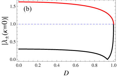
Since $\lambda_{s\pm}(\pm\pi/2)$ is complex, we obtain $|\lambda_{1\pm}|<1$ near the zone boundary. This property means that edge mode near zone boundary is stable against transition from TI to SM (or OI). However, its existent region shrinks with increasing $D$. Hereafter, we use notation $\lambda_{\pm}=\lambda_{1\pm}(\kappa)$.

In this subsection we fix $\Delta=\pm 1.2,A=1$, which realizes TI with $0<D<1$ and $\Delta>0$. Note that $\kappa=0$ is always a crossing point of two helical modes, as a result of time-reversal symmetry of the system. Hence this property is robust against particle-hole symmetry breaking as long as the system is still in TI. However, the existent regions of edge mode will shrink with increasing $D$.

Fig.8 shows the spectrum and $|\lambda_{\pm}|$ in the case of $D=0.9,\Delta=1.2$. As shown in the lower panel, we always have $|\lambda_{\pm}|<1$ for $0<\kappa<\pi/2$, which means the presence of the edge mode in the whole region of positive $\kappa$. With $\kappa<0$, there appears a reentrant edge mode near the zone boundary $\kappa=-\pi/2$, which is not seen in the upper panel because of its much lower energy. The binding energy of reentrant edge mode near zone boundary is expanded as

The reentrant mode merges with bulk excitations at momentum $\kappa_{m}$ that is given by the solution of

The analytic expression of $\kappa_{m}$ in terms of system parameters is complicated and it’s not illuminating. For the parameters used in Fig.8, we obtain the numerical value: $\kappa_{m}=-0.936\pi/2$. Since $\kappa_{m}$ is close to $-\pi/2$, the binding energy is only of the order of $10^{-3}$ according to Eq.(70). The reentrant mode vanishes also at the zone boundary because of the relation: $|\lambda_{\pm}|\rightarrow 1$ as $\kappa\rightarrow-\pi/2$.

In critical case with $D=1$, the bulk energy gap closes, with extremum of $E_{\rm b}$ given by

Fig.9 shows the spectrum and parameters $|\lambda_{\pm}|$ in this case. Since we obtain $|\lambda_{\pm}(\kappa=0)|=1$ with $D=1$, the crossing point of two helical edge modes merges with bulk excitations associated with indirect gap-closing, However, edge mode still exists in the other momentum region with $|\lambda_{\pm}|<1$. Note that the right-going helical mode has the flat spectrum for $\kappa>0$, and that the left-going helical mode has the flat spectrum for $\kappa<0$,

With $D>1$, the system is no longer a topological insulator. However the edge mode still survives in some momentum region. Fig.10 shows the spectrum and parameters $|\lambda_{\pm}|$ in this case. The edge mode contains two separate parts lying near the zone boundary in valence and conduction bands. This new phase is bulk metal but with helical edge mode. Note that the solution $\sin{\theta}$ becomes complex in certain momentum region, which is unphysical.

Let us now consider the OI case with $\Delta=-1.2$. According to Eq.(69), edge mode will appear near the boundary of BZ. Fig.11 (a) shows an example of the spectrum (upper panel). There is no edge mode within the energy gap. Fig.11 (b) shows the absence of the edge mode at $\kappa=0$, since at least one of the $|\lambda_{\pm}|$ is larger than unity.

References

- [1] C. Wu, B.A. Bernevig, and S.C. Zhang: Phys. Rev. Lett. 96, 106401 (2006).
- [2] C. Xu and J. Moore: Phys. Rev. B 73, 045322 (2006).
- [3] D. Hsieh, Y. Xia, L. Wray, D. Qian, A. Pal, J.H. Dil, J. Osterwalder, F. Meier, G. Bihlmayer, C.L. Kane, Y.S. Hor, R.J. Cava, and M.Z. Hasan: Science 323, 919 (2009).
- [4] D. Hsieh, L.A. Wray, D. Qian, Y. Xia, Y.S. Hor, R.J. Cava, and M.Z. Hasan: arXiv:1001.1574.
- [5] A.A. Taskin and Y. Ando: Phys. Rev. B 80, 085303 (2009).
- [6] A.A. Taskin, K. Segawa, and Y. Ando: Phys. Rev. B 82, 121302 (2010).
- [7] Y.S. Hor, P. Roushan, et al.: Phys. Rev. B 81, 195203 (2010).
- [8] J.G. Analytix, J.H. Chu, Y. Chen, F. Corredor, R.D. McDonald, Z.X. Shen, and I.R. Fisher: Phys. Rev. B 81, 205407 (2010).
- [9] K. Eto, Z. Ren, A.A. Taskin, K. Segawa, and Y. Ando: Phys. Rev. B 81, 195309 (2010).
- [10] H. Zhang, C.X. Liu, X.L. Qi, X. Dai, Z. Fang and S.C. Zhang: Nat. Phys. 5, 438 (2009).
- [11] B. A. Bernevig, T. L. Hughes and S.C. Zhang: Science 314, 1757 (2006).
- [12] B. Zhou, H.Z. Lu, R.L. Chu, S.Q. Shen, and Q. Niu: Phys. Rev. Lett. 101, 246807 (2008).
- [13] E.B. Sonin: Phys. Rev. B 82, 113307 (2010).
- [14] M. König, H. Buhmann, L.W. Molenkamp, T.L. Hughes, C.X Liu, X.L Qi and S.C Zhang: J. Phys. Soc. Jpn 77, 031007 (2008).
- [15] K. Imura, A. Yamakage, S.J. Mao, A. Hotta and Y. Kuramoto: Phys. Rev. B 82, 085118 (2010).
- [16] S.J. Mao, Y. Kuramoto K. Imura, and A. Yamakage: arXiv:1008.0481; J. Phys. Soc. Jpn in press.
- [17] S. Murakami: arXiv:1006.1188.
- [18] M. Creutz and I. Horvath:Phys. Rev. D 50, 2297 (1994).
- [19] M. Creutz: Rev. Mod. Phys. 73, 119 (2001).