UMN–TH–2927/10

FTPI–MINN–10/33

There are very few observations which can be directly and unambiguously related to new physics. The study of relative wavelength shifts in quasar absorption spectra at high redshift is indeed one of them as systematic achromatic shifts in these spectra can be attributed to changes in fundamental constants, and in particular in the fine-structure constant, $\alpha$. This would most certainly call for physics beyond the standard model. Study of the variation of constants on cosmological scales is also the best way to test the equivalence principle on cosmological and astrophysical scales [1]. It opens a window on deviations from general relativity on scales where it is necessary to introduce dark energy and dark matter and on which we have very little constraint on the validity of general relativity [2].

Claims of a variation in $\alpha$ from observations of quasar absorption spectra using the many multiplet method [3] had sparked an enormous amount of theoretical activity in attempts to explain a temporal variation in the fine structure constant [4, 5, 6, 7, 8]. If confirmed, the Keck/Hires data which yielded a statistically significant trend indicating $\Delta\alpha/\alpha=(-0.54\pm 0.12)\times 10^{-5}$ over a redshift range $0.5\mathrel{\raise 1.29167pt\hbox{$<$\kern-7.5pt\lower 4.30554pt\hbox{$\sim$}}}z\mathrel{\raise 1.29167pt\hbox{$<$\kern-7.5pt\lower 4.30554pt\hbox{$\sim$}}}3.0$ (the minus sign indicates a smaller value of $\alpha$ in the past) could indeed point to new physics. However, subsequent studies based on VLT data using the same method have shown $\Delta\alpha$ to be consistent with zero [9, 10]. These results remain somewhat controversial [11].

If the low energy constants of physics depend on some dynamical scalar field, $\phi$, they become dynamical and may well be space-time dependent. On cosmological scales, it is usually thought that the time variation dominates over spatial fluctuations, as suggested by most models. The reasoning here is straightforward. For a scalar field coupled to electromagnetism, the Lagrangian contains a term $\frac{B_{F}(\phi)}{4}F_{\mu\nu}F^{\mu\nu}$, $F_{\mu\nu}$ being the Faraday tensor and $B_{F}$ an arbitrary function of $\phi$. This will necessarily induce a coupling to matter which is generated radiatively if not present at the tree level (see below). The equation of motion for the scalar field simply takes the form

where $V_{\rm eff}$ includes the self interactions of $\phi$ as well as any couplings to matter, so that it may depend on the local energy density of matter. For example, should the Lagrangian contain a term $B_{N}(\phi)m_{N}{\bar{N}}N$, then the coupling to matter is effectively density dependent, which could serve as the source of spatial variations through

where $m_{\phi}$ is the scalar mass and $\rho_{N}$ is the baryon energy density. ¹¹ 1 This could lead to the mechanism now known as chameleon [12]. However, the density dependent shifts from the homogeneous solution are typically extremely small except perhaps in the vicinity of a neutron star [13, 14, 15]. In contrast, temporal variations are relatively easy to achieve particularly over cosmological time scales, as long as the field remains light.

However, there have been a series of recent puzzling observational results. First, the combined positive Keck/Hires and negative VLT results for a change in $\alpha$ could be interpreted as a dipole in the spatial distribution of $\alpha$ [16, 17, 18]. Then, it has also been claimed that the ratio $m_{p}/m_{e}$ has a small spatial variation in the Milky Way [19]. While caution should still rule the day (the positive result for a variation in $\alpha$ has yet to be confirmed independently and may still be due to systematic effects [20]), it is an intriguing possibility with potentially very interesting interpretations.

As we have argued above, spatial variations are expected to be much smaller than a time variation. Indeed, if the field that triggers the variation of the constant is light during inflation, it would have developed super-Hubble fluctuations of quantum origin, with an almost scale invariant power spectrum. The constants depending on such a field must also fluctuate on cosmological scales and have a non-vanishing correlation function. This possibility is however constrained [21], and would not be dipole in nature.

Another possibility would be that the Copernican principle is not fully satisfied. Then, the background value of $\phi$ would depend e.g. on $r$ and $t$ for a spherically symmetric spacetime (such as a Lemaître-Tolman-Bondi spacetime). This could give rise to a dipolar modulation of the constants if the observer (us) is not located at the center of the universe. Such a cosmological dipole should also reflect itself on other cosmological observations such as the cosmic microwave background (CMB) anisotropies, which does not seem to match with the required dipole in $\alpha$ [16, 17]. Note also that such large scale deviations from homogeneity are constrained observationally [22].

Here, we propose to invoke the existence of a spatial discontinuity of the fine structure constant, and perhaps also of other constants, due to the existence of a domain wall crossing our Hubble volume. As depicted on Fig. 1 (left), if such a domain wall exists the vacuum expectation value of the scalar $\phi$ that supports the domain wall changes sign across this hypersurface. It is then clear that if the fine structure constant $\alpha$ is a (non-even) function of $\phi$, then it shall take two values, one $\alpha_{+}$ (the larger value of $\alpha$) in our neighborhood and the second $\alpha_{-}$ at high redshifts in the direction of the wall; see Fig. 1 (right). Indeed, on scales larger than our Hubble volume, there exists a stochastic distribution of $\alpha$ taking arbitrarily one of these two values. Since in such a scenario, $\phi$ is expected to have a mass much larger than $H_{0}^{-1}$, it is stabilized in one of its two vacua so that $\alpha$ has to be strictly constant in each patch (this is similar to the landscape approach to the cosmological constant problem but on scales of order the size of our observable universe). This implies that local constraints [1] on the variation of $\alpha$ such as atomic clocks, Oklo and meteoritic dating will be trivially satisfied.

The simplest way to implement this idea is to consider the following theory

where $M_{p}^{-2}=8\pi G$ is the reduced Planck mass. The scalar field $\phi$ is assumed to have a simple quartic potential

and a coupling to the Faraday tensor of electromagnetism as well as to the fermions $\psi_{j}$. One could generalize the theory so that $\phi$ couples to other gauge fields as well and even to dark matter as considered in Refs. [23, 7, 5, 24], but this would not change our argument. The coupling functions $B_{i}$ are assumed to be of the form

where the coefficients $\xi_{i}$ are constant and $M_{*}$ is a mass scale. This model depends on the parameters $(\lambda,M_{*},\eta,\xi_{F},\xi_{i})$ and we shall assume here that only $\xi_{F}$ is non-vanishing at tree level. Nevertheless, the scalar field inevitably couples to nucleons radiatively through $\xi_{N}=m_{N}^{-1}\langle N|(\xi_{F}/4)F_{\mu\nu}^{2}|N\rangle$ [7]. This yields $\xi_{\rm p}=-0.0007\xi_{F}$ and $\xi_{\rm n}=0.00015\xi_{F}$ [25] respectively for the proton and neutron. Since most baryons in the universe are protons, we shall take $\xi_{N}=\xi_{\rm p}$ for simplicity in our estimates.

This model is a generalization of that introduced by Bekenstein [26] and is useful for the investigation of the connection between the cosmological variation of the fundamental constants and the amplitude of the violation of free fall in the Solar system [7, 14, 27] and similar couplings have been argued to be a generic prediction of string theory at low energy [8]. The main difference between the model studied here and previous models is that the scalar field is assumed to be heavy so that it is stabilized, hence we do not expect any local violation of the equivalence principle. Indeed, the current model does not exhibit any temporal variation of constants once the phase transition has occurred.

The evolution of the field is dictated by the Klein-Gordon equation (1). The effective potential gets three main contributions in addition to the potential (4); namely from (i) the coupling of $\phi$ to the electromagnetic binding energy of the matter, that is, to $\rho_{\rm baryon}$, from (ii) loop corrections that will scale as $\xi_{F}^{2}\phi^{2}T^{4}/M_{*}^{2}$ and from (iii) finite temperature corrections which scale as $(d^{2}V/d\phi^{2})\phi^{2}/24$ if the field is in equilibrium. Note that there is no coupling to the radiation energy density since $\langle F^{2}\rangle=0$. Thus, the effective potential has the form

To determine the typical order of magnitude of the model parameters let us first ignore the thermal corrections and the coupling to matter. To reproduce a change in $\alpha$ through the domain wall matching the claimed spatial variation [16], one needs

For simplicity, we shall assume in our numerical estimates that $\eta=M_{*}$, so that $\xi_{F}\simeq 10^{-6}$ (note that $\xi_{F}$ can be chosen positive without loss of generality). According to the claim in Ref. [16], we would need to be living in the vacuum with greater $\alpha$, which we denoted $\alpha_{+}$. A greater value of $\alpha$ means a lower value of $B_{F}$, which (for positive $\xi_{F}$) implies that $\phi=-\eta$ at our location. Since $\xi_{p}<0$, the $\alpha_{+}$ vacuum has a slightly greater energy density than the $\alpha_{-}$ vacuum.

Once formed, a static domain wall has a field configuration $\phi(z)=\eta\tanh(z/z_{c})$ with $z_{c}=(2/\mu)=(\sqrt{\lambda/2}\,\eta)^{-1}$ being the typical thickness of the wall (this is simply the solution of the equation of motion for $\phi$ in Minkowski spacetime and with the potential (4); see e.g. Refs. [28, 29]. It follows that its energy density is $\rho_{\rm wall}=\lambda\eta^{4}/\left[2\,\cosh^{4}(z/z_{c})\right]$ with a surface energy density $U_{\rm wall}=2\sqrt{2\,\lambda}\eta^{3}/3$ obtained by integrating $\rho_{\rm wall}$ over the transverse dimension. For a domain wall spreading on a scale $H_{0}^{-1}$, the total energy density is of order $UH_{0}$. It follows that the contribution of the wall to the energy budget of the universe is of order [30]

where $\rho_{0}$ is the current total energy density of the universe and where we have fixed $\lambda=1$. In the following we shall thus assume $\eta={\cal O}\left({\rm MeV}\right)$, so that the energy density in the wall is sufficiently small. It follows that the typical values of the parameters of our model are

and

Similarly a network of domain walls, which were however assumed to be frustrated, with $\eta\sim 100$ keV was considered in Ref. [31] as a possible explanation for the late time acceleration of the cosmic expansion.

Let us now discuss the cosmological evolution associated with the potential (6). In writing this potential, we have implicitly assumed that the quanta of $\phi$ have the same temperature as Standard Model fields. The interaction rate for the scattering between two photons and two quanta of $\phi$ is parametrically given by $\Gamma\sim\xi_{F}^{4}\,T^{5}/M_{*}^{4}$. For our choice (9-10) of parameters, this process is effective ($\Gamma>H$) as long as $T\mathrel{\raise 1.29167pt\hbox{$>$\kern-7.5pt\lower 4.30554pt\hbox{$\sim$}}}10\,{\rm MeV}$. At lower temperatures the rate of $\phi$ self-interactions remains high, due to the much stronger $\lambda\phi^{4}$ vertex. We therefore conclude that the potential (6) is perfectly justified.

Ignoring the small corrections proportional to $\xi_{F}$ and $\xi_{N}$, the $Z_{2}$ symmetry is restored at $T>T_{\rm C}=2\,{\rm\eta}$. The third term in (6) is then much smaller than the fourth at any temperature of interest, and can thus be disregarded. The linear term in $\phi$ instead shifts the minimum to a slightly positive value of $\phi$ during the unbroken phase (since $\xi_{\rm p}<0$), and introduces a tiny discrepancy between the potential of the two minima in the broken phase. At the phase transition, these effects are negligible with respect to the relevant scale, $T$, of the $\delta\phi$ fluctuations.²² 2 For $T>T_{\rm C}$, the potential has a minimum at small but positive $\phi$. At $T<T_{\rm C}$ the potential has two minima, and a maximum. The local minimum and the maximum appear at $T=T_{\rm C}$, and they coincide at that time. Denoting by $\phi_{-}$ their common value at $T_{\rm C}$, and by $\phi_{+}$ the value of the true minimum at $T_{\rm C}$, we find that $\phi_{+}-\phi_{-}\sim 10^{-5}\,\eta\left(\xi_{F}\,{\rm MeV}/10^{-6}\lambda M_{*}\right)^{1/3}$, and that $V\left(\phi_{-}\right)-V\left(\phi_{+}\right)\sim 10^{-18}\,V_{0}\left(\xi_{F}\,{\rm MeV}/10^{-6}\lambda M_{*}\right)^{4/3}$, where $V_{0}=\lambda\,\eta^{4}/4\,$. It is simple to check that the correlation length in the standard Kibble-Zurek mechanism [29], $\xi\sim T_{\rm C}^{-1}$ is much smaller than the horizon size at the time of the transition. The wall thus formed at a typical redshift of $1+z_{\rm f}=T_{\rm C}/T_{0}$ where $T_{0}\sim 2.348\times 10^{-4}$ eV is the CMB temperature today, so that $z_{\rm f}\sim 8.5\times 10^{9}$. In particular, our model differs from the late time phase transition in $\alpha$ proposed in Ref. [32], where the characteristic scale in the potential is meV.

The spatial distribution of domain walls that form at the phase transition can be studied from percolation theory [33], which concludes that, shortly after the transition, the system must be dominated by a large wall with an extremely complicated structure spreading along the entire Universe [34]. Smaller closed walls are also present, but they quickly contract and decay. Typically, the evolution of the system eventually leads to one large wall per Hubble radius. In the case considered here, the two minima on different sides of the wall have different energy due to the linear term in $\phi$ present in (6). As a consequence, the wall is subject to a force towards the region of higher potential. In our case, this corresponds to the wall moving towards our location.

Due to this, a number of consequences may be expected if the wall moves at a relativistic speed today. Firstly, the absorption regions, from which the variation of $\alpha$ is deduced, need to be in the $\alpha_{-}$ vacuum, while we need to be in the $\alpha_{+}$ vacuum. Light passing through these regions and arriving to us needs to cross the wall. This is highly constrained if the wall itself is moving towards us at relativistic speed. Secondly, photons crossing the wall can be reflected by it with an ${\cal O}\left(\delta\alpha/\alpha\right)^{2}$ probability (this can be easily obtained by computing the reflection and transmission coefficients of a flux of photons incident on the wall); a further $\left(\xi_{N}/\xi_{F}\right)^{2}$ suppression is present for matter. Even if it is a small probability, the reflected photon (or nucleon) will have a large energy if the $\gamma$ factor of the wall is high. This could lead to phenomenological signatures when, for example, the wall crosses a star. Thirdly, the angle of the cone in which the cone is visible, Eq. (17) below, is affected if the wall moves relativistically. Note, however, that interestingly the term in $B_{F}(\phi)F^{2}$ does not affect the equation of propagation of photons in the eikonal approximation at first order [35].

The motion of the wall can be derived from the dynamics of extended objects [36] according to $T_{\rm wall}^{\mu\nu}K_{\mu\nu}=f$ where $T_{\rm wall}^{\mu\nu}$ and $K_{\mu\nu}$ are the stress-energy tensor and extrinsic curvature of the wall and $f$ the force acting on it. This reduces to

for the motion of a flat wall in the transverse direction $x^{3}\equiv z$, where $\tau$ is the proper time measured by an observer on the wall, $R$ the scale factor of the universe, $\Delta V=2\eta\xi_{N}\rho_{\rm baryon}/M_{*}$ is the potential difference between the two sides (see Ref. [37] when the effects of wall curvature are relevant). As $x^{3}$ is a comoving coordinate, the physical velocity of the wall is given by $v=R\,{dx^{3}}/{dt}=({R}/{\gamma})\,{dx^{3}}/{d\tau}$ where $t$ is the physical time, and $\gamma\equiv dt/d\tau=1/\sqrt{1-v^{2}}$. In terms of physical quantities, Eq. (11) can be rewritten as

From the expressions for $\Delta V$ and $U_{\rm wall}$, and from the current baryon density $\rho_{{\rm baryon},0}\simeq 1.8\times 10^{-48}\,{\rm GeV}^{4}$, we deduce that $F=2.7\times 10^{-48}\,\left(1+z\right)^{3}\,f\,{\rm GeV}$ with

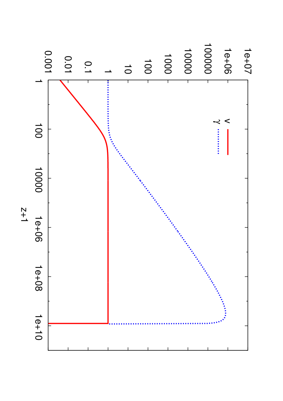
This equation of motion can be solved numerically assuming that the wall starts at rest at $T=T_{\rm C}=2\,{\rm MeV}$,³³ 3 We can show analytically that the velocity of the wall today depends only logarithmically on the initial temperature. and for $f=1$; the result is depicted in Fig. 2. We see that, right after its formation, the wall accelerates to a large boost factor, $\gamma\sim{\cal O}\left(10^{6}\right)$. However, it gradually slows down due to Hubble friction. The current peculiar velocity of the wall is $v_{0}\simeq 0.004$, so that none of the effects mentioned above is an issue. We also see that, in the non-relativistic regime, the velocity of the wall scales linearly with the parameter $f$.

To be viable, our model must satisfy an additional set of constraints that we now summarize.

1. 1.

   CMB constraints. While the effects of cosmic strings on the CMB have been extensively studied [38], domain walls have not been widely considered since they were thought to be formed at much higher energy and thus have a dramatic effect on the CMB.

   A single wall would contribute to the temperature anisotropy via the integrated Sachs Wolfe effect [39]. For a static universe, and in the non-relativistic regime, the gravitational potential generated by a very large (planar) wall grows linearly with the distance $L$ from the wall (notice that this has a zero net effect if the distance between the source and the wall is equal to that between the wall and the observer). For a typical cosmological distance $\sim H_{0}^{-1}$, we estimate $\delta T/T\sim G\,U_{\rm wall}\,H_{0}^{-1}$. This results in

   $$\left(\frac{\delta T}{T}\right)_{\rm CMB}\sim 10^{-6}\left(\frac{\eta}{1\,{\rm MeV}}\right)^{3}.$$

   (14)

   which constrains $\eta$ to be smaller than a few MeV. Another source of temperature anisotropy is related to the fact that $\alpha$ is not constant across the visible universe. This is not an issue for the model we are discussing, since the cmb data are only sensitive to a variation $\Delta\alpha/\alpha\sim{\cal O}\left(10^{-2}\right)$ or greater [40]. Finally, we can also neglect the temperature anisotropy related to the probability that a CMB photon is not transmitted through the wall, which is of ${\rm O}\left(\Delta\alpha/\alpha\right)^{2}$, as we have already mentioned.

2. 2.

   Astrophysical constraints. Although our scalar is relatively heavy, $m_{\phi}\sim 1$ MeV, it can be produced in supernovae. The production rate of scalars through inverse decay is roughly,

   $$\Gamma_{\gamma\gamma\to\phi}\sim\frac{\xi_{F}^{2}}{M_{*}^{2}}\,T^{3}.$$

   (15)

   In principle for scalars with mass $m_{\phi}<T$, this could result in an excessive energy loss rate. However, these scalars decay to two photons with a rate $\Gamma_{d}\sim\xi_{F}^{2}\mu^{3}/M_{*}^{2}\sim\xi_{F}^{2}M_{*}$. Requiring that their decay length is smaller than the size of the core leads to a lower bound on their mass

   $$\frac{M_{*}}{1\,{\rm MeV}}>\mathcal{O}(10^{-2})\times\left(\frac{10^{-6}}{\xi_{F}}\right)$$

   (16)

   (for typical energies of order $T\sim 30$ MeV). Thus, for our choice (9-10) of parameters, these scalars decay within the core and there is no energy loss.

3. 3.

   Tunnelling to the true vacuum. Contrary to a standard domain wall, the non-minimal coupling induces a shift between the two minima. The lifetime of the false vacuum is of the order [41]

   $$\tau\sim\Lambda\exp\left(\frac{27\pi^{2}}{8}\frac{S_{0}^{4}}{\Delta V^{3}}\right)$$

   with $S_{0}=\int_{-\eta}^{\eta}\sqrt{V(\phi)}{\rm d}\phi\sim 2\eta\sqrt{\Delta V}$. Now, with $\Delta V\sim\xi_{N}\Omega_{m0}\rho_{\rm crit}(\eta/M_{*})(1+z)^{3}$ and assuming $\Lambda\sim M_{*}^{-1}$, we conclude that $\tau=H_{0}^{-1}f_{\tau}$ with

   $$f_{\tau}=\frac{H_{0}}{M_{*}}\exp\left(\frac{54\pi^{2}}{\Omega_{m0}\xi_{N}}\frac{M^{4}_{*}}{\rho_{\rm crit}}\hat{\eta}^{3}(1+z)^{-3}\right).$$

   The argument in the exponential is always very large and scales as $4.5\times 10^{54}\hat{\eta}^{3}(1+z)^{-3}$. Even at the time the wall is formed, $z_{\rm f}\sim 10^{10}$, the factor is larger than $10^{24}$. This means that the wall forms at a time where the false vacuum has a lifetime larger than our Hubble time. Since the lifetime of the wall increases with time, we are guaranteed that today, the wall is effectively stable.

Our model also has some specific observational predictions that arise from the fact that $\alpha$ takes two discrete values. Let us denote ${\bf n}_{*}$ the direction of the wall and $z_{*}$ the redshift of its closest position and $\chi_{*}=\chi(z_{*})$ the comoving radial distance to which it corresponds. Since the equation of our past-light cone is $\chi=\eta_{0}-\eta$ and that of the wall $\chi=\chi_{*}/\cos\theta$ if it is assumed to be at rest in the cosmological rest frame. It follows that the redshift of the wall in a direction ${\bf n}$ is given by $\chi(z)=\chi_{*}/\cos\theta$ with $\cos\theta={\bf n}_{*}\cdot{\bf n}$. Solving this equation gives the dependence of $\alpha$ with $z$ and $\theta$ and is plotted in Fig. 3. Moreover since our observable universe as a finite radius, the discontinuity can be observed only in a cone of angle $\theta_{l}$ around the direction ${\bf n}_{*}$ with

$\theta_{l}$ depends on $z_{*}$ and on the cosmological parameters. Typically, $\cos\theta_{l}\sim 0.345$ if $z_{*}\sim 1.8$.

In summary, we have proposed a two vacuum solution to produce a large scale spatial variation of the fine structure constant, which is not associated to a local time variation. In the model presented, the scalar field was coupled to electromagnetism and to nucleons through the photon contribution to the nucleon mass. It is of course quite plausible that this coupling extends to other gauge fields (and perhaps Yukawa couplings) as well. In that case, we should expect not only spatial variations in $\alpha$, but also coupled spatial variations in other quantities such as particle masses and $\Lambda_{\rm QCD}$ [13, 42].

For example, one might expect a variation in the proton-to-electron mass ratio, $\mu$. If due to coupled variations of fundamental constants, one typically expects that it is correlated to the variation of $\alpha$; $\Delta\mu/\mu\sim-50\Delta\alpha/\alpha$ [43]. Molecular hydrogen transitions in quasar absorption systems yield a limit $\Delta\mu/\mu=(-2.6\pm 3.0)\times 10^{-6}$ [44]. Searches for spatial variations in the proton to electron mass ratio in the Milky Way [19] produced a non-zero result of $\Delta\mu/\mu=(2.2\pm 0.4\pm 0.3)\times 10^{-8}$ and conservatively implies an upper limit of $3\times 10^{-8}$. Analogous searches for a spatial variation of $\alpha^{2}\mu$ yield an upper limit of $3.7\times 10^{-7}$ [45]. Taken together, these would imply an upper limit of $\Delta\alpha/\alpha<2\times 10^{-7}$. In the context of the model presented here, this limit would present no difficulty with the Keck/Hires observations indicating a variation in $\alpha$. The Milky Way being entirely in the $\alpha_{+}$ vacuum would show no variations in any of these quantities and these observations therefore could not constrain variations in the $\alpha_{-}$ vacuum.

We also note that we might expect a small effect on the light element abundances produced in big bang nucleosynthesis [46]. Whether or not the transition happened before or after BBN, the average light element abundance should correspond to abundances using constants determined at $\phi=0$ (or at a slightly smaller value of $\alpha$). However variations at the level of $10^{-6}$ would hardly be perceptible in element abundances. Similarly a small change in $\alpha$ would very slightly affect the CMB through recombination [40], but this too would be imperceptible. The same may be true for future constraints that can be set from signals originating from the absorption of the CMB at 21 cm hyperfine transition of the neutral atomic hydrogen [47] or from stellar evolution [48] with sensitivities which are typically of the order of $10^{-2}$ for $z>30$ and $10^{-5}$ for $z\sim 15-20$ respectively.

Other standard powerful systems [1] for testing the variation in $\alpha$ are the Oklo phenomenon and meteoritic studies. But as these are both on our side of the wall, we would expect that they are too local to probe any variation in $\alpha$. Similarly, we would not expect any positive result from atomic clock measurements of changes in $\alpha$ unless of course the wall passes through the solar system in the near future. Given the sensitivity of these experiments (see e.g., Ref. [49]), there would be no mistaking the event.

References

- [1] J.-P. Uzan, Rev. Mod. Phys. 75, 403 (2003), [arXiv:hep-ph/0205340]; J.-P. Uzan, arXiv:1009.5514 [astro-ph.CO].
- [2] J.-P. Uzan, Gen. Rel. Grav. 42, 2219 (2010) [arXiv:0908.2243 [astro-ph.CO]]; J.-P. Uzan, Gen. Rel. Grav. 39, 307 (2007) [arXiv:astro-ph/0605313].
- [3] J. K. Webb, et al., Phys. Rev. Lett. 82 (1999) 884 [arXiv:astro-ph/9803165]; M. T. Murphy et al., Mon. Not. Roy. Astron. Soc. 327 (2001) 1208 [arXiv:astro-ph/0012419]; J. K. Webb et al., Phys. Rev. Lett. 87, 091301 (2001) [arXiv:astro-ph/0012539]; M. T. Murphy, et al., Mon. Not. Roy. Astron. Soc. 327 (2001) 1223 [arXiv:astro-ph/0012420]; M. T. Murphy, et al., Mon. Not. Roy. Astron. Soc. 345, 609 (2003) [arXiv:astro-ph/0306483].
- [4] G. R. Dvali and M. Zaldarriaga, Phys. Rev. Lett. 88, 091303 (2002) [arXiv:hep-ph/0108217]; T. Chiba and K. Kohri, Prog. Theor. Phys. 107 (2002) 631 [arXiv:hep-ph/0111086]; C. Wetterich, JCAP 0310, 002 (2003); C. Wetterich, Phys. Lett. B 561, 10 (2003) [hep-ph/0301261]; C. Wetterich, [hep-ph/0302116]; L. Anchordoqui and H. Goldberg, Phys. Rev. D 68, 083513 (2003) [arXiv:hep-ph/0306084]; Y. Fujii, Phys. Lett. B 573, 39 (2003) [arXiv:astro-ph/0307263]; E. J. Copeland, N. J. Nunes and M. Pospelov, Phys. Rev. D 69, 023501 (2004) [arXiv:hep-ph/0307299]; M. Peloso and E. Poppitz, Phys. Rev. D 68 (2003) 125009 [arXiv:hep-ph/0307379]; J.-P. Uzan, Phys. Rev. D 59, 123510 (1999) [arXiv:gr-qc/9903004]. D. S. Lee, W. Lee and K. W. Ng, Int. J. Mod. Phys. D 14, 335 (2005) [arXiv:astro-ph/0309316]; W. L. Lee, K. W. Ng and D. S. Lee, Mod. Phys. Lett. A 19, 1089 (2004); N. J. Nunes and J. E. Lidsey, Phys. Rev. D 69, 123511 (2004) [arXiv:astro-ph/0310882]. M. Byrne and C. Kolda, [arXiv:hep-ph/0402075]; P. P. Avelino, C. J. A. Martins and J. C. R. Oliveira, Phys. Rev. D 70, 083506 (2004) [arXiv:astro-ph/0402379]. Y. Fujii and S. Mizuno, Int. J. Mod. Phys. D 14, 677 (2005) [arXiv:astro-ph/0404222]; S. Lee, K. A. Olive and M. Pospelov, Phys. Rev. D 70, 083503 (2004); M. Doran, JCAP 0504, 016 (2005) [arXiv:astro-ph/0411606]; V. Marra and F. Rosati, JCAP 0505, 011 (2005) [arXiv:astro-ph/0501515]; P. P. Avelino, et al., Phys. Rev. D 74 (2006) 083508 [arXiv:astro-ph/0605690]; T. Chiba, et al., Phys. Rev. D 75, 043516 (2007) [arXiv:hep-ph/0610027]; S. Lee, Mod. Phys. Lett. A 22, 2003 (2007) [arXiv:astro-ph/0702063]; T. Dent, JCAP 0701, 013 (2007); M. E. Mosquera, et al., arXiv:0707.0661 [astro-ph].
- [5] H. B. Sandvik, J. D. Barrow and J. Magueijo, Phys. Rev. Lett. 88, 031302 (2002) [arXiv:astro-ph/0107512]; J. D. Barrow, H. B. Sandvik and J. Magueijo, Phys. Rev. D 65, 063504 (2002) [arXiv:astro-ph/0109414]; J. D. Barrow, J. Magueijo and H. B. Sandvik, Phys. Lett. B 541, 201 (2002) [arXiv:astro-ph/0204357].
- [6] M. Livio and M. Stiavelli, Ap. J. Lett. 507 (1998) L13 [arXiv:astro-ph/9808291]; S. J. Landau and H. Vucetich, Astrophys. J. 570, 463 (2002) [arXiv:astro-ph/0005316].
- [7] K. A. Olive and M. Pospelov, Phys. Rev. D 65, 085044 (2002) [arXiv:hep-ph/0110377].
- [8] T. Damour and A. M. Polyakov, Nucl. Phys. B 423, 532 (1994) [arXiv:hep-th/9401069]; T. Damour, F. Piazza and G. Veneziano, Phys. Rev. D 66, 046007 (2002) [arXiv:hep-th/0205111]; T. Damour and J. F. Donoghue, Phys. Rev. D 82, 084033 (2010) [arXiv:1007.2792 [gr-qc]].
- [9] H. Chand, et al., Astron. Astrophys. 417, 853 (2004) [arXiv:astro-ph/0401094]; R. Srianand, et al., Phys. Rev. Lett. 92, 121302 (2004) [arXiv:astro-ph/0402177].
- [10] R. Quast, D. Reimers and S. A. Levshakov, Astron. Astrophys. 415, L7 (2004) [arXiv:astro-ph/0311280].
- [11] M. T. Murphy, J. K. Webb and V. V. Flambaum, Phys. Rev. Lett. 99, 239001 (2007) [arXiv:0708.3677 [astro-ph]]; R. Srianand, et al., Phys. Rev. Lett. 99, 239002 (2007).
- [12] J. Khoury and A. Weltman, Phys. Rev. Lett. 93, 171104 (2004) [arXiv:astro-ph/0309300]; K. Hinterbichler and J. Khoury, Phys. Rev. Lett. 104, 231301 (2010) [arXiv:1001.4525 [hep-th]].
- [13] J. R. Ellis, et al., Phys. Lett. B 228, 264 (1989).
- [14] K. A. Olive and M. Pospelov, Phys. Rev. D 77, 043524 (2008) [arXiv:0709.3825 [hep-ph]].
- [15] B. Li, D. F. Mota and J. D. Barrow, arXiv:1009.1396 [astro-ph.CO].
- [16] J.K. Webb, et al., [1008.3907 [astroph.CO]].
- [17] J.C. Berengut, et al., [1009.0591 [astro-ph.CO]].
- [18] J. C. Berengut and V. V. Flambaum, arXiv:1008.3957 [physics.atom-ph].
- [19] S.A. Levshakov, P. Molaro, and M.G. Kozlov, [0808.0583 [astro-ph]]; P. Molaro, S.A. Levshakov, and M.G. Kozlov, M.G., Nucl. Phys. Proc. Suppl. 194 287, (2009) [0907.1192 [astro-ph.CO]]; S. A. Levshakov, et al., arXiv:0911.3732 [astro-ph.CO].
- [20] T. Ashenfelter, G. J. Mathews and K. A. Olive, Phys. Rev. Lett. 92, 041102 (2004); T. P. Ashenfelter, G. J. Mathews and K. A. Olive, Astrophys. J. 615, 82 (2004); M. G. Kozlov, et al., Phys. Rev. A 70, 062108 (2004).
- [21] K. Sigurdson, A. Kurylov and M. Kamionkowski, Phys. Rev. D 68, 103509 (2003) [arXiv:astro-ph/0306372].
- [22] J. Goodman, Phys. Rev. D 52, 1821 (1995); J.-P. Uzan, C. Clarkson, and G.F.R. Ellis, Phys. Rev. Lett. 100, 191303, (2008); R.R. Caldwell and A. Stebbins, Phys. Rev. Lett. 100, 191302 (2008); P. Dunsby et al., JCAP 06, 017 (2010).
- [23] T. Damour, G. W. Gibbons and C. Gundlach, Phys. Rev. Lett. 64, 123 (1990).
- [24] A. Coc, et al., Phys. Rev. D 79, 103512 (2009) [arXiv:0811.1845 [astro-ph]].
- [25] J. Gasser and H. Leutwyler, Phys. Rept. 87 (1982) 77.
- [26] J.D. Bekenstein, Phys. Rev. D 25, 1527, (1982).
- [27] S.M. Carroll, Phys. Rev. Lett. 81, 3067, (1998).
- [28] P. Peter, and J.-P. Uzan, Primordial Cosmology (Oxford Univ. Press, 2009).
- [29] A. Vilenkin and E. P. S. Shellard, Cosmic strings and other topological defects (Cambridge University Press, 2000).
- [30] A. E. Everett, Phys. Rev. D 10 3161 (1974); Ya. B. ZelÕdovich et al., Sov. Phys. JETP 40 1 (1975).
- [31] R.A. Battye, M. Bucher, and D. Spergel, [astro-ph/9908047].
- [32] Z. Chacko, C. Grojean, M. Perelstein, Phys. Lett. B 565, 169 (2003), [hep-ph/0204142].
- [33] D. Stauffer and A. Aharony, Introduction to percolation theory (Taylor and Francis, 1994); D. Stauffer, Scaling theory of percolation clusters, Phys. Rep. 54 1 (1979).
- [34] J. C. R. Oliveira, C. J. A. Martins and P. P. Avelino, Phys. Rev. D 71, 083509 (2005) [arXiv:hep-ph/0410356].
- [35] C. Schimd, J.-P. Uzan and A. Riazuelo, Phys. Rev. D 71, 083512 (2005) [arXiv:astro-ph/0412120].
- [36] B. Carter, [gr-qc/0012036]; R. A. Battye and B. Carter, Phys. Lett. B 509, 331 (2001) [arXiv:hep-th/0101061]. B. Carter and J.-P. Uzan, Nucl. Phys. B 606, 45 (2001) [arXiv:gr-qc/0101010].
- [37] P. P. Avelino, C. J. A. Martins and L. Sousa, Phys. Rev. D 78, 043521 (2008) [arXiv:0805.4013 [astro-ph]].
- [38] A. A. Fraisse, et al., Phys. Rev. D 78, 043535 (2008) [arXiv:0708.1162 [astro-ph]]; R. Durrer, M. Kunz and A. Melchiorri, Phys. Rept. 364, 1 (2002) [arXiv:astro-ph/0110348].
- [39] Y. B. Zeldovich, I. Y. Kobzarev and L. B. Okun, Zh. Eksp. Teor. Fiz. 67, 3 (1974) [Sov. Phys. JETP 40, 1 (1974)].
- [40] G. Rocha, et al. Mon. Not. Roy. Astron. Soc. 352, 20 (2004) [arXiv:astro-ph/0309211]. M. Nakashima, R. Nagata and J. Yokoyama, Prog. Theor. Phys. 120, 1207 (2008) [arXiv:0810.1098 [astro-ph]]; E. Menegoni, et al., Phys. Rev. D 80, 087302 (2009) [arXiv:0909.3584 [astro-ph.CO]]; C. J. A. Martins, et al., Phys. Rev. D 82, 023532 (2010) [arXiv:1001.3418 [astro-ph.CO]]. S. J. Landau and C. G. Scoccola, arXiv:1002.1603 [astro-ph.CO].
- [41] S. Coleman, Aspects of symmetry (Cambridge Univ. Press, 1985).
- [42] B. A. Campbell and K. A. Olive, Phys. Lett. B 345, 429 (1995) [arXiv:hep-ph/9411272].
- [43] K. A. Olive, et al., Phys. Rev. D 66 (2002) 045022 [arXiv:hep-ph/0205269].
- [44] J. A. King, et al., Phys. Rev. Lett. 101, 251304 (2008) [arXiv:0807.4366 [astro-ph]].
- [45] S. A. Levshakov, P. Molaro and D. Reimers, arXiv:1004.0783 [astro-ph.CO].
- [46] V. F. Dmitriev, V. V. Flambaum and J. K. Webb, Phys. Rev. D 69, 063506 (2004) [arXiv:astro-ph/0310892]; A. Coc, et al., Phys. Rev. D 76, 023511 (2007) [arXiv:astro-ph/0610733]; J. C. Berengut, V. V. Flambaum and V. F. Dmitriev, Phys. Lett. B 683, 114 (2010) [arXiv:0907.2288 [nucl-th]].
- [47] R. Khatri and B. D. Wandelt, Phys. Rev. Lett. 98, 111301 (2007) [arXiv:astro-ph/0701752].
- [48] S. Ekstrom, et al., Astron. Astrophys. 514, A62 (2010). [arXiv:0911.2420 [astro-ph.SR]].
- [49] T. Rosenband, et al., Science 319, 1808 (2008).