Non-degenerate shell-model effective interactions from
the Okamoto-Suzuki and Krenciglowa-Kuo iteration methods
Abstract
We present calculations of shell-model effective interactions for both degenerate and non-degenerate model spaces using the Krenciglowa-Kuo (KK) and the extended Krenciglowa-Kuo iteration method recently developed by Okamoto, Suzuki et al. (EKKO). The starting point is the low-momentum nucleon-nucleon interaction obtained from the N3LO chiral two-nucleon interaction. The model spaces spanned by the and shells are both considered. With a solvable model, we show that both the KK and EKKO methods are convenient for deriving the effective interactions for non-degenerate model spaces. The EKKO method is especially desirable in this situation since the vertex function -box employed therein is well behaved while the corresponding vertex function -box employed in the Lee-Suzuki (LS) and KK methods may have singularities. The converged shell-model effective interactions given by the EKKO and KK methods are equivalent, although the former method is considerably more efficient. The degenerate -shell effective interactions given by the LS method are practically identical to those from the EKKO and KK methods. Results of the one-shell and two-shell calculations for 18O, 18F, 19O and 19F using the EKKO effective interactions are compared, and the importance of the shell-model three-nucleon forces is discussed.
pacs
21.60.Cs, 21.30.-x,21.10.-kI I. Introduction
The nuclear shell model has provided a very successful framework for describing the properties of a wide range of nuclei. This framework is basically an effective theory [1, 2, 3], corresponding to reducing the full-space nuclear many-body problem to a model-space one with effective Hamiltonian =, where is the single-particle (s.p.) Hamiltonian and represents the projection operator for the model space which is usually chosen to be a small shell-model space such as the shell outside of an closed core. The effective interaction plays a central role in this nuclear shell model approach, and its choice and/or determination have been extensively studied, see e.g. [4, 5, 2, 3]. As discussed in these references, may be determined using either an empirical approach where it is required to reproduce selected experimental data or a microscopic one where is derived from realistic nucleon-nucleon (NN) interactions using many-body methods. The folded-diagram theory [1, 2, 3] is a commonly used such method for the latter. Briefly speaking, in this theory is given as a folded-diagram series [1, 2, 3, 6]
| (1) |
where represents a so-called -box, which may be written as
| (2) |
Here represents the NN interaction and is the so-called starting energy which will be explained later (section II). Thus from the NN interaction we can in principle calculate the -box and thereby the effective interaction . Note that we use , without hat, to denote the -space projection operator. (.) Note also that the -box is an irreducible vertex function where the intermediate states between any two vertices must belong to the space. As indicated by the subscript in eq. (2), the -box contains valence linked diagrams only, such as the 1st- and 2nd-order -box diagrams for and shown in Fig. 1. The -box of eq. (1) is defined as (), namely begins with diagrams 2nd-order in . The above folded-diagram formalism has been employed in microscopic derivations of shell model effective interactions for a wide range of nuclei [2, 3].
In the present work we would like to explore an extension of the well-known methods for computing the folded diagram series in eq. (1). The Lee-Suzuki (LS) [7, 8, 9] iteration scheme has been commonly used in previous microscopic calculations of shell model effective interactions [2, 3]. Here we would like to employ two different methods, the Krenciglowa-Kuo (KK) iteration method [10, 11] and the newly developed extended Krenciglowa-Kuo iteration method of Okamoto, Suzuki, Kumagai and Fujii (EKKO)[12], mainly for the purpose of calculating the shell-model efective interactions for non-degenerate model spaces. As we shall discuss later, it is not convenient to use the LS method for calculating the effective interactions for non-degenerate model spaces such as the two-shell case, while both the EKKO and the KK methods can be conveniently applied in this situation. The EKKO method has an additional advantage. When the - and -space are not adequately separated from each other, the -box employed in the KK method may have singularities, causing difficulty for its iterative solution. An essential and interesting difference between the EKKO and KK methods is that the EKKO method employs the vertex function -box (to be defined in section II) while in the latter the vertex function -box is used. This simple replacement (of by ) has an important advantage in circumventing the singularities mentioned above. As we shall discuss later, both the EKKO and KK methods may provide a suitable framework for calculating shell-model effective interactions for large non-degenerate model spaces which may be needed for describing exotic nuclei with large neutron excess.
The organization of the present paper is as follows. In section II we shall describe a non-degenerate version of the EKKO method [12] and how we apply it and the KK method [10, 11] to shell-model effective interactions. A comparison of these two methods with the LS scheme [7, 8] will be made. Our results will be presented and discussed in section III. We shall first perform a sequence of model calculations comparing the EKKO, KK and LS iteration methods for both degenerate and non-degenerate model spaces. The use of the EKKO and KK methods in calculating the effective interactions for non-degenerate model spaces will be emphasized. Starting from the interaction [14, 15, 16, 3] derived from the chiral N3LO potential [17], the LS, KK and EKKO methods will all be used to calculate the degenerate one-shell effective interactions, a main purpose being to check if the results given by the commonly used LS method agree with the KK and EKKO ones. The KK and EKKO methods will then be employed to calcualte the non-degenerate two-shell effective interactions. The matrix elements of the above degenerate and non-degenerate interactions will be compared. The low-energy spectra of 18O, 18F, 19O and 19F given by these interactions will be discussed. A summary and conclusion will be presented in section IV.

II II. Formalism
In this section, we shall describe and discuss the KK [10, 11] and the EKKO [12] iteration methods and their application to microscopic calculations of shell-model effective interactions. These methods, to our knowledge, have not yet been employed in such calculations. Let us begin with a brief review of the LS [7, 8] and KK iteration methods. Consider first the degenerate LS method where the model space is degenerate, namely , being a constant. In terms of the -box of Eq.(2), the effective interactions are calculated iteratively by [7, 8]
| (3) |
| (4) |
and for
| (5) |
where is proportional to the derivative of :
| (6) |
The effective interaction is given by the converged , namely
| (7) |
There is a practical difficulty for the above iteration method. In actual shell-model calculations, it is usually not possible to calculate the vertex function -box exactly; thus it is a common practice to evaluate it with some low-order approximation and calculate the derivatives numerically. At higher orders this becomes increasingly difficult, and therefore such calculations are usually limited to low orders in the iteration. However, as we shall demonstrate in section IIIa, low-order LS iterations are often not accurate when the - and -spaces are strongly coupled.
The above degenerate LS iteration method can be generalized to a non-degenrate one [9], namely being non-degenerate. In this situation we need not only the -box of eq. (2) but also a generalized -box defined by
| (8) |
with
| (9) |
This generalized -box is defined for , and is defined by where . The dimension of the -space is labelled . Note that only valence-linked diagrams are retained in , as indicated by the subscript L.
With the above definitions, the effective interaction given by the non-degenerate LS iteration method is given as [9]
| (10) | |||||
with , . In the above equations . When convergent, we have . The above non-degenerate LS method can be used to calculate the effective interactions for e.g., the non-degenerate -shell [13] or the two-shell model space. But this method is rather complicated for computations, and this has hindered its application to microscopic calculations of shell-model effective interactions.
We now describe some details of the non-degenerate KK and EKKO methods. The KK iteration method was originally developed for model spaces which are degenerate [10]. A non-degenerate KK iteration method was later formulated [11], with the effective interaction given by the following iteration methods. Let the effective interaction for the ith iteration be and the corresponding eigenvalues and eigenfunctions be given by
| (11) |
Here is the -space projection of the full-space eigenfunction , namely . The effective interaction for the next iteration is then
| (12) |
where the bi-orthogonal states are defined by
| (13) |
Note that in the above is non-degenerate. The converged eigenvalue and eigenfunction satisfy the -space self-consistent condition
| (14) |
To start the iteration, we use
| (15) |
where is a starting energy chosen to be close to . The converged KK effective interaction is given by . When convergent, the resultant is independent of , as it is the states with maximum -space overlaps which are selected by the KK method [10]. We shall discuss this feature later in section III using a solvable model. The above non-degenerate KK method is numerically more convenient than the non-degenerate LS method.
The diagrams of Fig. 1 have both one-body (d1,d2,d3) and two-body (d4,d5,d6,d7) diagrams. When we calculate nuclei with two valence nucleons such as and , all seven diagrams are included in the -box. But for nuclei with one valence nucleon such as , we deal with the 1-body -box which is approximated by the sum of diagrams d1, d2 and d3. The 1-body effective interaction is given by a similar KK iteration
| (16) |
Denoting its converged value as , the model-space s.p. energy is given by . By adding and then subtracting , we can rewrite Eq.(14) as
| (17) |
with . In most shell model calculations [4, 5], one often uses the experimental s.p. energies. This treatment for the s.p. energies is in line with the above subtraction procedure, as represents the physical s.p. energy which in principle can be extracted from experiments. In the present work we shall use the experimental s.p. energies for the model-space orbits together with the derived from (). A similar subtraction procedure has also been employed in the LS calculations [2, 3] where the all-order sum of the one-body diagrams was subtracted from the calculation of the effective interaction.
In several aspects, the above KK method provides a more desirable framework for effective interaction calculations than the commonly used LS method. The KK method is more convenient for non-degenerate model spaces than the LS method, and the KK method does not require the calculation of high-order derivatives of the -box, which may be necessary in a converged LS calculation. The KK method has, however, a shortcoming when applied to calculations with extended model space such as the two-shell one. For example, certain 2nd-order diagrams for this case may diverge, resulting in an ill-defined -box. It is remarkable that these potential divergences can be circumvented by the recently proposed EKKO method of Okamoto et al. [12]. In this method, the vertex function -box is employed. It is related to the -box by
| (18) |
where is the first-order derivative of the -box. The -box considered by Okamoto et al. [12] is for degenerate model spaces (), while we consider here a more general case with non-degenerate . An important property of the above -box is that it is finite when the -box is singular (has poles). Note that satisfies
| (19) |
The iteration method for determining the effective interaction from the -box is quite similar to that for the -box. Suppose the effective interaction for the th iteration is . The corresponding eigenfunction and eigenvalues are determined by
| (20) |
The effective interaction for the next iteration is
| (21) |
Although and are generally different, it is interesting that the converged eigenvalues of and the corresponding ones of are both exact eigenvalues of the full-space Hamiltonian , which can be seen from eqs. (14), (18) and (19). Note, however, the KK and EKKO methods may reproduce different eigenvalues of the full-space Hamiltonian . This aspect together with some other comparisons of these methods will be discussed in section IIIa, using a simple solvable model.
For the degenerate case, Okamoto et al. [12] have shown that =0 at the self-consistent point . As outlined below, we have found that this result also holds for the case of non-degenerate . From eq. (18), we have
| (22) | |||||
Then from eqs. (14) and (19) we have
| (23) |
and
| (24) |
This is a useful result; it states that at any self-consistent point the eigenvalues varies ‘flatly’ with , a feature certainly helpful to iterative calculations. In section III, we shall check this feature numerically.
III III. Results and discussion
III.1 IIIa. Model calculations comparing the LS, KK and EKKO methods
In this section we shall study the above iteration methods by way of a simple matrix model, similar to the one employed in [12]. We consider a 4-dimensional matrix Hamiltonian where
| (25) |
and
| (26) |
The interaction Hamiltonian has a strength parameter , namely
| (27) |
with
As discussed in section II, both the KK and EKKO iteration methods are rather convenient for non-degenerate model spaces. We would like to check this feature by carrying out some calculations using the above model. We consider two unperturbed Hamiltonians, given by =(0,6,4,9) and (0,0,4,9). The parts of them are, respectively, non-degenerate and degenerate.
In the first three entries of Table I, some results for the =(0,6) case are presented. Here are the exact eigenvalues of the full Hamiltonian, with their model-space overlaps denoted by . The entries and are the eigenvalues generated respectively by the KK and EKKO iteration methods. Not only is the above non-degenerate but its spectrum intersects that of . One would expect that this may cause difficulty for the above iteration methods. But as indicated in Table I, both the non-degenerate KK and the non-degenerate EKKO iteration methods work remarkably well. Note that the interaction used here is rather strong (x=0.6), and both methods still work well, converging to values of which are quite far from .
Some results for the degenerate case of =(0,0) are listed in the last two entries of Table I. Here we have performed calculations using the degenerate LS method through 5th order iteration (i.e. in Eq.(7) we use ). As shown, the results so obtained are not in good agreement with the exact results. This suggests that low-order LS iteration method may often be inadequate, and one needs higher-order iterations to obtain accurate results.
It is known that the KK iteration method converges to the states with maximum -space overlaps [10], while the LS method converges to the states of lowest energies [7, 8]. We have found that for many cases the EKKO method also converges to states of maximum -space overlaps. As listed in the third entry of Table I, both the KK and EKKO methods converge to states of energies = -3.51 and 14.53 whose -space probabilities are relatively 0.70 and 0.86. We have also found that the EKKO and KK iteration methods can converge to different states. An example is the result shown in the last part of Table I, where the EKKO method converges to states of energy (-space probability) -1.45 (0.87) and 0.91 (0.46), while the states of maximum -space overlap are those with energies -1.45 and 5.25. Note that for this case the EKKO method is clearly more accurate than the KK method.
We have noticed that for a number of cases the EKKO method converges well but not so for the KK method. This is largely because these two methods treat the singularities of the -box differently. To see this, let us perform a graphical solution for the x=0.60 case of Table I. Using the parameters of this case, we calculate and plot in Fig. 3 both and which are respectively the eigenvalues of and . As discussed in section II, they have identical self-consistent solutions, namely where is the eigenvalue of the full-space Hamiltonian. Recall that and are given respectively by eqs. (2) and (18). As shown in the figure, the curves of and do have identical self-consistent solutions as marked by the common intersection points , , and . Note that the above two curves are distinctly different from each other, particularly in the vicinity of the poles (marked by the vertical lines through and ) of the -box. There is discontinuous, diverging oppositely before and after the pole, while remains continuous throughout. This clearly helps the convergence of the -box iteration method: The -box iteration proceeds along a continuous curve, while the -box iteration often does not converge as it may bounce back and forth across the discontinuity.
As seen from eq. (18), the -box method has ‘false’ solutions at , where are poles of the -box. These solutions are marked in Fig. 3 as and . These false solutions can be readily recognized and discarded. As given in Eq.(24), we have at self-consistent points . As shown in Fig. 3, the slopes of do satisfy the above condition at the self-consistent points to , but not so at the false points and .
| = (0,6,4,9) | x=0.10 | |||
|---|---|---|---|---|
| -0.110705 | 3.328164 | 7.203243 | 8.579299 | |
| 0.991108 | 0.044558 | 0.953368 | 0.010966 | |
| -0.110705 | 7.203243 | |||
| -0.110705 | 7.203242 | |||
| x =0.30 | ||||
| -0.974184 | 1.808716 | 8.080888 | 10.084581 | |
| 0.906155 | 0.111257 | 0.113523 | 0.869066 | |
| -0.974185 | 10.084580 | |||
| -0.974185 | 10.084581 | |||
| x =0.60 | ||||
| -3.510377 | -0.286183 | 8.265089 | 14.531471 | |
| 0.709531 | 0.189318 | 0.232422 | 0.868729 | |
| -3.510377 | 14.531472 | |||
| -3.510363 | 14.531472 | |||
| =(0,0,4,9) | x= 0.10 | |||
| -0.296201 | 0.982861 | 3.736229 | 8.577111 | |
| 0.985416 | 0.922993 | 0.082811 | 0.008780 | |
| -0.314591 | 0.872176 | |||
| -0.296201 | 0.982860 | |||
| -0.296201 | 0.982860 | |||
| x= 0.30 | ||||
| -1.448782 | 0.906504 | 5.254129 | 8.288149 | |
| 0.868986 | 0.460296 | 0.566014 | 0.104704 | |
| -1.620734 | 0.339561 | |||
| -1.125579 | 5.515468 | |||
| -1.448782 | 0.906504 |

III.2 IIIb. The and shell model effective interactions
In this subsection, we shall calculate the effective interactions for both the degenerate one-shell and the non-degenerate two-shell cases. Before presenting our results, let us first describe some details of our calculations. The LS, KK and EKKO methods as described in section II will be employed. We first compute the low-momentum nucleon-nucleon interaction [14, 15, 16, 3] starting from the chiral N3LO two-body potential [17] at a decimation scale of 2.1 fm-1. At this cutoff scale, the low-momentum interactions derived from different NN potentials [17, 18, 19, 20] are remarkably close to each other, leading to a nearly unique low-momentum interacton [16]. The effect of the leading-order chiral three-nucleon force on shell model effective interactions has been studied, and our results will be reported in a separate publication [21]. The above interaction is then used in calculating the -box diagrams as shown in Fig. 1. In calculating these diagrams, the hole orbits are summed over the shells and particle orbits over the shells. The active spaces (-space) used for the one-shell and two-shell calculations are respectively the three orbits in the shell and the seven orbits in the shells. The experimental s.p. energies of (0.0, 5.08, 0.87) MeV have been used, respectively, for the () orbits [22]. We have employed the shell-model s.p. wave functions and energies with the harmonic oscillator constant of =14 MeV.


In the following, let us first report our results for the degenerate one-shell calculations. Here by degenerate we mean that the unperturbed s.p. energy levels for the () orbits are degenerate. Our purpose here is mainly to compare the results given by the KK and EKKO method with those given by the commonly used degenerate LS method [2, 3]. Our results are presented in Figs. 3 and 4. As discussed in section II and illustrated in Table I, the EKKO and KK methods may converge to different states. In the present calculations they actually converge to the same states, as seen in Figs. 3 and 4. Our LS calculations are carried out using a low-order approximation, namely we take (see eq. (7)). As shown in the figures, the LS, KK and EKKO results for both 18O and 18F are in fact nearly identical to each other. A comparison of our results with experiments [22] is also presented in the figures. The agreement between our calculated energy levels with experiments is moderately satisfactory for 18O, but for 18F the calculated lowest states, though of correct ordering, are all significantly higher than the experimental values. As discussed in sections II and IIIa, the LS method is known to converge to the states of the lowest energies, while the KK method to the states of maximum -space overlaps. Thus the good agreement shown in Figs. 3 and 4 is an important indication that the states reproduced by the model-space LS, EKKO and KK effective interaction are likely those of the lowest energies as well as maximum model-space overlaps. In Fig. 5, we compare the entire -shell matrix elements given by the LS and EKKO methods; it is remarkable that every individual LS matrix element is practically equal to the corresponding EKKO one. (The matrix elements given by EKKO and KK are also nearly identical.) Recall that our LS matrix elements were obtained with a low-order iteration, which indicates the rapid convergence of the iteration scheme in the case of -shell effective interactions.
As discussed in sections II and IIIa, the EKKO or KK methods are convenient for deriving the effective interactions for non-degenerate model spaces. In the following let us first apply these methods to a relatively simple case, namely the non-degenerate one-shell effective interactions. The shell-model s.p. energies for the shell are degenerate, but the experimental ones are not. It may be of interest to employ the experimental s.p. energies as the unperturbed s.p. energies for the shell [3]. Thus here we employ the same unperturbed s.p. spectrum as the previous degenerate case except that the and orbits are shifted upward by, respectively, 5.08 and 0.87 MeV relative to the , mimicking the experimental s.p. energies. We have found that the non-degenerate and degenerate EKKO effective interactions do not differ significantly from each other. To illustrate, we compare in Fig. 6 the spectra of 19F for both the degenerate and non-degenerate -shell calculations; they agree with each other rather well. Slightly better agreements between the spectra of , and calculated with these two interactions are also observed. In short, the one-shell effective interactions given by the degenerate and non-degenerate choices for the unperturbed s.p. energies are nearly the same, and it is adequate in this case to just use the former choice.


We now report our results for the non-degenerate two-shell effective interactions. So far our calculations have all been carried out using the one-shell model space. For certain nuclei such as those with a large neutron excess, a larger model space such as the one may be needed. It will be convenient to describe our calculations by way of an example, namely 18O. Consider the states of this nucleus. In the one-shell case, the model space is spanned by three basis states , where , or . For the case, the model space is enlarged, having four additional single-particle states labeled by ). The whole model space is now non-degenerate as the orbits are one shell above the ones. Similar to the one-shell case, we have calculated the effective interactions using both the EKKO and KK methods. For the shell-model calculations, we have employed the experimental s.p. energies for the three -shell orbits as mentioned earlier.
For the shell-model calculations, we need in addition the experimental s.p. energies for the four orbits. Their values are, however, not well known. In the present calculation we have placed them all at a separation of one (14 MeV) above the level. (As to be reported later (Fig. 11), we shall also use a smaller value for the above separation.) In our calculations we have considered two choices for the unperturbed s.p. energies of the model space, a degenerate one and a non-degenerate one (in which the and orbits are shifted higher in energy compared to the orbit as described earlier). We have found that the results are rather similar, and in the following discussion we report only the calculations for the degenerate -shell choice.
In Fig. 7 we compare the matrix elements of the two-shell EKKO interaction with those of the one-shell case. Only the matrix elements within the shell are shown. We find that the magnitudes of the two-shell matrix elements are generally weaker than the one-shell matrix elements, some differing by as much as 1 MeV. Despite these differences, the resulting spectra for 18O and 18F given by the one-shell and two-shell calculations are nearly equivalent to each other, as illustrated by the two middle columns of Fig. 8. In our present and subsequent calculations we employ a low-order -box consisting of the 1st- and 2nd-order diagrams of Fig. 1. It is instructive, however, to compare the one- and two-shell calculations when only the leading-order approximation to the -box is retained. In the two leftmost columns of Fig. 8 we show the spectra of 18F when only the 1st-order -box diagrams are included. We note that in this case (in contrast to the second-order -box calculation) the resulting ‘1 Shell’ and ‘2 Shell’ spectra are largely different.
This important observation can be explained as follows. In general, the different and model spaces will result in different effective interactions and associated effective Hamiltonians, which we denote by and . But since the model space is a subspace of model space, and should in principle have common eigenvalues. We would like to check that this requirement is satisfied by our present calculations. As indicated by the two middle columns of Fig. 8, we see that indeed this is the case. In fact among the many states given by the calculations, it is the ones with the maximum -space overlaps which agree with the results given by the -shell calculation, which is a physically desirable result. Because of the difference in the model spaces, the renormalization effects for the and effective interactions are different. To bridge these differences, we need to include at least the 2nd-order -box diagrams (note that the allowed intermediate states of the 2nd-order -box diagrams are model-space dependent). These diagrams are not included in the above 1st-order calculations, and consequently the and results are different as shown by the two leftmost columns of Fig. 8, which is a strong evidence for the importance of the model-space-dependent renormalization effects. The construction of model-space effective interactions is in many ways similar to the construction of an effective theory from a renormalization group evolution. In such cases, one would expect that despite the different effective Hamiltonians, the same low-energy physical observables would be reproduced. The shell model effective interactions in the present work have not been computed exactly (that is, including high-order diagrams in the -box), yet it is interesting that we nevertheless find excellent agreement between the one- and two-shell calculations including -box diagrams only up to second order.


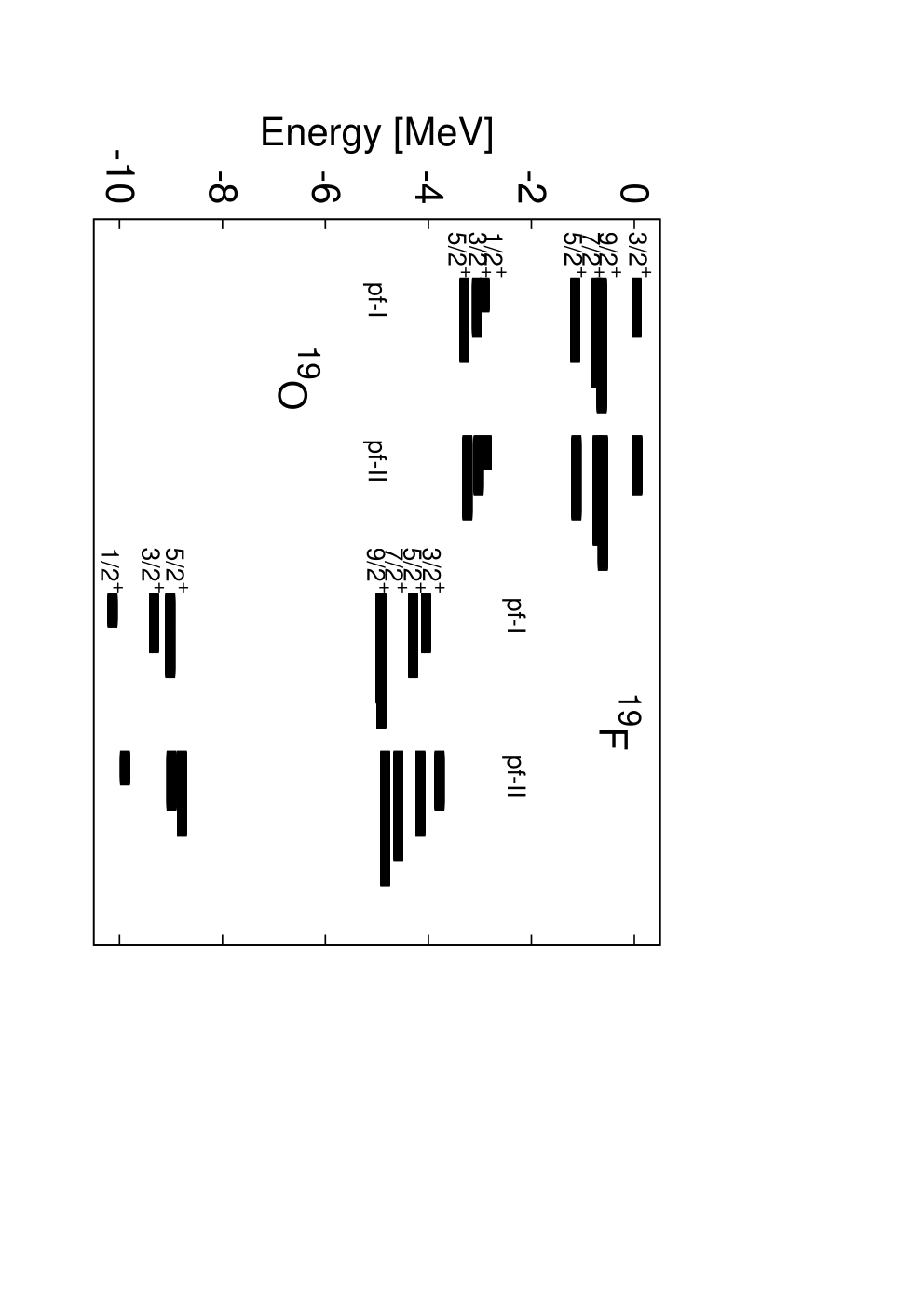

To further study the one-shell and two-shell effective interactions, we have applied them to shell model calculations of 19O and 19F. The 2nd-order -box of Fig. 1 is employed. Our results are displayed respectively in Figs. 9 and 10. It is of interest that the one-shell and two-shell results for 19O are nearly identical, and for 19F they are also remarkably close to each other. Although the orderings of our calculated spectra are in fair agreements with experiments, there are significant differences between them. As discussed earlier, in our two-shell calcualtions the experimental s.p. energies for the four orbits are needed, but their values are not well known. So far we have chosen to place them at a separation of 14 MeV above the orbit. We have repeated our calculations using instead a smaller separation of 10 MeV, to investigate if the use a smaller separation may improve the agreements. As illustrated in Fig. 11, the low-lying states of are hardly changed, those given by the separations of 14 and 10 MeV being nearly identical. The differences between the two sets of states for are also generally small. That these low-lying states are insensitive to the above separations indicates that our effective interactions (obtained with the inclusion of the 1st- and 2nd-order -box diagrams of Fig. 1) have a rather weak coupling between the and shells.
Recall that we have employed the folded-diagram expansion of eq. (1) to calculate the effective interaction . For nuclei with three valence nucleons, this expansion has both 2-body and 3-body diagrams. (By 3-body diagrams we mean those valence-linked diagrams with three incoming and three outgoing valence lines [1].) As an example, the shell-model three-nucleon force diagram of Fig. 12 should be included in the one-shell effective interaction for 19O and 19F. But this diagram is not included in our present one-shell calculation as we employ only the two-body -box of Fig. 1. This diagram is, however, included in our shell model calculations for 19O and 19F. Thus the good agreement between the one-shell and two-shell results shown in Fig. 9 is an indication that this type of shell-model three-nucleon force is likely to have little importance for 19O spectra, while it is moderately important for 19F as suggested by the small difference shown in Fig. 10. Further studies of this type of three-nucleon force will be useful and of interest, and we plan to do so in a future study.
IV IV. Summary and conclusion
We have applied the iteration method of Krenciglowa and Kuo (KK) and that recently developed by Okamoto et al. (EKKO) to the microscopic derivation of the and shell-model effective interactions using the low-momentum nucleon-nucleon interaction derived from the chiral two-body potential. We first considered a solvable model and found that both methods are suitable and efficient for deriving the effective interactions for non-degenerate model spaces, where the Lee-Suzuki iteration method is considerably less convenient. Even in the situation where the - and -space unperturbed Hamiltonians have spectrum overlaps did the KK and EKKO methods perform remarkably well. The EKKO method has the special advantage that its vertex function -box is, by construction, a continuous function of the energy, while the -box function used in the LS and KK methods may have singularities. This feature was found to be particularly useful for the convergence of the EKKO iteration method.
Using the low-momentum potentialss obtained from above two-body interaction, we first calculated the degenerate one-shell effective interactions using the LS, KK and EKKO methods. The results given by KK and EKKO were found to be identical. It is noteworthy that the LS results, calculated with a low-order (5th order) iteration, were also in very good agreement with both the KK and EKKO results, supporting the accuracy of the low-order LS method for calculating the degenerate shell-model effective interactions.
We have calculated the non-degenerate two-shell effective interactions using both the EKKO and KK methods. Both methods gave identical results and were found to be suitable for such non-degenerate calculations, with the former being more efficient (faster converging). We have applied these interactions to compute the low-lying energy spectra for several nuclei with two and three valence nucleons above the 16O core. Since the model space is a subspace of the model space, we expect the effective Hamiltonians for these two spaces to have common eigenvalues. Indeed this was largely confirmed in our calculations of 18O, 18F, 19O and 19F spectra, where it was found that the states in the calculations with the maximum -space overlap agreed with the results given by the calculations. The above agreement was found to be excellent for 19O, though not as good for 19F, which indicates that the shell-model three-nucleon force is more important in 19F (where the proton-neutron interaction is involved) than in 19O. Further study of this three-nucleon force should be useful and of much interest.
The calculated ground state energies for the above four nuclei are all higher (less bound) than the corresponding experimental values. We are studying if the inclusion of the chiral three-nucleon force may give additional binding energy [21]. In the present work we have employed the -box irreducible vertex function consisting of the first- and second-order diagrams only. The inclusion of the Kirson-Babu-Brown (KBB) all-order core polarization diagrams in the -box may provide additional binding energy [23]. We plan to carry out futher calculations with the inclusion of such all-order KBB diagrams.
Acknowledgements.
We are very grateful to L. Coraggio, A. Covello, A. Gargano, Jason Holt, N. Itaco, M. Machleidt, R. Okamoto and K. Suzuki for many helpful discussions. Partial supports from the US Department of Energy under contracts DE-FG02-88ER40388 and the DFG (Deutsche Forschungsgemeinschaft) cluster of excellence: Origin and Structure of the Universe are gratefully acknowledged.References
- [1] T. T. S. Kuo and E. Osnes, Lecture Notes in Physics (Springer-Verlag, New York, 1990), Vol. 364.
- [2] M. Hjorth-Jensen, T. T. S. Kuo, and E. Osnes, Phys. Rep. 261, 126 (1995), and references therein.
- [3] L. Coraggio, A. Covello, A. Gargano, N. Itaco and T.T.S. Kuo, Prog. Part. Nucl. Phys., 62 (2009) 135, and references quoted therein.
- [4] B.A. Brown and B.H. Wildenthal, Ann. Rev. Nucl. Part. Sci. 38, 29(1988).
- [5] B.A. Brown, W.A. Richter, Phys. Rev. C74, 0343150 (2006).
- [6] T.T.S. Kuo, S.Y. Lee and K.F. Ratcliff, Nucl. Phys. A176 (1971) 172.
- [7] S.Y. Lee and K. Suzuki, Phys. lett. 91B, 173 (1980).
- [8] K. Suzuki and S.Y. Lee, Prog. Theor. Phys. 64, 2091 (1980).
- [9] K. Suzuki, R. Okamoto, P.J. Ellis and T.T.S. Kuo, Nucl. Phys. A567 (1994) 576.
- [10] E.M. Krenciglowa and T.T.S. Kuo, Nucl. Phys. A235, 171 (1974).
- [11] T.T.S. Kuo, F. Krmpotic, K. Suzuki and R. Okamoto, Nucl. Phys. A582, 205(1995).
- [12] R. Okamoto, K. Suzuki, H. Kumagai and S. Fujii, to be published in ‘Proceedings of the 10th International Spring Seminar on Nuclear Physics (May 21-25, Sur Mare Vietri, Italy, ed. by A. Covello)’; [nucl-th] arXiv:1011.1994v1.
- [13] L. Coraggio and N. Itaco, Phys. Lett. B616, 43 (2005).
- [14] S. K. Bogner, T. T. S. Kuo and L. Coraggio, Nucl. Phys. A684, (2001) 432.
- [15] S.K. Bogner, T.T.S. Kuo, L. Coraggio A. Covello, and N. Itaco, Phys. Rev. C 65, 051301(R) (2002).
- [16] S. K. Bogner, T. T. S. Kuo, and A. Schwenk, Phys. Rep. 386, 1 (2003).
- [17] D. R. Entem, R. Machleidt, and H. Witala, Phys. Rev. C 65, 064005 (2002).
- [18] R. Machleidt, Phys. Rev. C 63, 024001 (2001).
- [19] R. B. Wiringa, V. G. J. Stoks, and R. Schiavilla, Phys. Rev. C 51, 38 (1995).
- [20] V. G. J. Stoks, R. A. M. Klomp, C. P. F. Terheggen, and J. J. de Swart, Phys. Rev. C 49, 2950 (1994).
- [21] H. Dong, T.T.S. Kuo and J. W. Holt, preprint (May 2011, to be submitted to arXiv and PRC).
- [22] http://www.nndc.bnl.gov/chart/.
- [23] J.D. Holt, J. W. Holt, T. T. S. Kuo, G. E. Brown and S. K. Bogner, Phys. Rev. C72, 041304(R) (2005).