Commensurability effects in one-dimensional Anderson localization: anomalies in eigenfunction statistics
Abstract
The one-dimensional (1d) Anderson model (AM), i.e. a tight-binding chain with random uncorrelated on-site energies, has statistical anomalies at any rational point , where is the lattice constant and is the de Broglie wavelength. We develop a regular approach to anomalous statistics of normalized eigenfunctions at such commensurability points. The approach is based on an exact integral transfer-matrix equation for a generating function ( and have a meaning of the squared amplitude and phase of eigenfunctions, is the position of the observation point). This generating function can be used to compute local statistics of eigenfunctions of 1d AM at any disorder and to address the problem of higher-order anomalies at with . The descender of the generating function is shown to be the distribution function of phase which determines the Lyapunov exponent and the local density of states.
In the leading order in the small disorder we have derived a second-order partial differential equation for the -independent (”zero-mode”) component at the () anomaly. This equation is nonseparable in variables and . Yet, we show that due to a hidden symmetry, it is integrable and we construct an exact solution for explicitly in quadratures. Using this solution we have computed moments () for a chain of the length and found an essential difference between their -behavior in the center-of-band anomaly and for energies outside this anomaly. Outside the anomaly the ”extrinsic” localization length defined from the Lyapunov exponent coincides with that defined from the inverse participation ratio (”intrinsic” localization length). This is not the case at the anomaly where the extrinsic localization length is smaller than the intrinsic one. At one also observes an anomalous enhancement of large moments compatible with existence of yet another, much smaller characteristic length scale.
pacs
72.15.Rn, 72.70.+m, 72.20.Ht, 73.23.-b1 Introduction
Concepts and methods of the localization theory, which counts its origin from the seminal Anderson paper [1], have penetrated almost all branches of modern physics[2, 3] - from the description of transport in disordered media and the Quantum Hall effect to the theory of chaotic systems [4] and turbulence. The one-dimensional (1d) Anderson model [1] (AM) – a tight-binding model with a diagonal disorder – is determined by the Schrödinger equation for the particle wave function at a site
| (1) |
Here, the nearest neighbor hopping amplitude is the same for all bonds (below we put ); the on-site energy is a random variable uncorrelated at different sites and characterized by a zero average and the variance
| (2) |
which is a measure of the disorder strength. The variance Eq.(2) is the only quantity that enter our theory at weak disorder . For a generic on-site disorder we derive equations in terms of the entire distribution function of the on-site energies (uncorrelated at different sites):
| (3) |
For a finite chain (), Eq.(1) is supplemented with the definition
| (4) |
which is equivalent to the hard-wall boundary conditions. In the absence of the disorder (), the normalized wave functions of the chain are and the corresponding eigenenergies are
| (5) |
where (); for an infinite chain () it fills the interval . Due to the band symmetry, it is sufficient to consider only .
The most studied is the continuous limit of AM, where the lattice constant at remaining finite [5, 6, 7, 8, 9, 10, 11]. There was also a great deal of activity [12, 13] aimed at a rigorous mathematical description of 1d AM. However, despite considerable efforts invested, a lot of issues concerning 1d AM still remain unsolved. Among them there are effects of commensurability between the de-Broglie wavelength (dependent on the energy ) and the lattice constant , i.e. the anomalous behavior at rational values of .
The first known manifestation of commensurability effects was found and described quite early [14, 15] for the simplest objects - the density of states (DoS) and the Lyapunov exponent. The latter is defined in terms of a solution of the Schrödinger equation (1) for a semi-infinite chain () supplemented with the definition at only one end. For an arbitrary energy and a generic boundary condition , the solution to Eq.(1) is a superposition of two solutions, decreasing and increasing with the increase of . The increasing part determines the Lyapunov exponent and the corresponding localization length :
| (6) |
In the continuous model with a weak disorder , the Lyapunov exponent and the localization length
| (7) |
are smooth functions of energy . However, according to [14, 15], for a discrete chain, the functions and possess anomalous deviations from and in narrow windows of the size around the points (i.e., ) and (i.e., E= ). The Lyapunov exponent sharply decreases at (which is usually associated with an increase of the localization length) but may both increase or decrease at depending on the third moment of the on-site energy distribution [15]. It was also conjectured [15] that progressively weakening anomalies (for the weak disorder) may take place at every rational point (with natural and ) of the band.
More recently [17, 18] it has been found that also the statistics of conductance in 1d AM are anomalous at the center of band (, ). This is not too surprising, because the chain conductance is expressed via the reflection and transition coefficients of an electron wave coming from a perfect leads to one of the ends of the disordered chain. This problem has a lot of similarities with the problem of calculation of the Lyapunov exponent: solutions to both of them are expressed in terms of a probability distribution function of the phase . The latter can be interpreted as a “phase” parameter in the representation of the wave function in the form with slowly varying real amplitude and phase. The center of band anomaly corresponds to an emergent non-triviality of the distribution function as compared to the trivial isotropic angular distribution in the continuous problem.
In a sense, the both problems touch “extrinsic” properties of localization, as the Lyapunov exponent describes only the tails of localized wave functions. In the problem of the average logarithm of conductance, the extrinsic character of this quantity is set by the distance between the ideal leads. In other applications of which most important is the interplay between the localization and non-linearity [4], one is interested in the number of sites with a high amplitude of the wave function. This ”intrinsic” picture of localization is better represented by the inverse participation ratio (IPR) , where is a random normalized eigenfunction obeying the Shrödinger equation Eq.(1) with the boundary conditions Eq.(4) at the both ends of the chain. The relation between the two descriptions is not clear yet. In particular, it is not known whether the localization length, determined via IPR and sensitive to short-range characteristics of eigenfunctions, coincides at points of anomaly with the length determined via Lyapunov exponent Eq.(6). This question is one of the motivations of the present paper aimed to develop a formalism to tackle a class of “intrinsic” problems connected with statistics of normalized eigenfunctions.
Here it is worth noting that IPR and other quantities determined by eigenfuctions, are much more difficult to compute than the Lyapunov exponent. The reason is that the latter problem does not require a stationary solution to the Shrödinger equation neither to obey the boundary conditions at the both ends, nor to be normalized. An attack on the “two-end” problem was undertaken in the pioneering paper [14] but with only limited success. The normalization condition imposed on the wave function amplitudes turned out to be very difficult for an analytical treatment. Only few quantities which are effectively insensitive to the normalization constraint have been calculated: they are the averaged density of states (DOS) and the ratios of wave functions at different sites.
The difficulty of treating IPR and other quantities determined by local eigenfunctions is due to the fact that one needs to deal with an unknown joint probability distribution function of two variables, the phase and the amplitude.
In this paper we develop a regular approach to treat the anomalies in the eigenfunction statistics. The approach is based on a transfer-matrix equation (TME) for a generating function of two variables ( has a meaning of the squared amplitude of wave functions), which is a universal tool to describe properties of a generic 1d or quasi-1d system. The generating function can be used to compute any local statistics of normalized eigenfunctions of 1d AM. It also determines a joint probability distribution of the (squared) amplitude and phase of the random eigenfunction .
We will concentrate mostly on the study of the principle (“center-of-band”) anomaly at () at weak disorder and show that the corresponding TME for has anomalous terms which make it essentially two-dimensional second-order partial differential equation (PDE). This equation is nonseparable in variables and phase . Yet, we show that it is integrable and we construct its exact solution explicitly in quadratures.
In the next section 2 we present an elementary derivation of the transfer-matrix equation (TME) which is valid at any strength of disorder. This derivation does not exploit the supersymmetry method [19], used in earlier approaches (see [20, 3, 22]). By the same token we derive the general expression for the statistical moments of and the mean local density of states in terms of the generating function. In section 3 we introduce amplitude-phase variables connected with the representation of eigenfunctions in the form . In these variables, assuming weak disorder , we obtain a partial differential equation for the generating function, section 4. From that moment on we concentrate on the study of the principle, center-of-band anomaly. In section 5 we consider a partial differential equation for the case () and show its integrability. Namely, we show that this equation can be factorized in new variables and we can construct its solutions. But it turns out that due to non-Hermitian nature of the differential operator, there is a continuum of possible solutions. This huge redundancy problem is analyzed in section 6 where we show how physical requirements imposed on the generating function allow to find the unique solution. This solution is used in section 7 to compute statistical moments of . It is shown that these moments cannot be described by only one-parameter. This invalidate the one-parameter scaling at the anomalous center-of-band point . In Conclusion we point out to the analogies with certain dynamical systems and discuss the open problems.
2 Elementary derivation of the transfer-matrix equation (TME)
The quantity
| (8) |
generalizes the concept of the inverse participation ratio (IPR)( given by Eq.(8) at ) to an arbitrary natural . Here, is a -th eigenfunction of Eqs.(1) and (4) with the eigenenergy , the summation runs over all states, the angular brackets denote the averaging over the ensemble of random site potentials , and the quantity
| (9) |
is the averaged density of states (DoS) at a given energy . For a weak disorder , the DoS inside the energy band and outside of “anomalous regions” only slightly (by ) differs from the corresponding function for the ordered system:
| (10) |
However, the difference is known [14, 15] to be appreciable () near the anomaly (see section 3.4).
For , the quantity just due to the normalization of wave functions. This implies that , as far from the ends of a long chain is independent of the position .
For , the quantity can be expressed in terms of the Green’s functions of the problem, Eqs.(1) and (4), with the use of a limiting procedure (see, e.g., the review [3]):
| (11) |
The Green’s functions
(with a source at the site ) obey the equations
| (12) | |||
| (13) |
Instead of the supersymmetry approach [19], where Green’s functions are represented as functional integrals over the usual complex (“bosonic”) and Grassmann (“fermionic”) variables, here we will present an elementary derivation. The derivation is close in spirit to the methods used in refs. [14, 15].
For , dividing Eq.(12) by (as is justified below, this quantity differs from 0), we obtain the recursive equation:
| (14) |
supplemented with the definitions (see Eq.(13))
| (15) |
Starting with and using Eq.(14) to go from to , one can find all the , as functions of . Similarly, starting with and going from to , one finds all the , as functions of . Finally, from Eq.(12) at we obtain the quantities of our interest, :
| (16) | |||
| (17) |
To justify the transition from Eq.(12) to Eq.(14), we should prove that . Note that , hence . Assuming that , we obtain (for ): , hence , and by induction this is true for any , which means all the corresponding (and ) are nonzero. Similarly, for quantities we find . And for the case , we obtain and .
As a by-product of this proof, we have confirmed the expected positiveness (negativeness) of the imaginary part of the denominator of (), which justifies the integral representation in Eq.(16).
Using Eq.(16), the expression Eq.(11) can be represented in the form ():
| (18) | |||||
Here
| (19) | |||
| (20) |
where the averaging in Eqs.(19) and (20) is performed over random energies and , respectively. The crucial assumption here is that the random energies are uncorrelated at different sites. The functions and obey recurrent equations. To derive them, we use the following identity for the Bessel function :
| (21) |
which allows us to convert the factor to in the exponent of Eq.(19) and then to apply Eq.(14). As a result, we obtain:
| (22) | |||||
with the initial condition . Note that the function in the integrand is statistically independent of quantities , etc. which determine the function . In a similar way but proceeding from the site to the site , we derive the recursive equation for :
| (23) | |||||
with the initial condition . For the considered case of site-independent statistics of the local disorder, one can see immediately that the function obeys the recursive Eq.(23) and equals unity at . Therefore, this function should coincide with the function and we arrive at an identity:
| (24) |
To perform the limit operation in Eq.(18) and Eq.(22), we introduce the new variables
| (25) |
and the new functions:
| (26) |
Using asymptotic form of the Bessel function, integrating by parts in Eq.(22), and neglecting infinitely fast oscillating terms, we arrive at the following recursive equation:
| (27) |
where is the characteristic function of the on-site energy distribution Eq.(3):
| (28) |
In the new variables, Eq.(18) takes the form ():
| (29) |
Free of any limit operation, Eqs.(27) and (29) are the starting point of our analysis. For the 1d problem of interest, they were obtained in [22], and still earlier in [20, 21] in a study of the localization transition on the Bethe lattice. The presented here elementary derivation of these equations is considerably simpler than the supersymmetry approach used in [22, 20]. Also, it allows to establish a relation between the generating function of our interest and the phase distribution function (see below).
3 The “amplitude-phase” variables and
3.1 Exact equations in and () variables
To proceed, we introduce the Fourier-transform of in the variable :
| (30) |
The basic equations (29),(27) in the new variables take the following form:
| (31) |
| (32) |
Eqs.(31),(32) are exact for uncorrelated on-site energies with the arbitrary distribution function .
Now we introduce yet another couple of variables, and , determined by:
| (33) |
and a new function:
| (34) |
with the boundary condition at
| (35) | |||||
Here ; is determined by the relation ; and the “phase” variable changes within the interval , where there is one-to-one correspondence between and . Alternatively, we may use so called “extended band” representation, where is arbitrary, but the function obeys the periodicity condition
| (36) |
and integrations over can be taken over any interval of the length .
3.2 The Lyapunov and the reflection phase.
The integrand in Eq.(37) for the -th moment of the quantum-mechanical probability density contains which suggests the physical meaning of and as a phase and the amplitude of the wave function . However, one may ask a question what is the meaning of a phase for a wave function in one dimensions which may always be chosen real. We answer this question below and show that the distribution of phase is related with that of the phase of coefficient of reflection from a semi-infinite disordered chain [25].
To this aim, we follow Kappus and Wegner [14] and introduce and variables defined on the link between the sites () and in such a way that (for a fixed site )
| (39) |
One can see that such an ansatz is compatible with Eqs.(12)-(14). For the link between the sites 0 and 1 we define , so that . For brevity, superscripts in Eq.(39) are not indicated.
Now we use the well-known expression for the Green’s function in terms of the solutions and to the Schroedinger equation Eq.(1) with the arbitrary energy which obey only one of the two boundary conditions: the function obeying the boundary condition , while the function obeying :
| (40) |
where is the Wronskian.
Then Eq.(39) is equivalent to
| (41) |
Eq.(41) gives the definition of the variables and in terms of the solution to the Schroedinger Eq.(1) with the boundary condition at the left end. As was explained above this is exactly the formulation of the problem of Lyapunov exponent. That is why we will refer to the phase as the ”Lyapunov phase”. In the absence of disorder the relationship Eq.(41) is natural, as the shift of phase between the -th and -th site is indeed equal to . We will see later on that the so defined phase has a flat distribution far from the end () of a weakly disordered chain unless the energy is close to the anomalous points .
The probability distribution of the Lyapunov phase is related with the distribution (derived in [25]) of the phase of the coefficient of reflection from a long chain (of size ). Consider a scattering problem defined by Eq.(1) on a semi-infinite () chain with no disorder () at sites and the boundary condition . At , the wave function is taken in the form of an incident and reflected waves
| (42) |
the last equation is due to the unitarity. The choice of the “hard wall” boundary condition is not significant in the limit . The ratios with obey the recursive equation
| (43) |
with the boundary condition . It is crucial that knows only about at and is insensitive to the distribution of at . That is why the quantities at coincide with the corresponding quantities for semi-infinite chain in the Lyapunov problem Eqs.(40) and (41):
| (44) |
As a consequence, the distribution of random will be the same as in the bulk of a semi-infinite chain and thus governed by the stationary distribution function of the Lyapunov phase. On the other hand, it follows from Eq.(42) that
| (45) |
Comparing Eqs.(44) and (45) one concludes that the distributions of the random quantities and are connected. At the both distributions approach their stationary limits, and , respectively, with the relation:
| (46) |
Thus the distribution of the Lyapunov phase defined locally at each link of the disordered chain and the distribution of the global reflection phase in a semi-infinite disordered chain are related in the simplest possible way.
3.3 Exact relation between the generating function and the phase distribution function
At vanishing disorder when the on-site energy distribution function , Eq.(38) equation reduces to
| (47) |
In particular, at using the boundary conditions Eq.(35) we obtain:
| (48) |
As the phase defined in Eq.(41) at vanishing disorder is varying like with the site number , Eq.(48) suggests that is the phase distribution function. Now we prove that this statement is true at an arbitrary disorder.
Indeed, from definitions Eqs.(19) and (26) we obtain
| (49) |
where it was taken into account the merging of and in the limit . Passing to the variables and , Eq.(33), we find for the generating function , Eq.(34), at :
| (50) |
Thus is equal to the phase distribution function corresponding to Eq.(41) for solutions to Eq.(1) defined on a semi-infinite chain with a generic boundary condition , .

The function is of interest in its own right (see e.g. [14, 15]) as it determines the Lyapunov exponent. This function obeys an exact recursive equation
| (51) | |||
| (52) |
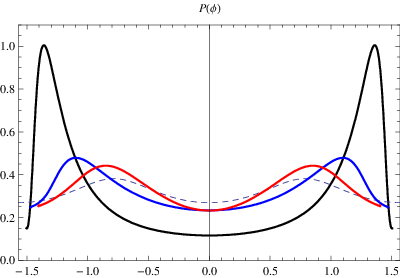
which follows immediately from Eq.(38) for the generating function at . Eq.(51) is equivalent to the recursive Eq.(22) in Ref.[14]. For weak disorder the stationary (site-independent) solution can be found analytically ( see Ref.[15] and a brief discussion in Sec.5). Examples of the distribution functions for different strength of disorder and different energies obtained by straightforward numerical solution of Eq.(51) are presented in Fig.1 (for which corresponds to the rational with the smallest denominator) and Fig.2 (for the irrational ).
The important relation Eq.(50) establishes an exact correspondence between the generating function and the probability distribution function for the phase . This identity will be used later for the proper normalization of the constructed “stationary” (site-independent) solution . It shows also that the generating function contains much more information about the system than . This is the reason why the problem of our interest – calculation of the statistical moments of normalized eigenfunctions, Eqs.(8), (37), determined by the whole – is much more difficult than calculation of the Lyapunov exponent and similar quantities determined merely by . To emphasize the difference between the two problems we note that the generalized IPR, Eq.(37), is not linear but bi-linear in . Hence the generating function itself cannot be considered as a joint probability distribution function of and . The problem of finding the joint probability distribution is not simple (see section 4.2), and involves, as the first step, the calculation of the moments for integer . This will be our main goal in this paper.
3.4 Averaged density of states
For completeness, we apply the developed formalism to derive an expression for the averaged local density of states (LDOS), determined by
| (53) |
Using the representation Eq.(16) for the retarded Green’s function, definitions Eqs.(20), (20), and relation Eq.(24), we obtain
| (54) |
Similar to the derivation of Eq.(37), we use the definition Eq.(28), relation Eq.(26): , integrate over , and take the limit , to represent Eq.(54) in the form
| (55) |
In variables, Eq.(33)-(34), the above expression reads
| (56) | |||||
4 Weak disorder. Differential equation for the generating function
An exact integral equation Eq.(38) contains all the information about local statistics of eigenfunctions at any uncorrelated on-site disorder. However, only at weak disorder the statistical anomalies we are focusing at in this paper are sharp. The point is that the region in the energy (or in the parameter ) where statistics is anomalous is proportional to [15], and for strong disorder the anomalies are rounded off. That is why in what follows we consider only the case of weak disorder .
For the case of a weak disorder, , when the “bare” (i.e.the one for the continuous model)) localization length , the “typical” squared amplitude of localized eigenfunctions and the exponential factor in front of the integral in Eq.(38) can be expanded in powers of . From now we will introduce a re-scaled variable
| (57) |
keeping the notation for the function of this variable.
4.1 Expression for moments and DOS in case of weak disorder
At weak disorder one can replace in Eqs.(37) and (56) by a -function and perform integration over . Using Eq.(5) one observes that vanishing of the argument in the -function results in
| (58) |
from where it follows that
| (59) |
As a consequence, , and we arrive at the following expression for moments
| (60) | |||||
Here we have neglected a small (at ) exponent and used the freedom of shifting the integration interval (as long as it equals to the period of the integrand). In a similar way we find from Eq.(56) the averaged DOS in the weak disorder limit:
| (61) |
Up to notations, this relation between DOS and the phase probability distribution coincides with that derived in a different way in [14]. For a long chain and far from its ends, the function becomes site-independent and the averaged local DOS coincides with Eq.(9).
4.2 Joint probability distribution function
By definition, the moments are expressed via the probability distribution function as follows:
| (62) |
where the function is yet to be found. Starting from Eq.(60), we first represent it in the form
| (63) |
which determines a “joint probability distribution function” ”. This function allows to find an average of an arbitrary function
| (64) |
thus providing a more detailed information as compared to . The connection between the two distribution functions is given by:
| (65) |
Now, we will show that the joint probability distribution function can be expressed via the basic object of our study, the generating function . Using in Eq.(60) the representation
| (66) |
integrating in by parts, and changing , we represent Eq.(60) in the form Eq.(63), where is given by
| (67) |
Eqs.(63) and (65) suggest an interpretation of the relation as a decomposition of a fast varying (from site to site) eigenfunction in terms of two auxiliary slow variables and . The joint distribution function , Eq.(67), allows one also to study separate distribution functions of these variables,
| (68) |
There is an interesting open question about a relation between the just defined distribution function of the eigenfunction phase for a finite chain with the boundary condition at its both ends, and the distribution function of the Lyapunov phase for a semi-infinite chain. These questions go beyond the scope of the current paper.
What we want to emphasize again at the end of this section is that the complete information about the system is conveniently encoded in the generating function . Our nearest task is to obtain and solve a differential equation (in the weak disorder limit) for this function.
4.3 Recursive differential operator for the generating function
For weak disorder (), the function in Eq.(38) is strongly peaked at and the integration over is effectively restricted to a narrow vicinity of . Expanding the remaining part of the integrand in powers of and keeping only the first order terms in , we represent Eq.(38) in the form:
| (69) |
where is the second order differential operator
| (70) |
The coefficients in Eqs.(69) and (70) are all combinations of and and at first glance do not show any nice structure:
| (71) |
Note that in the leading order in the disorder strength Eq.(69) depends only on the variance of the on-site disorder distribution through the bare localization length given by Eq.(57).
From Eq.(69) and the established relation Eq.(50), we can immediately write a recursive equation for the phase distribution function :
| (72) |
where
| (73) |
Equations (69) and (72) are the functional rather than the differential equations because of the different phase arguments in the left- and right-hand sides.
4.4 Differential equation at rational
In Eqs.(69) and (72) the phase argument experiences a finite jump at the transition from the site to . When with a natural and , then after transitions the shift of the phase argument becomes multiple of and the functional equations can be safely reduced (at weak disorder ) to the differential ones due to the periodicity of , Eq.(36). Thus, iterating Eq.(69) times we get a closed equation for :
| (74) | |||||
Keeping only first order terms in the disorder strength , we obtain:
| (75) |
Here the result of summation is extremely sensitive to the particular value of and this is the formal reason of an emerging anomaly. Indeed, the functions Eq.(71) contain only terms , , and , for which we have
| (76) |
Thus, for (i.e., ), only -independent parts of the coefficients Eq.(71) survive in Eq.(75). Assuming , expanding the L.H.S. of Eq.(75), and introducing the “continuous” dimensionless coordinate along the chain, we obtain:
| (77) |
The variables and are separated and one can immediately find a “stationary” (i.e. independent of ) solution
| (78) |
This zero mode solution describes the limit of a long chain with the length , it is the only one which survives at distances . This solution has been earlier obtained [10] in the continuous limit (). It also arises in the theory of a multi-channel disordered wire [19, 3]. As follows from Eq.(77), non-zero modes decay at distances providing so called “phase randomization”: the zero-mode solution corresponds to the absolutely isotropic distribution of the phase .
The corresponding moments () are found from Eq.(60) and are equal to:
| (79) |
The solution Eq.(78) corresponds to the following probability distribution of squared wave functions () in a long strictly one-dimensional system (amazingly, this result was not known before):
| (80) |
where is the chain length. Note that the distribution Eq.(80) is not normalizable, as the normalization integral is logarithmically divergent [23]. This divergency is an artefact of the zero-mode approximation and is typical to exponentially localized wavefunctions. The point is that the eigenfunction statistics changes drastically for very small values of the amplitude , where the zero-mode approximation no longer applies. This is related with the fact that the envelope (i.e. averaged over oscillations) of the typical localized wave function cannot be significantly smaller than . The smaller values of the amplitude are due to oscillations and nodes of wave functions which probability is different from that of the envelope. In the exact, -dependent distribution function the logarithmic divergency of the normalization integral is cut at .
5 Center-of-band anomaly,
As is seen from Eq.(76) for , terms survive in Eq.(75). This leads to a drastic modification of the phase-isotropic equation Eq.(77):
| (81) | |||||
where the differential operator depends explicitly on . The variables and are not separable anymore, which results in an emergent center-of-band () anomaly: the generating function and the phase distribution function become non-isotropic in . The variables and cannot be separated even for the stationary variant of Eq.(81) describing the zero mode:
| (82) |
Yet, due to a hidden symmetry of Eq.(81), a proper choice of coordinates allows to separate variables in the stationary (zero mode) equation Eq.(82). This will be done in the next subsection.
For completeness, we conclude this subsection by derivation of an exact expression for the stationary distribution function of phase (see Eq.(50)). Taking the limit in the stationary variant Eq.(82) of Eq.(81), we obtain the ordinary differential equation:
| (83) | |||||
The only periodic solution to this equation has the form [15]:
| (84) |
where the normalization constant provides the equality . Thus, the distribution of the Lyapunov phases in a long weakly disordered chain at the center of band () is not isotropic but has maxima at . According to the interpretation Eq.(39) of the amplitude-phase variables, this implies the tendency towards smaller difference between and , i.e. larger localization length. This phenomenon has been coined as “the center-of-band-anomaly”.
Now we proceed with our much more difficult task: solving not an ordinary but the partial differential equation (81) for the generating function of two variables.
5.1 Hidden symmetry and separation of variables
The integrability of the stationary equation (82) is shown in three steps. The step one is to pass from to a new set of variables with , and to introduce a new function
| (85) |
In these variables the zero-mode equation Eq.(81) takes a very symmetric form:
| (86) |
It is remarkable that the L.H.S. of this equation can be represented as where the operators and belong to the family of three operators from the representation of the algebra:
| (87) |
with the commutation relations:
| (88) |
Now it is clear that there is a hidden order in a set of coefficients in Eq.(81) resulting from the symmetry. The latter frequently manifests itself in various scattering problems. However, Eq.(81) is connected with even higher symmetry. Introducing a set of three additional (mutually commuting) operators
| (89) |
we can represent Eq.(81) in the form . The operators and constitute an algebra with the commutative subalgebra and commutation relations: (see Eq.(88)), , and ; in more detail, the latter relation looks like: and
| (90) |
It is tempting to interpret as the algebra of generators of rotations () and translations () of the 3d pseudo-euclidian space . However, the question of a constructive application of this symmetry to the considered problem remains open. Below we follow a more prosaic way.
The next step is to introduce a function
| (91) |
to transform Eq.(86) to the Schrödinger-like equation for the function :
| (92) | |||
| (93) |
Finally we introduce the variables
| (94) |
It is easy to see that in these variables the operator in Eq.(92) splits into two identical one-dimensional Hamiltonians
| (95) |
where is given by:
| (96) |
Thus, in new variables Eq.(94) the partial differential equation (82) for the generating function at is separable and can be reduced to the two ordinary differential equations of the Schrödinger type
| (97) |
defined on semi-axes and , respectively. The opposite sign of the two eigenvalues guarantees the zero-energy solution to Eq.(95).
5.1.1 Distinctions from the usual quantum mechanics.
Although Eqs.(97) look like ordinary one-dimensional Schrödinger equations on a positive semi-axis, the problem we are solving is very different from quantum mechanics. A cornerstone of the latter is the Hermiticity of a Hamiltonian which insures that corresponding eigenenergies are real and the time evolution of an initial state is unitary. For singular Hamiltonians like the one in Eq.(97), this property is not given for granted. It requires vanishing the boundary term
| (98) |
which arises at integration by parts for any two quadratically integrable functions and from the Hilbert space. We will show that this condition cannot be fulfilled for the operator Eq.(96) which eigenfunctions at are constructed as a superposition of two fundamental solutions with different behaviors at
| (99) |
Here the exponents and are the roots of the secular equation . For the both solutions oscillate at and are acceptable. For the both solutions have exponentially decreasing and increasing parts at , therefore only a properly constructed superposition of the two solutions, with cancelation of the increasing part, is acceptable. In the special case , the fundamental solution is
| (100) |
while the second solution, , is unbounded and thus should be ignored. Now, considering the equation Eq.(98) with the choice (for any ) and , we find that the boundary term vanishes at while it is not zero at :
| (101) |
This means the Hamiltonian Eq.(96) is non-Hermitian in the Hilbert space which includes all the (bounded) fundamental solutions. The remedy of the usual quantum mechanics [30] to preserve the Hermiticity of singular Hamiltonians like Eq.(96) is to reduce the Hilbert space to include only one of the two types (characterizing by the exponents ) fundamental solutions. A direct consequence of such a restriction is the absence of the bound states of negative energy [30]. Indeed, as mentioned above, for only a superposition of two fundamental solutions can provide a decrease of the wave function at .
There is no such a restriction imposed on the Hilbert space in our problem where the eigenvalue plays an auxiliary role (the zero mode of Eq.(95) arises as a result of cancelation ) and does not have meaning of an observable. That is why is allowed to be complex and there is no requirement of Hermiticity of the operator Eq.(96). We will see that in contrast to quantum mechanics, bound states (decaying at ) do exist in our problem. Moreover, their spectrum is not discrete but fills a sector on the complex plane.
5.1.2 Construction of a general solution, .
Solutions with can be expressed via the Whittaker function which obeys the Weber’s differential equation (see, e.g. Ref. [24], 9.220):
| (102) |
and decays at :
| (103) | |||
| (104) | |||
| (105) |
where is the confluent hypergeometric function, and . For , the equation (96) is mapped on Eq.(102) by the following identification:
| (106) |
Note that the solution to Eqs.(97),(102) at , which decays at , contains both a part and a part at . This clearly violates the condition of Hermiticity Eq.(98) and is the reason why the singular Hamiltonian Eq.(96) does have bound states. Moreover, the spectrum of the Hamiltonian is complex, as Eq.(106) can be easily extended to complex with the convention that at and has a cut along the semi-axis . From the asymptotic of the Whittaker function
| (107) |
we find the domain on the complex plane of , where the solution Eq.(107) is decaying: , i.e., . A general solution to Eq.(92) can be built as a superposition of ”elementary blocks”
| (108) |
with the following restrictions for and : (i) ; (ii) , . These inequalities are non-strict because in the case where one of the ’s is purely imaginary the second one is real due to the condition (i) and this provides the required vanishing of the product Eq.(108) at . The relation (i) leads to the representation , with and . Choice of the upper (lower) sign means that is restricted to the IV (I) quadrant of the complex plane with ().
As a result, the general solution to Eq.(92) can be represented as a superposition
| (109) |
where are arbitrary functions (restricted by the requirement of convergency of the corresponding integrals).
We mention for completeness, that the Whittaker functions with the second index which emerges in our problem, constitute a special class. They can be expressed in terms of the parabolic cylinder functions : , which reflects the possibility of mapping the problem Eq.(97) on the problem of two “harmonic oscillators” but with an “upside down” potential for one of them. We will not explore this correspondence in the present paper.
5.1.3 Solution in the case .
For the eigenvalue , the mapping Eq.(106) becomes singular. Two eigenfunctions of the operator Eq.(96) in this simple case are elementary functions, increasing and decreasing at , respectively. The eigenfunction decreasing at is given by Eq.(100). However, as will be shown in the next section, the corresponding solution of Eq.(97)
| (110) |
does not meet physical requirements of smoothness of as a function of and thus it must be ignored.
5.1.4 Problem of degeneracy of the general solution.
Note that Eq.(109) possesses a huge degeneracy, due to an arbitrary choice of the functions . This is in contradiction with an intuitive expectation that the statistics of wave functions in an infinite disordered chain should be unique and independent of the boundary conditions. Below we show that the natural physical requirement of smoothness of as a function of helps to determine the solution for the generating function up to a constant pre-factor which can be further fixed using the relation Eq.(50) and the normalization condition for the anomalous phase distribution function .
6 Resolving the degeneracy problem and determining the solution for the generating function
6.1 Requirements for the generating function
The stationary generating function
| (111) |
which determines the moments Eq.(60), should obey the following requirements:
1. It should vanish at .
2. It should be periodic in (with the period ). Moreover, for the considered case () the coefficients of Eq.(81) are periodic functions with the period and we impose the requirement on the stationary solution, too.
4. should be a smooth function of together with all the derivatives with respect to . It should have no jumps, cusps, etc.
The first requirement has been fulfilled due to the proper choice of the integration domains in Eq.(109) on the complex plane . The second requirement is equivalent to and can be achieved by the symmetrization of the integrand in Eq.(109) with respect to the replacement . The third requirement will be fulfilled by the properly chosen behavior of the functions at (see subsection 6.3 and Appendix A). Accounting for the fourth, extremely important requirement is not as simple. It will be postponed till subsections 6.3, 6.4.
6.2 From plane to contour integral
Similarly to the usual coherent states, the set of partial solutions Eq.(108) is overcomplete, and actually the 2d integration domains in Eq.(109) (i.e., the first and the fourth quadrants of the complex plane ) can be reduced without losses to a 1d integration contour. Consider, for instance, the first term in Eq.(109). Note that is a holomorphic function of in the first quadrant, i.e., depends only on () but not on . In polar coordinates we have:
| (112) |
where the integration contour coincides with the semi-axis , and the second equality is the realization of the possibility to rotate the contour , provided that the first argument of the function remains in the first quadrant. For instance, if we choose the contour as a ray which corresponds to the rotation of by the angle , the variable on is represented as . Changing, at a fixed , the variable in the internal integral: , where real runs from to , we arrive at:
| (113) |
where we have changed the order of integrations, introduced a new weight function
| (114) |
and changed back the notation . Thus without loss of generality we have expressed the double integral over the first quadrant in terms of a contour integral
| (115) |
Note again, that the key condition for this transformation is a holomorphic dependence of on .
Another choice of the integration contour can make the expression more symmetric. Namely, rotating the contour by the angle , so that , and introducing a new real variable by , we obtain (omitting the prime and re-defining the arbitrary function )
| (116) |
Here , .
Following the same route we obtain a contour integral representation for the second term in Eq.(109):
| (117) |
with related with .
Eqs.(116) and (117) determine the generating function Eq.(111):
| (118) |
Here we took to make the integrand symmetric with respect to the permutation in order to fulfill the formulated above requirement 2; the function is a real (without loss of generality) function yet to be determined. Up to now we have used only the following loose assumptions on its properties:
. has no singularities in the first quadrant of the complex plane;
. at , the integrand in Eq.(118) decays faster than ; this justifies rotations of the contour neglecting contributions of distant arcs.
6.3 Equation for
We begin by determining the behavior of the function at . To this end we note that according to the relations Eqs.(50) and (84), the generating function Eq.(118) must tend to a finite limit as and .
Re-scaling in Eq.(118) the integration variable , we find at
| (119) |
To provide a finite value of the expression (119) in the limit of vanishing , we should require that (see Appendix A):
| (120) |
A crucial role in further restricting the possible choice of the function is played by the requirement of smoothness of as a function of (requirement 3 of the previous subsection). The generating function Eq.(118) is periodic in with the period and it is continuous at the end points (i.e. ), and (i.e. ) of the interval of the periodicity . This is guaranteed by the c.c. term in Eq.(118), equivalent to the permutation . What is not automatically guaranteed is that is smooth as a function of at and ; the smoothness implies the continuity of all the derivatives. Amazingly, the requirement of smoothness is sufficient to determine the function up to a constant pre-factor. As we will see this happens because of the special property of the solution Eq.(118) encoded in the certain identity for the confluent hypergeometric functions in Eqs.(103)-(105).
Consider, for instance, the behavior of at , (i.e. , while ). A discontinuity of derivatives at may arise from the branching of the expression in Eq.(118) at small . Indeed, according to the representation of the Whittaker function Eq.(103) in terms of -functions Eqs.(104) and (105), we see that
| (121) |
where and are analytic functions of in the vicinity of . The common factor is canceled by the pre-factor in front of the integral in Eq.(118). The first term in the square brackets of Eq.(121) is regular in the vicinity of , while the second one , is not analytical at . As such a non-analytical behavior is in conflict with the requirement of smoothness (section 6.1), the corresponding part of the solution must identically vanish. Extracting this singular ( in the domain ) part of the general solution Eq.(118), we obtain:
| (122) | |||||
which should be fulfilled for any . Vanishing of is equivalent to the homogeneous integral equation for the real weight function with the boundary condition .
Similarly, the presence of non-analytical terms and in the special solution Eq.(110) is the reason why this solution should be ignored.
The integral equation Eq.(122) imposes severe constraints on the function , because Eq.(122) must be satisfied for arbitrary and (at ). That is why the requirement of smoothness lifts a huge degeneracy and arbitrariness in the possible choice of . The existence of even a single (non-zero) solution for is not evident. We will show below that the solution to Eq.(122) does exist and is unique up to the constant pre-factor.
6.4 Solution for
Rotating the integration contours independently for each of the two terms in the integrand of Eq.(122) and changing and , respectively, one can make the Whittaker function real and take it out of the square brackets. Thus, the integral equation Eq.(122) takes the form
| (123) | |||||
where the dependence of the integrand on and is factorized. The only possibility to satisfy this equation for arbitrary and is to require the square bracket to vanish identically.
The crucial observation for the possibility to fulfil this condition is an identity for the confluent hypergeometric functions [24]:
| (124) |
With the help of Eq.(124), we find that the square bracket in Eq.(123) vanishes identically for all if and only if the function obeys (for positive ) the condition
| (125) |
Now one can immediately guess a solution for :
| (126) |
It is easily seen that the solution Eq.(126) obeys the both conditions formulated at the end of the subsection 6.2. The function (see definition (120)) is an analytical function in the domain of our interest (). Though grows at , one can check that the integrand in Eq.(118) decays as for . This provides the convergence of the integral Eq.(118) at large and justifies rotations of integration contours neglecting contributions of infinitely remote arcs. Note also that is real at the semi-axis .
Now, looking for a general solution to Eq.(125) in the form
| (127) |
we obtain the following functional equation for at :
| (128) |
The function is also supposed to be an analytic function at . Equation (128) requires to be an analytical function of :
| (129) |
Therefore, being regular in the domain (it is even sufficient to require analyticity within a sector ), the function must be regular on all the complex plane , i.e. it should be an entire function. Now we apply the condition of convergence of the integral over in Eq.(118) at large to find the allowed asymptotic behavior of at . Substituting Eq.(127) into Eq.(118) and using the asymptotics of the Whittaker and -functions we find that the integrand behaves as at . This means that should increase not faster than . There is only one such entire function with the structure of Eq.(129): this is a constant . Thus we have proven the uniqueness of the solution Eq.(126) up to a constant factor. This factor has to be determined from the relation Eq.(50) and the normalization condition for the phase distribution function . Now we may write down the solution for the anomalous (at the center of the band) generating function in the final form :
| (130) | |||||
where , ; , . In the appendix we demonstrate explicitly that the obtained solution Eq.(130) does obey the relation , where is given by Eq.(84).

The 3D plot of the function is given in Fig.1. In the next section we apply the solution Eq.(130) for studying moments of the wave function distribution.
7 Moments of the wave function distribution
The exact expression Eq.(130) for the anomalous (at the center of the band) generating function is our main analytic result. It determines statistics of wave function distribution at the center-of-band anomaly. Although extensive physical applications go beyond the framework of the present work, here we briefly discuss the applicability of the one-parameter scaling description for the anomalous statistics.
As has been mentioned in the introduction, the Lyapunov exponent , Eq.(6), sharply decreases in a narrow vicinity of the band center [14, 15]. Being dependent only on the phase distribution function, the Lyapunov exponent can be easily calculated using Eq.(84) at the center-of-band anomaly and the trivial homogeneous phase distribution close to but outside the anomalous region. The ratio of real parts of the two corresponding Lyapunov exponents and is given by [14, 15]:
| (131) |
According to Eq.(6), this can be interpreted as an increasing localization length at the anomaly: . Note that the localization length defined via the Lyapunov exponent characterizes the exponentially decaying tails of the localized wave function and for this reason will be referred to as the ”extrinsic” localization length. In contrast to that we consider the ”intrinsic” localization length defined via the moments of the inverse participation ratio
| (132) |
whenever is independent of in a sufficiently wide interval of . This localization length characterizes the ”body” of the localized wave function.
Comparing Eqs.(79) and (132) one concludes that away from anomaly the extrinsic and intrinsic localization lengths coincide and are both equal to given by Eq.(7). To study a relationship between them at the anomaly, we analyze the behavior of moments () of the anomalous (at the center of band, , ) wave function distribution. With the definition Eq.(57), the expression Eq.(60) in the limit of a long chain takes the form:
| (133) |
where the ratio is given by Eq.(61):
| (134) |
One might expect that the behavior of anomalous moments is similar to Eq.(79) but with the localization length replaced by some other length scale . This would be the scenario of one-parameter scaling which appears to fail at the band center.
A convenient way to present the results is to plot the reduced moments (where , Eq.(60), are the moments away from the anomaly):
| (135) |
Equation Eq.(135) with taken from Eq.(134) and given by Eq.(130) is parameter-free.
First of all we check that as normalization of wave functions requires. Applying to Eq.(135) the relation (with ):
| (136) |
and using Eq.(134) one immediately obtains
.
| 1 | 2 | 3 | 4 | 5 | 6 | 7 | 8 | 9 | 10 |
|---|---|---|---|---|---|---|---|---|---|
| 1.0000 | 0.8347 | 0.6703 | 0.5321 | 0.4252 | 0.3467 | 0.2908 | 0.2519 | 0.2255 | 0.2083 |
The moments with , are essentially governed by the -dependence of the generating function . We evaluated numerically the reduced moments up to . The results are given in Fig.2 and Table 1.

One can see that the behavior of reduced moments with relatively small (), , is, indeed, compatible with Eq.(132). The best exponential fit gives the same tendency of increasing the localization length at the anomaly as in Eq.(131). However, at the anomaly the extrinsic and intrinsic localization lengths are no longer equal to each other, as it is the case at energies away from the anomaly:
| (137) |
Even more interesting phenomenon takes place for large moments. At one can see a significant enhancement of the moments compared to their value extrapolated from the exponential dependence of at small . A possible physical meaning of these new regime is discussed in a short publication [29].
8 Conclusions and open problems
Eq.(130) is the main result of the paper. It gives an exact and unique stationary (i.e. site-independent) solution (in quadratures) to the partial differential equation Eq.(81) for the generating function at the center of the energy band (, ) of a weakly disordered chain. The variables and are associated with slowly varying (squared) amplitude and phase of wave functions. The generating function we obtained can be used to compute all local statistics of normalized eigenfunctions in the one-dimensional Anderson model in the bulk of a long () chain. The solution of this problem goes beyond the known problem of the Lyapunov exponent and related quantities (e.g. density of states and conductance) [14, 15, 17, 18], which are completely determined by the distribution function of phase . As we have shown, is a descender of the generating function and is related with it in a simple way: (see Eq.(50)). Another important application of is that is the distribution function of a random phase of the coefficient of reflection from a semi-infinite disordered chain.
The integrability of the partial differential equation Eq.(82) for the generating function which we discovered, is a remarkable evidence of a hidden symmetry of the problem at . Although in the course of derivation we mentioned about the algebra of operators Eq.(87), which are the building blocks for Eq.(86), and about even more extended algebra Eq.(90), we did not exploit this algebraic content explicitly. What would be highly useful is to find the symmetry transformation which enables the discovered separation of variables. Moreover, the hidden symmetry which survives violation of the chiral (or sublattice) symmetry [28, 2] by on-site disorder, could be important for other systems (like edge states in Quantum Hall effect or in topological insulators) where the chiral symmetry is broken by disorder. Speculating on its nature we may surmise that this symmetry might be more naturally formulated in the three dimensional space rather than in the two-dimensional space and that it may have something to do with the symmetry of the 3d harmonic oscillator. This conjecture is fed by an analogy between our main result Eq.(130) and the expression for the Green’s function of the 3d harmonic oscillator problem [26]. The analogy concerns the parameter ( in our problem and in Ref.[26]) entering both the argument and the first index of the Whittaker functions in a mutually reciprocal way, as well as the second index of the Whittaker functions being in both cases (showing a connection with the parabolic cylinder function). Establishing this symmetry would also be useful for studying higher order anomalies at with (for the preliminary analysis of the “devil’s staircase” of these higher-order anomalies, see Ref.[27]).
We would like to note that the studied anomalies are inherent not only to the problem of a disordered chain but might occur in other physical situations where there is a periodic perturbation of random amplitude. We mention an analogy between the 1d localization and the classical system of kicked oscillator studied recently in Ref.[16]. According to this analogy the energy-dependent de-Broglie wavelength of a particle on a chain is encoded in the frequency of the oscillator while the lattice constant determines the period of the -function pulses of the external force (”kicks”), their amplitude being proportional to disorder. From this point of view, statistical anomalies arise due to sequences of several kicks with amplitudes correlated in time. Correlated amplitudes of kicks correspond to exclusive configurations of the local disorder, hence the anomalies are weak (for weak disorder) and exhibit themselves only in narrow windows around selected energies. Remarkably, the variables and , which allowed us to factorize the equation for the generating function of the Anderson model, play a role of the co-ordinate and the momentum of the kicked oscillator.
Finally, we applied the exact solution for the generating function to analyze the behavior of moments of the eigenfunction distribution at the center-of-band anomaly. We have found that relatively small moments behave similar to those outside the anomalous region but with a renormalized localization length , while the larger moments deviate significantly from this dependence. This fact together with the appreciable enhancement of the ”intrinsic” length with respect to the ”extrinsic” length (inverse Lyapunov exponent) , implies a significant change of the form of the ”average” eigenfunction at the center-of-band anomaly and simultaneously a failure of one-parameter description of eigenfunction statistics.
Acknowledgments
We appreciate stimulating discussions with A.Agrachev, B.L.Altshuler, Y.V.Fyodorov, A.Kamenev, A.Ossipov, O.Yevtushenko, and a support from RFBR grant 09-02-1235 (V.Y.). We are especially grateful to E.Cuevas and D.N.Aristov for a help in numerical calculations. A part of work was done during our stay at Kavli Institute for Theoretical Physics at Santa Barbara and during visits of V.Y. to the Abdus Salam International Center for Theoretical Physics. Support of these institutions is highly acknowledged.
Appendix A Normalization of : explicit check of the relation for Eqs. (130) and (84).
In order to take the limit in Eq.(130), we re-scale the integration variable and use the identity . Introducing a new integration variable , we arrive at the following expression for :
| (138) |
where (see [24])
| (139) | |||||
| (140) |
The latter expression is rather complicated. To find its real part one has to use nontrivial identities for the hypergeometric function. Obviously this brute force approach does not exploit efficiently the symmetry of the problem.
It is more advantageous and instructive to exploit the symmetry and perform the integration in Eq.(139) in several elementary steps. Using the representation ([24])
| (141) |
one can perform an elementary integration over in Eq.(139) arriving at
| (142) | |||||
Using the identity
| (143) |
(for real and ) and introducing new variables:
| (144) |
we obtain:
| (145) |
Re-scaling the variables and introducing the polar coordinates and as and , we get
| (146) |
where
| (147) | |||||
| (148) |
Collecting things together we arrive at the following final expression for , Eq.(138),:
| (149) |
This expression coincides with the anomalous probability distribution of phase Eq.(84) and thus proves the correct choice of the numerical pre-factor in Eq.(130).
References
References
- [1] P.W.Anderson, Phys.Rev. 109, 1492 (1958).
- [2] F.Evers and A.D.Mirlin, Rev.Mod.Phys 80, 1355 (2008)
- [3] A.D.Mirlin, Phys.Rep. 326, 259 (2000).
- [4] G.Modugno, Rep.Prog.Phys., 73, 102401 (2010).
- [5] R.E.Borland, Proc. R. Soc. A 274, 529 (1963)
- [6] B.I.Halperin, Phys.Rev. 139, A104 (1965); Adv.Chem.Phys. 13, 123 (1967).
- [7] V.L.Berezinskii, Zh.Exp.Teor.Fiz. 65, 1251 (1973)[Sov.Phys.JETP 38, 620 (1974)].
- [8] A.A.Abrikosov and I.A.Ryzhkin, Adv.Phys. 27, 147 (1978).
- [9] V.I.Melnikov, JETP Lett. 32, 225 (1980).
- [10] I.V.Kolokolov, Zh.Exp.Teor.Fiz. 103, 2196 (1993)[JETP 76, 1099 (1993)].
- [11] J.B.Pendry, Adv.Phys. 43, 461 (1994).
- [12] J.Frohlich, F.Martinelli, E.Scoppola and T.Spencer, Comm.Math.Phys. 101, 21 (1985).
- [13] I.M.Lifshitz, S.A.Gredeskul and L.A.Pastur, Introduction to the theory of disordered systems (Wiley, New York, 1988).
- [14] M.Kappus and F.Wegner, Z.Phys. B 45, 15 (1981).
- [15] B.Derrida and E.Gardner, J.Phys. (Paris) 45, 1283 (1984).
- [16] L.Tessieri and F.M.Izrailev, Phys.Rev.E 62, 3090 (2000).
- [17] H.Schomerus and M.Titov, Phys.Rev.B 67, 100201(R) (2003).
- [18] L.I.Deych, M.V.Erementchouk, A.A.Lisyansky, and B.L.Altshuller, Phys.Rev.Lett. 91, 096601 (2003).
- [19] K.B.Efetov, Supersymmetry in chaos and disorder (Cambridge University Press, Cambridge, England, 1977).
- [20] A.D.Mirlin and Y.V.Fyodorov, Nucl. Phys. B 366, 507 (1991).
- [21] R.Abou-Chacra, P.W. Anderson, and D.J. Thouless, J. Phys. C 6, 1734 (1973).
- [22] A.Ossipov and V.E.Kravtsov, Phys.Rev.B 73, 033105 (2006).
- [23] All the positive moments of this distribution are finite, in particular .
- [24] I.S.Gradshtein and I.M.Ryzhik Table of integrals series and products (Academic Press, New York, 1996).
- [25] C.Barnes and J.M.Luck, J.Phys. A 23, 1717 (1990).
- [26] V.L.Bakhrakh and S.I.Vetchinkin, Theor.Math.Phys. 6, 283 (1971) [Sov. Phys: Teor. Mat. Fiz.6, 392 (1971)].
- [27] V.E.Kravtsov and V.I.Yudson, AIP Conference Proceedings, 1134, 31 (2009). ArXiv:0806.2118;
- [28] F.J.Dyson, Phys.Rev. 92, 1331 (1958).
- [29] V.E.Kravtsov and V.I.Yudson, Phys.Rev. B 82, 195120 (2010).
- [30] L.D.Landau and E.M.Lifshitz, Quantum Mechanics, Elsevier Science Ltd. 1977.