Holographic description of large gauge theory
Abstract
Based on the earlier work [S.-S. Lee, Nucl. Phys. B 832, 567 (2010)], we derive a holographic dual for the -dimensional lattice gauge theory from a first principle construction. The resulting theory is a lattice field theory of closed loops, dubbed as lattice loop field theory which is defined on a -dimensional space. The lattice loop field theory is well defined non-perturbatively, and it becomes weakly coupled and local in the large limit with a large ’t Hooft coupling.
I Introduction
Although there are many non-trivial evidences for the anti-de Sitter space/conformal field theory (AdS/CFT) correspondence[1, 2, 3], a first principle derivation of the conjecture is not available yet. Nonetheless the correspondence has been employed to a wide range of physical systems including condensed matter systems[4, 5, 6, 7], in a hope that certain features of strongly coupled quantum field theory can be captured by holographic theories constructed based on phenomenological reasoning. On the one hand, such approaches have produced interesting insights into strongly coupled quantum many-body systems. On the other hand, there exists a clear limitation because it has not been possible to identify the precise holographic dual for a general quantum field theory that one may want to understand.
Since the ’t Hooft’s observation that large gauge theory is related to a weakly interacting string theory[8], it has been suggested that there exist intrinsic connections between the two theories[9]. The fundamental object that bridges between these two theories is Wilson loop which becomes classical in the large N limit. The dual string theory that governs the classical equation of motion of Wilson loop[10, 11] in the loop space is expected to be defined on one higher dimensional space than the space on which the field theory is defined, and the additional dimension corresponds to the energy scale in the renormalization group (RG) sense[9]. There have been many works which made the connection between RG flow of general quantum field theory and holographic theory more precise[12, 13, 14, 15, 16, 17, 18, 19, 20].
In this paper, we present a first principle construction of a holographic theory dual to the gauge theory based on the prescription[18] which has been applied to the vector model[21, 22, 23, 24, 25]. We use the lattice regularization for the gauge theory. The derived holographic theory is a lattice field theory of closed loop defined on a -dimensional lattice which can be viewed as a discrete AdS space. The holographic theory becomes classical in the large limit and locality emerges when the ’t Hooft coupling is large. This construction provides a realization of an earlier idea of reformulating large N gauge theory as a classical theory of gauge neutral fields[26, 27].
II From U(N) gauge theory to loop field theory
We start with the gauge theory defined on the D-dimensional Euclidean hypercubic lattice,
| (1) |
with the action,
| (2) |
Here is Wilson line defined on closed oriented loop ,
| (3) |
where is matrix (holonomy) defined on nearest neighbor bond , and . In Eq. (3) and all products of holonomies hereafter, we assume that the product is path-ordered along the orientation of the curve. is the sum over unordered sets of closed loops. , , … are coupling constants associated with single-trace, double-trace operators, and so on. For single trace coupling, we will also use the notation interchangeably. The factor of has been singled out from each coupling. Roughly, the inverse of corresponds to the ’t Hooft coupling. Throughout the paper, we will focus on the large limit with fixed . In this limit, the action is manifestly proportional to . To guarantee the reality of the action, we impose where is the inverse loop of , namely the loop with the same trajectory but with the inverse orientation. If one ignores all multi-trace deformations and loops larger than the unit plaquette, one restores the standard lattice gauge theory[28]. Here we consider the most general gauge invariant action. We assume that couplings associated with large loops or multi-trace couplings with loops which are far from each other are exponentially small in the size of large loops or in the separation between loops. If couplings satisfy this condition, we say the theory is local. We note that effective theories obtained by integrating out short distance fluctuations generically contain non-local terms which are exponentially small.


To set the stage for a real-space renormalization, we divide links in the lattice into two sets[29]. The first set contains links that form a coarse grained lattice, that is, the hypercubic lattice with the lattice spacing twice larger than the original one. The second set contains all other links. This is illustrated in Fig. 1. The action can be divided as
| (4) |
where holonomy on links in are denoted with tilde : if . Here and are the actions which contain Wilson loops only in and , respectively, and includes loops that span across and , as is shown in Fig. 2. Now the partition function is written as
| (5) |
where .


We note that consists of Wilson loops where parts of the loops are made of holonomy in and the remaining parts in . For example, the loop in Fig. 3 (a) represents a term
| (6) |
in , where and are two segments of the closed loop which belong to the sub-lattices and respectively. Hereafter, we will use the notation to represent that is the -th segment of a closed loop , where increases along the orientation. Accordingly, represents the holonomy along the curves . We add tilde as to represent holonomies along curves which are in . For all diagrams in Fig. 3, we have
| (7) |
These holonomies on open segments are the basic building blocks for the coupling between the two sub-lattices in . However, the present form of the coupling is not very convenient for real space RG because holonomies on open segments in each sub-lattice are not gauge invariant. Therefore it is desirable to reorganize terms in such that the gauge symmetry is more manifest in each sub-lattice, that is, is written as products of gauge invariant Wilson loops in each sub-lattice. To achieve this, we first note that the action is invariant under a ‘sub-lattice gauge transformation’ defined by
| (8) |
where is matrix. Note that this is not a part of the original gauge transformation11 1 Even though with and with share the same site only gets transformed under the sub-lattice gauge transformation. . The full action is not invariant under this transformation because includes holonomies on open segments in sub-lattice . Since the action respects the sub-lattice gauge symmetry in , only those configurations where there is no open end in survive inside . Therefore, for Fig. 3 (a) vanishes. Segments in may form closed loops by themselves as in Fig. 3 (b), in which case the average does not vanish. Non-vanishing contributions can be written as a product of Wilson loops using the formula 22 2 To prove this, consider , where , , , are color indices, while are site indices, and represents insertions of link fields which do not include the site . The color index () carry fundamental (anti-fundamental) charge of U(N) at site . Because is gauge invariant, we have for any matrix . The only singlet tensor that can be constructed from one fundamental and one anti-fundamental indices is the identity. Therefore with . From this, one obtains Eq. (9).,
| (9) |
This is illustrated in Fig. 4. We emphasize that this identity is valid only inside the average, but not as an operator identity. Using this formula, we obtain
| (10) | |||||
for Fig. 3 (b). Generally, only those diagrams where all open segments in sub-lattice form closed loops do not vanish. For Fig. 3 (c) and (d), one obtains
| (11) |
Note that if segments in sub-lattice form loops, segments in sub-lattice automatically form loops. Therefore all non-vanishing terms in can be expressed as a polynomial of Wilson loops in and ,
where depends only on , and , but not on , 33 3 When more than two Wilson loops cross at a point, one needs more general formula than Eq. (9). However, all non-vanishing contributions can be always written as products of Wilson loops.. This polynomial for and can be exponentiated as
| (13) |
where
Here is the cumulant of . Since , is in the large N limit 44 4 This is why we deliberately singled out the factor of out of .. can be computed perturbatively in and 55 5 This corresponds to a strong ’t Hooft coupling expansion in the large limit.,
| (15) | |||||
| (16) | |||||
| (17) | |||||
and so on. Here is a Kronecker delta function in the space of loops. It is easy to understand physical meaning of each term. The first term in Eq. (15) describes a loop which has a self-intersecting point as in Fig. 3 (b) decomposes into two loops and which are in and , respectively. The second term describes a two-loop state where one is included in and the other in . The third and fourth terms describe the process where two and three loops join to form a loop in and a loop in as in Fig. 3 (c) and (d), respectively. The first term in Eq. (16) describes a loop decomposing into three loops, two of which (, ) are in and one (), in through two self intersecting points. The remaining terms can be understood similarly.
We call those Wilson loops that contribute to ‘connected Wilson loops’. There are two kinds of them. Connected Wilson loops of the first kind are those that touch each other in space at crossing points where links in and meet. For example, the Wilson loops and in the first term of Eq. (15) are connected at a crossing point as in Fig. 3 (b). The second kind includes those Wilson loops that are physically separated but the separated loops originate from multi-trace couplings, such as the second term in Eq. (15), where and are in general separated in space but they are ‘connected’ through .
Now the partition function can be written as
| (18) |
where
| (19) |
This theory can be viewed as a theory defined on the lattice whose sources are dynamical, where fluctuations of the sources are provided by the dynamical degrees of freedom defined on . Since , the dynamical sources become classical in the large limit. Therefore it is useful to introduce collective fields for the source fields. We decompose and by introducing the Hubbard Stratonovich fields[18],
| (20) |
where and
| (21) | |||||
’s are fluctuating sources for Wilson loops on , and is a complex Lagrangian multiplier which imposes the constraint and its complex conjugate. With this normalization of , the equation of motion for implies . Physically, describes fluctuations of the Wilson loop operators. The dynamical action for is generated once is integrated over,
| (22) |
where
| (23) |

In order to repeat the coarse graining procedure, it is convenient to map into the same form as the original lattice. For this, we merge every two links in into one link in a new lattice as is shown in Fig. 5. Accordingly, two holonomies on merged links are combined to produce one holonomy as which is defined on the coarse grained lattice labeled by . Since the Wilson loops on depend only on , the partition function becomes
| (24) |
upto an unimportant multiplicative constant, where and
| (25) | |||||
| (26) | |||||
| (27) |
Here ’s are loops on . represents a dilatation map which takes a loop in to the original one before rescaling in as is illustrated in Fig. 5. This is necessary because and are defined on while and are defined on .

This is a theory defined on the coarse grained lattice with dynamical coupling fields , with the action . The second term in Eq. (25) is given by
| (28) |
where
| (29) |
with
| (30) |
Therefore is given by the effective potential for the gauge theory defined on the sub-lattice with the set of couplings, . In the large limit, planar diagrams give the leading contribution and is . For large ’t Hooft couplings (), it is natural to compute as a power series of in the real space[30],
| (31) |
This can be easily checked by using . Due to the Kronecker delta function, the first term survives only when . Similarly, the second term is nonzero only when the three oriented loops form a connected double-line graph with no unpaired single line. These are illustrated in Fig. 6. General contributions to are given by multiple oriented surfaces made of double lines, where each face in double line graphs is associated with . For example, and are contributions from one surface and two surfaces, respectively. Note that is non-linear in , and fluctuations of no longer impose a strict delta function for : they become dynamical fields.

This completes one step of our RG procedure. If we repeatedly apply this cycle to the theory on , and then to the coarse grained lattice of and so on, we can write the partition function as a integration over ’s and ’s[18],
| (32) |
where and are Hubbard-Stratonovich fields introduced at the -th step of coarse graining, and is fixed by the microscopic couplings,
| (33) |
Here plays the role of a discrete coordinate for the new -th dimension that corresponds to the length scale in RG; fields at small (large) describe UV (IR) physics. This -dimensional theory is a holographic theory for the -dimensional lattice gauge theory. We will call it lattice loop field theory (LLFT).
Since it is difficult to write down the full theory in a compact form, let us try to understand some general features of the theory from the first few leading terms of the action in the strong coupling expansion (). By plugging Eqs. (15)-(17) into Eqs. (30) and (31), one obtains,
where the ‘Hamiltonian’ (the reason for this naming will become clear shortly) is given by
| (35) |
where include terms that involve fields associated with multi-loop states and higher order terms in . Here indices , and are understood to be summed over loops in , and , respectively. If is a self-retracting loop, we set . LLFT is defined on the -dimensional lattice shown in Fig. 7. This lattice may be viewed as a discrete version of the anti-de Sitter (AdS) space where the continuous isometry , of the metric is replaced by a discrete scale invariance, , , if one assumes that all nearest neighbor bonds along the D-dimensional directions have the same physical length. However, we emphasize that this assumption is not generally true, and the metric is determined dynamically from the equation of motion for the loop fields. The true AdS space will emerge only if the solution respects the scale invariance. In theories which are not conformal, such as the present pure Yang-Mills theory, we expect that the infrared geometry will be effectively cut-off by the mass gap. We will defer this dynamical issue to a future study, and focus on the general structure of the theory in the following. We note that this kind of ‘discrete AdS’ space has been the natural setting for the real space renormalization group approach and the multi-scale entanglement renormalization Ansatz (MERA)[31, 32, 33]. The degrees of freedom of LLFT are fields of loops and .
It is convenient to interpret as a discrete (imaginary) ‘time’. Then we can identify the first term in Eq. () as the Berry phase term which dictates that and are conjugate to each other : loop fields as operators would satisfy the commutation relation if time was continuous. The remaining term in Eq. () is the ‘Hamiltonian’ that governs the evolution of the loop fields along the discrete time66 6 However, the analogy with Hamiltonian is not perfect because is not Hermitian.. Formally, () can be viewed as the path integration representation of an operator that annihilates (creates) a set of loops at time , and () is associated with an annihilation (creation) operator of ‘anti-loops’. It is noted that and are not the usual annihilation and creation operators because they are not Hermitian conjugate to each other. In the basis given by
| (36) |
and ( and ) become the standard annihilation and creation operators of loops (anti-loops ) respectively. However, we will use the basis of and in the following because it has two merits. First, the Hamiltonian becomes particularly simple in this basis because contains only those with : loops can be created only on those links that survive coarse graining at each step of RG. Second, the equations of motion for and implies . Therefore it is convenient to absorb into to define . At the saddle point, the Hamiltonian becomes Hermitian and the Berry phase term for and becomes that of the standard creation and annihilation operators upto the factor of . Note that the expectation value of creation operator is not in general complex conjugate of that of annihilation operator, i.e. , when the saddle point is ‘time’-dependent.
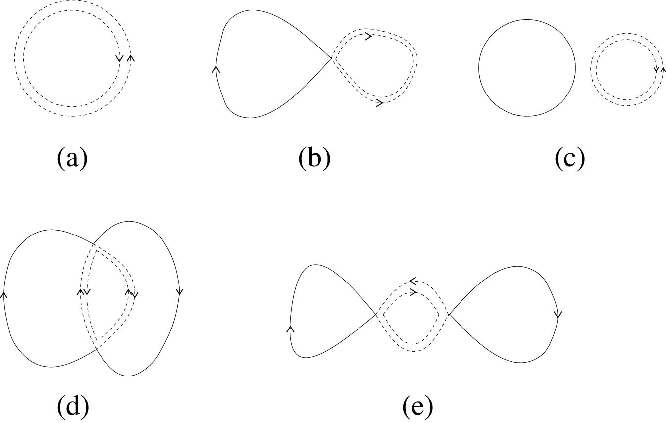
Now let us take a closer look at the Hamiltonian to understand the physical meaning of each term. The quadratic term describes a process where a loop and its anti-loop are pair-annihilated (Fig. 8 (a)). Higher order terms describe fluctuations and joining/splitting processes of loops : describes a process where a loop with a self intersection becomes a smaller loop by combining with a loop (Fig. 8 (b)); describes one of the loops in a two-loop state disappearing into vacuum with its anti-loop (Fig. 8 (c)); describes two loops merging into one loop with a help of an anti-loop which eliminates parts of the two loops(Fig. 8 (d)); describes a process where one loop gets split into two(Fig. 8 (e)).

Usually, it is expected that a quadratic kinetic energy term describes propagation of loops in space and time. Actually there is no such term in the Hamiltonian. Instead, fluctuations of loop arise only through cubic and higher order terms in and . Here we have to remember that and have nonzero expectation value in the vacuum because of the boundary condition . Therefore one has to identify and as the propagating loop fields. For these fields that describe small fluctuations of loop fields, the Hamiltonian includes the quadratic kinetic energy which describes fluctuations and propagation of loops in spacetime,
| (37) |
where is ‘hopping’ probability amplitude for a loop at time to change into a loop at time . The Hamiltonian also contains interactions between propagating loop fields. For example, the cubic interaction terms,
| (38) |
describe the processes where two loops join into one loop and one loop splits into two loops, respectively. These are illustrated in Fig. 9. In general, loops involved in hopping and interaction can be far from each other in space. However, such non-local terms will be exponentially suppressed if is small, and decreases exponentially as the size of loops increases or as the separation between the loops in multi-trace couplings increases. This is because only connected diagrams contribute to the Hamiltonian. For example, in order for a loop to hop by a large distance, there must be a large number of loops that connect the initial and final states, or there must be a multi-trace coupling that connect them. This suggests that LLFT intrinsically has non-local elements, but a sense of locality emerges if vacuum satisfies certain conditions. In a sense, locality is a property of the vacuum rather than the theory itself. We will discuss more about the condition for locality in the next section.

Is there a symmetry underlying this action ? The action in Eq. () has infinitely many conserved charges. Namely, one can define one U(1) charge for every directed link so that
| (39) |
where is a link on the original lattice (the boundary of the discrete AdS space), maps a loop on the -th coarse grained lattice to a loop on the original lattice by magnifying the loop by times ( , , …), and is the total number of times that loops pass through the link . If a loop pass the link from to (from to ), it contribute () to as is illustrated in Fig. 10. In general, any term that respects these symmetries arises in . For example, there is a term that describes a multi-loop scattering process,
| (40) |
where incoming loops become outgoing loops. Here the delta function imposes the charge conservation.
Although the action is invariant under the local symmetries, the infinite set of symmetries is broken by the boundary condition . In general, there remain only unbroken global symmetries generated by,
| (41) |
where . Conservation of implies that if a loop has a certain number of links along direction, it should have the same number of links along to form a closed loop. The conservation of means that there are only closed loops. This conserved charge is a lattice version of the charge carried by world sheet of fundamental string which is coupled to the NS-NS two form gauge field in the critical string theory.
III Classicality and Locality
The prefactor in can be identified as the inverse of ‘Planck constant’ that controls quantum fluctuations of and . Therefore the theory becomes classical in the large limit. The saddle point occurs along the imaginary axis for . The equation of motion takes the form of the Hamilton equation[13] in discrete time,
| (42) | |||||
| (43) |
The second equation needs a further explanation. In general, there is no inverse for the map because not all loops in step survives in step . If there is no inverse for , we simply define .
To solve the equations of motion, one needs two boundary conditions for each . One condition is given by Eq. (33). The other condition should be implemented dynamically, namely by minimizing the whole action over all possible paths of and subject to Eq. (33). This is analogous to the problem of finding the classical trajectory of a particle where the initial position is fixed, but the initial velocity is a variational parameter one uses to minimize the action.

Is the theory local in dimensions ? The theory is evidently local along the new dimension . The locality along the original dimensions is more tricky. This is because size of loops can be arbitrarily large. Even though one starts with small loops, multi-loop interactions generate large loops. Large loops can, in turn, mediate interactions between loops which are far from each other. Fig. 11 shows an example where two large loops and mediate interaction between two small loops and which are far from each other,
| (44) |
The non-local coupling between and is proportional to the amplitude of the large loops, . This looks bad for locality. However, if the saddle point value of decreases exponentially as the size of the loop increases, the non-local coupling is exponentially small. In this case, locality is still maintained. Therefore, we can choose the initial couplings as
| (45) |
where is the ’t Hooft coupling much larger than , is the minimum area enclosed by the loop , and is the minimum distance between the two loops. Now we prove that if the saddle point values of are exponentially small for large loops, those of are also exponentially small for large loops. Because the Hamiltonian depends on only through in Eq. (30), Eq. (42) can be written as
| (46) | |||||
where we used
| (47) |
Note that carries charges for loops, and . Therefore, if any loop in is large there must be a large number of ’s or at least one with a large loop in in order to match the charge. Similarly, if there are two loops in which are far from each other, must include either a large number of loop fields or at least one multi-loop fields such as where the separation between and is large which connect the separated two loops. This is because disconnected diagrams do not contribute to . This guarantees that if the condition in Eq. (45) is satisfied for a large at time , a similar set of condition will be satisfied with a large at time . Therefore the theory will remain local as far as the theory stays strongly coupled with large ’t Hooft couplings along the renormalization group flow. This is certainly true for small (UV region) if one starts with large ’t Hooft couplings.
Whether the amplitudes for large loops remain exponentially small for large (IR region) will be determined dynamically through the equation of motion. Here we can think of three possibilities. The first possibility is that the energy dependent ’t Hooft coupling increases without a bound as increases. In this case, the locality becomes better at IR. On the other hand, fluctuations of loop fields become suppressed and loops become very heavy in the IR limit. This is the case for the pure gauge theory in the strong coupling limit . In the low energy limit, there is no light degrees of freedom, which describes the confinement phase. The second possibility is the case where decreases to a small value in the IR limit. If this happens, non-local couplings between loops become significant below a certain energy scale (). In this case, the theory becomes non-local in the IR limit. This occurs if the theory flows to a IR fixed point which is not strongly coupled, that is, . The last possibility, for which the holographic description is most useful, is that the ’t Hooft coupling stays at a large but finite value in the large limit. This can be realized in a theory which flows to a strongly interacting conformal field theory, such as the super Yang-Mills theory at a large ’t Hooft coupling. Then the IR dynamics is described by a weakly interacting local theory of closed loops. At the saddle point, loop fields generically have nonzero expectation values. Small fluctuations of loop fields around the classical configuration will be described by a perturbative string theory. However, LLFT is well defined even non-perturbatively, and one can consider non-perturbative objects such as solitons.
IV Discussions
IV.1 Relation between LLFT and string field theory
One may view LLFT as a string field theory put in lattice. In order to obtain a string field theory in the smooth AdS space, it would be better to use a different regularization for the gauge theory. This is because RG steps can not be continuous in the lattice regularized theory. It would be of interest to devise a better regularization scheme for strongly coupled gauge theory which allows one to construct a more cut-off independent holographic theory. However, the lattice construction will be more useful to describe non-critical phases in real lattice models.
IV.2 Comparison with the vector model
The equation of motion in Eqs. (42) and (43) can be solved only if another boundary condition is provided besides the UV boundary condition in Eq. (33). The extra boundary condition should be imposed dynamically in the IR limit. In the case of the holographic vector model[18], imposing the IR boundary condition amounts to solving the original field theory. Because the holographic theory for the model has non-singlet bulk fields which are not classical even in the large limit, one has to integrate over the non-singlet bulk fields in the IR limit to dynamically impose the second boundary condition. On the other hand, in the gauge theory only singlet fields are physical and all bulk degrees of freedom are classical in the large limit. For this reason, the IR boundary condition can be imposed by minimizing the whole action with respect to the loop fields in the IR limit. Whether this leads to a simple regularity condition as in the standard AdS/CFT correspondence is yet to be understood. Nonetheless, in large gauge theory, everything boils down to solving classical problem, which is the major difference from the model. Therefore, the duality between LLFT and the large gauge theory is a strong-weak coupling duality, contrary to the case for the vector model.
IV.3 Outlook
Here, we comment on some advantages and disadvantages of the present approach which is rather orthogonal to earlier ones. First, the present prescription is general, and it can be applied to general quantum field theories. Holographic duals constructed in this way are not expected to be very useful for quantum field theories for which the dual descriptions involve strong coupling or non-locality. However, the strategy would be to establish a prescription applicable to general field theories, and then investigate how classical limit and locality emerge as dynamical features of certain theories. Second, dual theories constructed in this prescription has full quantum actions in the bulk. The correspondence is beyond the level of matching equations of motion in the bulk with beta functions of field theories. Only in the large N limit, the classical equation of motion in the bulk can be directly compared to the beta function of the boundary theories. This is an aspect in which the present approach clearly differs from the standard Wilsonian RG. Third, the basic bulk degrees of freedom in this approach are fluctuating sources and vacuum expectation values of operators in terms of which the standard AdS/CFT conjecture has been formulated.
The present approach also has some disadvantages. First, the diffeomorphism invariance is not manifest. Since the bulk space is emergent, it is expected that there should be a redundancy in parameterizing the space. Choosing a different gauge would amount to choosing a different prescription of real space RG, such as coarse graining degrees of freedom at different rates at different points in space. In the present formalism, the gauge redundancy is not manifest because specific ‘time’ slices are chosen. To make the diffeomorphism invariance more explicit, it may be useful to integrate in pure gauge degrees of freedom in the formalism based on continuous RG step. Second, there is a large number of non-dynamical fields in the bulk. In gauge theory, one has to keep infinitely many loop fields associated with multi-trace operators even for a finite . Although this issue is less acute in the large limit, it would be interesting to explicitly remove non-dynamical fields from the beginning. This is in contrast to the O(N) vector model where one needs to introduce only a finite number of fields in the bulk[18].
V Acknowledgment
I would like to thank Alex Buchel, Hong Liu, Keith Ng, Joao Penedones, Eva Silverstein, Brian Swingle and Mithat Unsal for helpful comments and discussions. This research was supported in part by the Natural Sciences and Engineering Research Council of Canada and the Early Research Award from the Ontario Ministry of Research and Innovation. Research at the Perimeter Institute is supported in part by the Government of Canada through Industry Canada, and by the Province of Ontario through the Ministry of Research and Information.
References
- [1] J. M. Maldacena, Adv. Theor. Math. Phys. 2, 231 (1998).
- [2] S. S. Gubser, I. R. Klebanov and A. M. Polyakov, Phys. Lett. B 428, 105 (1998).
- [3] E. Witten, Adv. Theor. Math. Phys. 2, 253 (1998).
- [4] S. A. Hartnoll, Class. Quant. Grav. 26 224002 (2009) [arXiv:0903.3246 [hep-th]].
- [5] C. P. Herzog, Phys. A 42 343001 (2009) [arXiv:0904.1975 [hep-th]].
- [6] J. McGreevy, arXiv:0909.0518.
- [7] S. Sachdev, arXiv:1002.2947.
- [8] G. ’t Hooft, Nucl. Phys. B 72, 461 (1974).
- [9] A. M. Polyakov, Nucl. Phys. Proc. Suppl. 68, 1 (1998); A. M. Polyakov, Int. J. Mod. Phys. A 14 645 (1999).
- [10] A. Polyakov Nucl. Phys. B 164, 171 (1980).
- [11] Y. Makeenko and A. Migdal, Nucl. Phys. B 188, 269 (1981).
- [12] E. T. Akhmedov, Phys. Lett. B 442, 152 (1998); E. T. Akhmedov, hep-th/0202055.
- [13] J. de Boer, E. Verlinde and H. Verlinde, J. High Energy Phys. 08, 003 (2000).
- [14] M. Li, Nucl. Phys. B 579, 525 (2000).
- [15] S. R. Das and A. Jevicki, Phys. Rev. D 68, 044011 (2003).
- [16] R. Gopakumar, Phys. Rev. D 70, 025009 (2004); ibid. 70, 025010 (2004).
- [17] I. Heemskerk, J. Penedones, J. Polchinski and J. Sully, J. High Energy Phys. 10, 079 (2009).
- [18] S.-S. Lee, Nucl. Phys. B 832, 567 (2010).
- [19] I. Heemskerk and J. Polchinski, arXiv:1010.1264.
- [20] T. Faulkner, H. Liu and M. Rangamani, arXiv:1010.4036.
- [21] I.R. Klebanov and A.M. Polyakov, Phys. Lett. B 550, 213 (2002).
- [22] M. A. Vasiliev, arXiv:hep-th/9910096.
- [23] A. C. Petkou, J. High Energy Phys. 03, 049 (2003).
- [24] S. Giombi and X. Yin, arXiv:0912.3462.
- [25] R. Koch, A. Jevicki, K. Jin and J. P. Rodrigues, arXiv:1008.0633.
- [26] E. Witten, “The 1/N expansion in atomic and particle physics, in Recent developments in gauge theories,” eds. G. ’t Hooft et al., Plenum, 1980, p.403.
- [27] S. Coleman, “1/N,” in Proc. of Erice Int. School of Subnuclear Physics 1979, Plenum, N.Y., 1982, p. 805.
- [28] K. G. Wilson, Phys. Rev. D 10, 2445 (1974).
- [29] E. Fradkin and S. Raby, Phys. Rev. D 20, 2566 (1979).
- [30] I. Bars and F. Green, Phys. Rev. D 20, 3311 (1979).
- [31] G. Vidal, Phys. Rev. Lett. 101, 110501 (2008).
- [32] Z.-C. Gu, M. Levin and X.-G. Wen, Phys. Rev. B 78, 205116 (2008).
- [33] B. Swingle, arXiv:0905.1317.