A new viable region of the inert doublet model

Above the $W$ threshold, $M_{H^{0}}>M_{W}$, dark matter annihilation into $W^{+}W^{-}$ becomes kinetimatically allowed, with the result that the total annihilation cross section tends to be rather large. If we estimate it from the pure gauge diagram –figure 1, (a)–, we get that

which, for $M_{H^{0}}\sim 100~\mathrm{GeV}$, gives about $2\times 10^{-24}\mathrm{cm^{3}/s}$. And a similar number is found for the annihilation into $Z^{0}Z^{0}$. These annihilation cross sections are both much larger than those required to obtain the correct relic density ($\sigma\mathrm{v}\sim 3\times 10^{-26}\mathrm{cm^{3}/s}$), so it seems difficult to satisfy the dark matter constraint in this mass range. In fact, previous analysis have claimed that it is not possible to do so. In [13], they stated that the inert Higgs could only provide a subdominant component of the dark matter, while in [14] they found the relic density to be too suppressed to be consistent with WMAP unless $M_{H^{0}}>600~\mathrm{GeV}$.

Here, we show that those conclusions are incorrect. Taking advantage of the interference among the different diagrams that contribute to dark matter annihilation into gauge bosons, it is possible to satisfy the relic density constraint for $M_{H^{0}}\gtrsim M_{W}$. Thus, opening up a new viable region of the inert doublet model.

Let us now explain how these interference effects come about. The diagrams that contribute to dark matter annihilation into $W^{+}W^{-}$ (or $Z^{0}Z^{0}$) are shown in figure 1. Their amplitudes are given by

where $\epsilon_{\mu}^{*}(p)$ is the polarization vector of the gauge boson with momentum $p$, $p_{1}$ and $p_{2}$ are the momenta of the $H^{0}$’s, and $s$, $t$ and $u$ are the Mandelstam variables. In these equations, $g_{V}=g,g/\cos\theta_{W}$ and $\chi=H^{\pm},A^{0}$ respectively for the annihilations into $V=W^{\pm},Z^{0}$. Typically, the first two contributions (the point-like interaction and the Higgs-mediated diagram) dominate the total annihilation cross section, so we will focus on those in our analytical discussion. Far from the Higgs resonance, their squared amplitude can be written as

Since $s\simeq 4M_{H^{0}}^{2}$ at low velocities, a cancellation between the two contributions occurs for

to which we refer as the cancellation condition. Hence, cancellations take place for $\lambda_{L}>0$ if $M_{H^{0}}<M_{h}/2$ and for $\lambda_{L}<0$ if $M_{H^{0}}>M_{h}/2$. For example, in the case of $M_{H^{0}}=120$ GeV and $M_{H^{0}}<M_{h}/2$, cancellations occur for $\lambda_{L}\simeq(0.04,0.5,1.2,2.0)$ when $M_{h}\,=(250,350,450,550)$ respectively, while for $M_{H^{0}}>M_{h}/2$, cancellations should occur for $\lambda_{L}\sim[-0.35,-0.1]$ when $M_{h}\,\in\,[121,200]$. Notice also, that the cancellation condition is the same for both final states, $W^{+}W^{-}$ and $Z^{0}Z^{0}$, indicating that both processes will be simultaneously suppressed. The idea, then, is that in regions of the parameter space where the cancellation condition is satisfied, the annihilation rate could be much smaller and, accordingly, a larger relic density will be found. Perhaps, large enough to be compatible with WMAP.

The existence of cancellations in the annihilation cross section into gauge bosons had already been noticed in [17] and in [20]. But the possibility of using them to obtain viable models above $M_{W}$ had not been considered before.

Let us also emphasize that the $t$- and $u$-channels that we have neglected in the above analysis will certainly affect the annihilation cross section into $W^{+}W^{-}$ and $Z^{0}Z^{0}$. We will see that in order to comply with the relic density constraint it is necessary to suppress their contributions by considering large values of $M_{A_{0}}$ and $M_{H^{\pm}}$.

Suppressing the annihilations into $W^{+}W^{-}$ and $Z^{0}Z^{0}$ is not enough to ensure a small dark matter annihilation cross section. In addition, we must make sure that the other relevant annihilation final states, that is $hh$ and $t\bar{t}$, do not give a large contribution to it. If $M_{H^{0}}>M_{h}$, the total s-wave contribution to the $H_{0}H_{0}\rightarrow hh$ annihilation process is given by

Using $M_{H^{0}}\gtrsim M_{h}$ and the $\lambda_{L}$ of equation (20), we obtain that $\sigma v_{hh}^{\rm(s-wave)}$ is typically of ${\cal O}(10^{-23})\mathrm{cm^{3}/s}$, giving rise to a very suppressed relic abundance. To be compatible with the observed dark matter density, then, the mass of the dark matter particle must be smaller than the Higgs mass ($M_{H^{0}}<M_{h}$), so that the annihilation channel into $hh$ is not kinematically allowed. This limitation of the parameter space is not that strong in the inert doublet model, for the Higgs mass can be quite large. A very stringent constraint comes instead from the annihilation into $t\bar{t}$. The total s-wave contribution to the $H_{0}H_{0}\rightarrow t\bar{t}$ process is given by

where $m_{t}$ is the top mass and $N_{c}=3$ is the color factor. Again we find that the $\lambda_{L}$ satisfying the cancellation condition yields a very small relic abundance for $M_{H^{0}}\gtrsim m_{t}$. Therefore, viable models must feature $M_{H^{0}}<m_{t}$. In [33], for instance, it was assumed that $M_{H^{0}}\gg m_{t},M_{h}$, so the effect of cancellations was overlooked in their study. As a result, the minimal value of $M_{H^{0}}$ consistent with WMAP was found to be $535~\mathrm{GeV}$. From our analysis of the mass range $M_{W}<M_{H^{0}}<500~\mathrm{GeV}$, we conclude that models satisfying the relic density constraint could be found only along the lower part of it, specifically for $M_{H^{0}}<m_{t},M_{h}$.

When evaluating numerically the annihilation cross sections and the relic density, we always take into account all the relevant processes, and all the diagrams that contribute to a given process. The analytical expressions derived in this section are not used for that purpose. We will verify, nevertheless, that the viable models always satisfy the cancellation condition we have obtained.

These cancellation effects we have described are illustrated in figure 2, which shows the dark matter annihilation cross sections into $W^{+}W^{-}$ and $Z^{0}Z^{0}$ as a function of $\lambda_{L}$. For this figure we set $M_{h}=130~\mathrm{GeV}$, $M_{H^{\pm}}=M_{A^{0}}=400~\mathrm{GeV}$, and we consider two different values of $M_{H^{0}}$: $95~\mathrm{GeV}$ and $110~\mathrm{GeV}$. Equation (20) tell us that the cancellations should take place for for negative values of $\lambda_{L}=-0.16$ and $-0.26$ respectively which is in good agreement with the full numerical treatment of the annihilation cross section. We observe that the larger $M_{H^{0}}$ the larger the value of $|\lambda_{L}|$ required to obtain cancellations. Notice from the figure that cancellations may in fact reduce significantly the annihilation cross section and that this reduction takes place simultaneously in both channels, $W^{+}W^{-}$ and $Z^{0}Z^{0}$.

Since $\Omega h^{2}\propto 1/\sigma\mathrm{v}$, we expect these cancellations in the annihilation cross section to increase significantly the inert Higgs relic density, opening up the possibility of finding viable models for $M_{H^{0}}\gtrsim M_{W}$. Next, we study, with several examples, the dependence of the relic density on the parameters of the models and show that there are indeed viable models in this region of the parameter space.

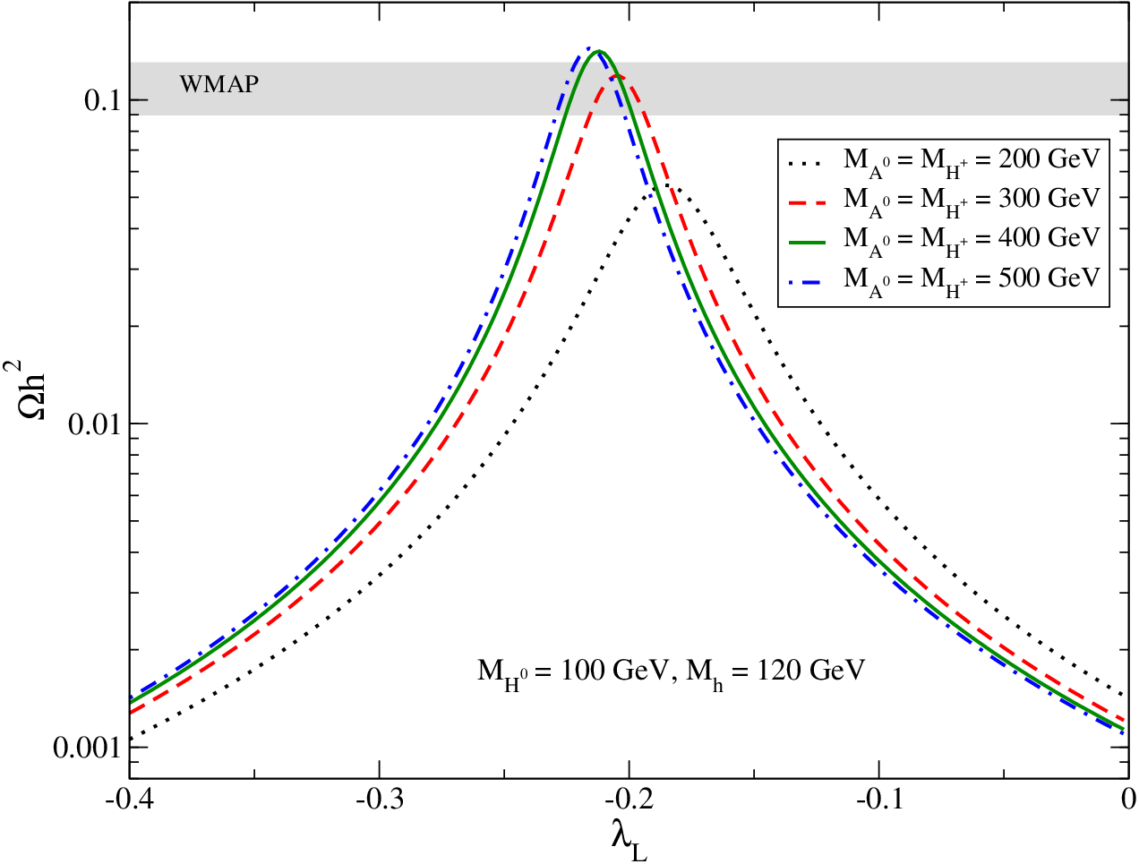
Figure 3 shows the relic density as a function of $\lambda_{L}$ for $M_{H^{0}}=100$ GeV, $M_{h}=120$ GeV and different values of $M_{A^{0}}$ and $M_{H^{\pm}}$. For simplicity we consider models with $M_{A^{0}}=M_{H^{\pm}}$ and we let them vary between $200~\mathrm{GeV}$ and $500~\mathrm{GeV}$. The horizontal band shows the region compatible with the observed dark matter density, $0.09<\Omega h^{2}<0.13$. The effect of cancellations on the relic density is apparent in this figure. They increase $\Omega h^{2}$ significantly as $\lambda_{L}$ approaches about $-0.2$, where the relic density reaches its maximum value. This value depends slightly on the value of $M_{A^{0}}=M_{H^{\pm}}$ but is in any case close to $0.1$. Far from this maximum, say for $\lambda_{L}=-0.4$ or $\lambda_{L}=0$, the relic density is two orders of magnitude smaller. From this figure we also learn that cancellations are necessary but not sufficient to ensure a relic density compatible with the observations. In addition, the mass of the charged scalar (and of the CP-odd scalar) should be large enough to suppress the $H^{\pm}$ (and $A^{0}$) mediated contributions. If, for instance, $M_{H^{\pm}}\lesssim 200~\mathrm{GeV}$ cancellations are still present but the relic density is always below the observed range. For the other values of $M_{H^{\pm}}$ we consider, $300,400,500~\mathrm{GeV}$, it is always possible to satisfy the dark matter constraint for a certain range of $\lambda_{L}$. And the allowed values of $\lambda_{L}$ depend only slightly on the precise value of $M_{H^{\pm}}=M_{A^{0}}$. This first example demonstrates that in the inert doublet model it is indeed possible to satisfy the relic density constraint for $M_{H^{0}}\gtrsim M_{W}$.

The dependence of the relic density on $M_{H^{0}}$ and $M_{h}$ is shown in figure 4. They both display the relic density as a function of $\lambda_{L}$ for $M_{A^{0}}=M_{H^{\pm}}=400~\mathrm{GeV}$. In (a), $M_{H^{0}}$ was set to $100~\mathrm{GeV}$ and four different values of $M_{h}$ ($120,130,140,150~\mathrm{GeV}$) were considered. As before, the horizontal band shows the region compatible with the observed dark matter density. The effect of cancellations are evident: they allow to satisfy the dark matter bound for $\lambda_{L}$ approximately between $-0.15$ (for $M_{h}=150~\mathrm{GeV}$) and $-0.22$ (for $M_{h}=120~\mathrm{GeV}$). As expected from equation (20), the value of $\lambda_{L}$ that gives the maximum relic density moves toward less negative values as $M_{h}$ is increased. Because the Higgs-mediated contribution to dark matter annihilation is proportional to $\lambda_{L}$, the Higgs-dependence of the relic density disappears for $\lambda_{L}=0$, as observed in the figure. At that point, the relic density is driven by the direct annihilation into gauge bosons (figure 1,(a)) resulting in $\Omega h^{2}\sim 10^{-3}$. We can conclude from this figure that for $M_{H^{0}}=100~\mathrm{GeV}$ and $M_{A^{0}}=M_{H^{\pm}}=400~\mathrm{GeV}$ there is a significant range of Higgs masses for which the relic density can be consistent with the observations.

In figure 4 (b) $M_{h}$ was set to $130~\mathrm{GeV}$ and four different values of $M_{H^{0}}$ ($95,100,105,110~\mathrm{GeV}$) were considered. We see that the position of the peak moves toward more negative values of $\lambda_{L}$ as $M_{H^{0}}$ is increased, in agreement with the results found previously. To obtain the observed relic density, values of $\lambda_{L}$ approximately between $-0.15$ (for $M_{H^{0}}=95~\mathrm{GeV}$) and $-0.27$ (for $M_{H^{0}}=110~\mathrm{GeV}$) are required. These figures illustrate that the new viable region occupies a non-negligible volume in the parameter space of the inert doublet model, spanning a significant range in $M_{H^{0}}$, $\lambda_{L}$, $M_{h}$, $M_{A^{0}}$ and $M_{H^{\pm}}$.

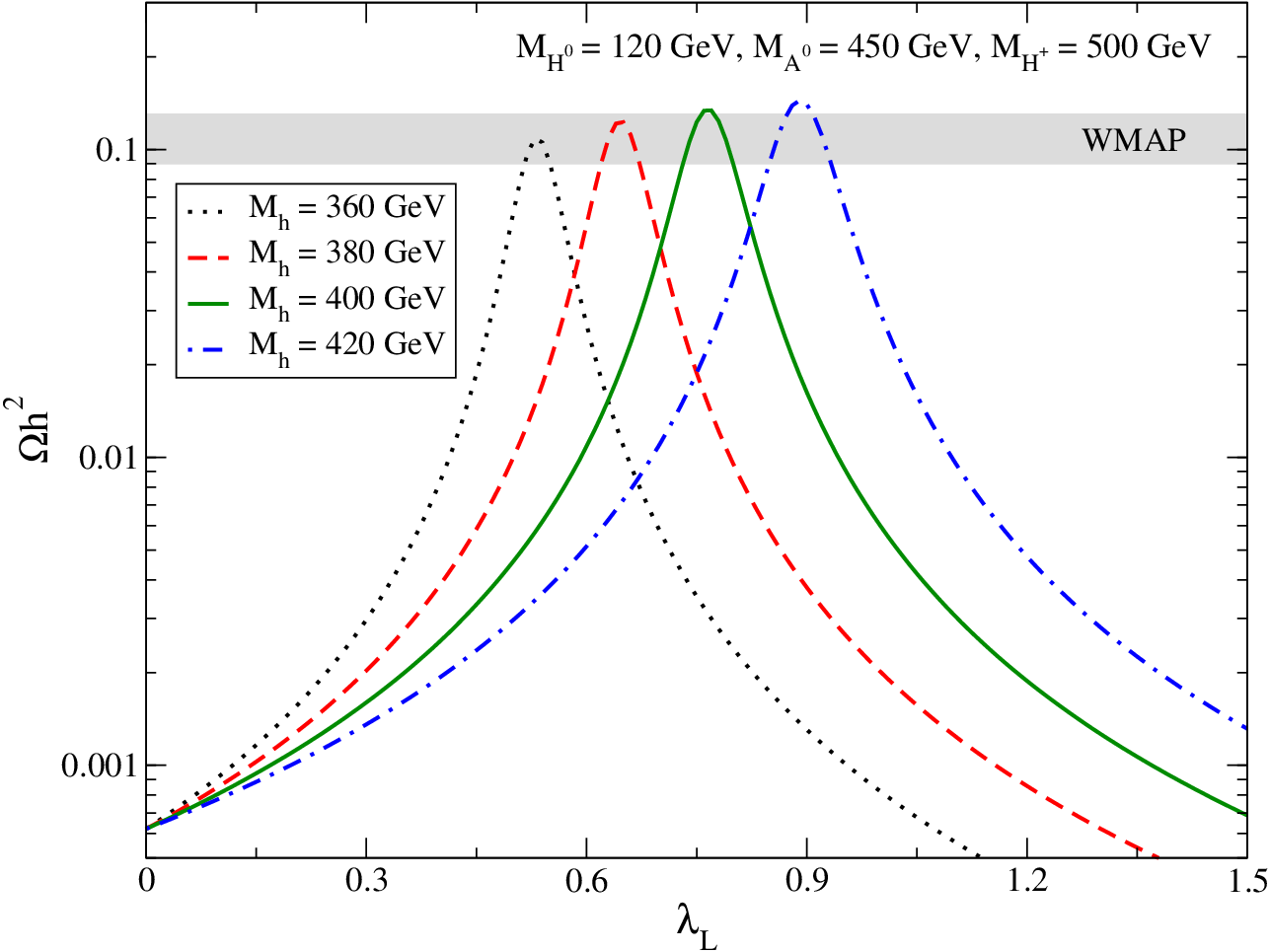
So far we have illustrated the effect of cancellations on the relic density only for the light Higgs regime, $M_{h}\lesssim 200~\mathrm{GeV}$. A remarkable feature of the inert doublet model is that it allows for a much heavier Higgs without contradicting electroweak precision data. As we will see, cancellations leading to viable models with $M_{H^{0}}\gtrsim M_{W}$ can also take place in the heavy Higgs regime of the model, that is for $M_{h}>200~\mathrm{GeV}$.

Figure 5 is analogous to figure 4 but for a heavy Higgs boson, $M_{h}\sim 400~\mathrm{GeV}$. In both panels $M_{H^{\pm}}$ was set to $500~\mathrm{GeV}$ and $M_{A^{0}}$ to $450~\mathrm{GeV}$ (they must now give a positive contribution to $\Delta T$). In (a) the relic density is shown as a function of $\lambda_{L}$ for $M_{H^{0}}=120~\mathrm{GeV}$ and four different values of $M_{h}$: $360,380,400,420~\mathrm{GeV}$. First of all, notice that in this case cancellations occur for positive rather than negative values of $\lambda_{L}$. As expected from the cancellation condition, the position of the peak moves toward larger values of $\lambda_{L}$ as $M_{h}$ is increased. The values of $\lambda_{L}$ that give the correct relic density are between $0.5$ (for $M_{h}=360~\mathrm{GeV}$) and about $0.9$ (for $M_{h}=420~\mathrm{GeV}$). For $\lambda_{L}=0$, $\Omega h^{2}$ becomes independent of $M_{h}$, with a value of about $6\times 10^{-4}$. In (b) the relic density is shown as a function of $\lambda_{L}$ for $M_{h}=400~\mathrm{GeV}$ and four different values of $M_{H^{0}}$: $100,110,120,130~\mathrm{GeV}$. The viable region corresponds in this case to $\lambda_{L}$ between $0.7$ (for $M_{H^{0}}=130~\mathrm{GeV}$) and $1.0$ (for $M_{H^{0}}=100~\mathrm{GeV}$). We observe that the maximum value of $\Omega h^{2}$ increases as $M_{H^{0}}$ is decreased. In fact, if $M_{H^{0}}=130~\mathrm{GeV}$ the maximum relic density is as large as the WMAP lower limit. So, it is not possible to satisfy the relic density constraint (keeping the other parameters fixed) for $M_{H^{0}}>130~\mathrm{GeV}$. But if $M_{H^{0}}=100~\mathrm{GeV}$ the relic density can be larger than the WMAP upper limit, reaching about $0.23$. As a result, it is easier to satisfy the relic density constraint with a lighter inert Higgs.

As we have seen in the previous figures, cancellations between the different diagrams that contribute to dark matter annihilation into gauge bosons indeed allow to satisfy the relic density constraint for inert Higgs masses above $M_{W}$ (and below $m_{t}$). In other words, there certainly exist regions in the viable parameter space of the inert doublet model that had not been considered before. What we are lacking at this point is a more complete characterization of this new viable region. We would like to know, for instance, what is the largest dark matter mass ($M_{H^{0}}$) that is allowed, what are the typical values of $\lambda_{L}$, $M_{h}$, $M_{H^{\pm}}$ and $M_{A^{0}}$, or what is the most promising strategy to detect the inert Higgs along this region. In the next sections we will address precisely these issues.

The inert doublet model contains $5$ free parameters that can be taken to be $M_{H^{0}}$, $M_{H^{\pm}}$, $M_{A^{0}}$, $\lambda_{L}$, and $M_{h}$. We allow these parameters to vary within the following ranges:

MCMC tecniques allow us to scan freely and efficiently over these $5$ parameters. Let us emphasize that these techniques have already been successfully used to scan and analyze the viable parameter space of other models of dark matter, see [38, 39]. Here we closely follow the procedure outlined in [38].

After scanning the above parameter space, we get a large sample of viable models, satisfying all the experimental and theoretical bounds and the relic density constraint. For our analysis we generated about 40000 such models within the new viable region. In the remaining part of the paper, we will work exclusively with this sample of models, analyzing its main features and studying its implications.

To facilitate the analysis and visualization of the 5-dimensional region where the viable models are located, we will project it onto different two-dimensional planes. Figure 6, for instance, shows the new viable region of the inert doublet model in the plane ($M_{H^{0}}$,$\lambda_{L}$). To generate this kind of figures, we created a suitable grid in the two variables ($M_{H^{0}}$ and $\lambda_{L}$ in this case) and we place a point at a given value of them if there is at least one viable model in our sample with such coordinates. Sometimes we also differentiate (using symbols and colours) various ranges for other important parameters (the Higgs mass in figure 6) that may provide additional information. Notice in figure 6 that the value of $M_{H^{0}}$ over the new region extends from $M_{W}$ up to about $160~\mathrm{GeV}$. We argued in section 4 that $M_{H^{0}}$ had to be smaller than $m_{t}=171.4~\mathrm{GeV}$ but at that point we did not know how close to $m_{t}$ it could get. In $\lambda_{L}$, the range of possible values extends from $-0.5$ to about $3.0$. A sharp contrast is observed between the models with $\lambda_{L}<0$ and those with $\lambda_{L}>0$. In the former case ($\lambda_{L}<0$), the maximum value of $M_{H^{0}}$ is about $130~\mathrm{GeV}$ and the Higgs boson is necessarily light, $M_{h}<200~\mathrm{GeV}$, as cancellations occur for $M_{H^{0}}>M_{h}/2$. In the latter case ($\lambda_{L}>0$), the maximum value of $M_{H^{0}}$ can be larger, strongly depending on the range of Higgs masses. Thus, for $200~\mathrm{GeV}<M_{h}<300~\mathrm{GeV}$ the maximum $M_{H^{0}}$ is only about $110~\mathrm{GeV}$ whereas it can reach almost $160~\mathrm{GeV}$ for the largest Higgs masses, $M_{h}>500~\mathrm{GeV}$. It is also apparent from the figure, that for $\lambda_{L}>0$ the larger the Higgs mass the larger $\lambda_{L}$ must be. Given that cancellations are needed to obtain the correct relic density, it is not surprising that no viable models are found with $\lambda_{L}$ close to zero, as in that region the Higgs-mediated diagram becomes negligible. Finally, the dashed line shows the contour $\mu_{2}^{2}=0$. From the figure we see that viable points with $\mu_{2}^{2}>0$ feature $\lambda_{L}<0$ and viceversa.

The dependence of the new viable region on $M_{H^{\pm}}$ and $M_{A^{0}}$ is illustrated in figure 7. Panel (a) shows the projection on the plane ($M_{H^{0}}$, $M_{H^{\pm}}$) for different ranges of $M_{A^{0}}$. The trend is clear: the heavier the dark matter particle the larger $M_{H^{\pm}}$ must be. If $M_{H^{0}}<100~\mathrm{GeV}$, $M_{H^{\pm}}$ can take values within a wide range, but as $M_{H^{0}}$ increases, higher and higher values of $M_{H^{\pm}}$ are required. If, for instance, $M_{H^{0}}>130~\mathrm{GeV}$, $M_{H^{\pm}}$ should be larger than about $400~\mathrm{GeV}$. And the viable models with the highest dark matter masses ($M_{H^{0}}>150~\mathrm{GeV}$) all feature a heavy $H^{\pm}$ (and a heavy $A^{0}$), $M_{H^{\pm}}>500~\mathrm{GeV}$. It is also observed in the figure that there is a correlation between the values of $M_{H^{\pm}}$ and $M_{A^{0}}$. Large values of $M_{H^{\pm}}$ are associated with large values of $M_{A^{0}}$. This correlation is illustrated in more detail in panel (b) of the same figure, which shows the viable region in the plane ($M_{A^{0}}$,$M_{H^{\pm}}$) for different ranges of the Higgs mass. In this plane, the viable models are concentrated along a band just above the $M_{H^{\pm}}=M_{A^{0}}$ line (the diagonal). In other words, most models feature $M_{H^{\pm}}>M_{A^{0}}$ but their mass splitting is never that large. Let us emphasize that this condition is not enforced by the dark matter constraint but rather by electroweak precision data, see equations (9) and (12). We see then that both $M_{A^{0}}$ and $M_{H^{\pm}}$ can be as large as $650~\mathrm{GeV}$ and that the models with the highest dark matter masses ($M_{H^{0}}\gtrsim 140~\mathrm{GeV}$) require them to be larger than about $500~\mathrm{GeV}$.

In figure 8 we show the new viable region in the plane ($M_{H^{0}}$,$M_{h}$). The Higgs resonance line, $2M_{H^{0}}=M_{h}$, is also shown for illustration. A priori we do not expect to find viable models close to that line, for resonant annihilations would drive the relic density to very small values. Points lying below the Higgs resonance line correspond to models with $2M_{H^{0}}>M_{h}$ and they all feature $\lambda_{L}<0$. From the figure we see that such points extend up to about $130~\mathrm{GeV}$ in $M_{H^{0}}$ and about $160~\mathrm{GeV}$ in $M_{h}$. They correspond, therefore, to what we call the light Higgs regime. Points above the Higgs resonance line ($2M_{H^{0}}<M_{h}$), in constrast, all feature a positive value of $\lambda_{L}$. It can be observed that they include dark matter masses as high as $160~\mathrm{GeV}$ and Higgs bosons heavier than $200~\mathrm{GeV}$ and extending up to $600~\mathrm{GeV}$. Hence, they lie within the heavy Higgs regime. Finally it is worth mentioning that no viable models are found for Higgs masses approximately between $160~\mathrm{GeV}$ and $200~\mathrm{GeV}$.

We have in this way determined the position of the new viable region in the 5-dimensional space formed by $M_{H^{0}}$, $M_{A^{0}}$, $M_{H^{\pm}}$, $\lambda_{L}$ and $M_{h}$. It is also useful to understand its position in the space of $\lambda$ parameters, which consists of $\lambda_{3}$, $\lambda_{4}$ and $\lambda_{5}$. The reason is that some constraints, such as the perturbativity and the vacuum stability bounds, are applied directly to these couplings, not to scalar masses or to $\lambda_{L}$. Since many models feature a rather heavy $H^{\pm}$ and $\mu_{2}^{2}$ negative (equivalently $\lambda_{L}$ positive), we expect that a larger value of $\lambda_{3}$ will be required –see equation (2). That is what we observed in figure 9. It displays the new viable region in the plane ($M_{H^{0}}$,$\lambda_{3}$) for different ranges of $M_{h}$. We see that $\lambda_{3}$ can indeed be large, with some models lying right at the perturbativity limit, $\lambda_{3}=4\pi$ (dotted line). In the figure we observe that the models with the largest dark matter masses ($M_{H^{0}}\gtrsim 140~\mathrm{GeV}$), in particular, feature $\lambda_{3}\gtrsim 9$. It must be emphasized, however, that $\lambda_{3}$ is not that large over the entire new viable region. Models with $\lambda_{3}<6$, for instance, extend up to $M_{H^{0}}=120~\mathrm{GeV}$ while those with $\lambda_{3}\lesssim 2$ can reach up to $105~\mathrm{GeV}$. Thus, if one wants to impose a more restrictive perturbativity bound on $\lambda_{3}$, this figure can be used to find out the resulting viable range of $M_{H^{0}}$.

Figure 10 shows the new viable regions in the planes ($M_{H^{0}}$,$\lambda_{4}$) and ($M_{H^{0}}$,$\lambda_{5}$). $\lambda_{4}$ turns out to be negative in most models and reaches at most $|\lambda_{4}|=7$, significantly below the perturbativity limit (not shown). The possible values of $\lambda_{4}$ move toward lower values as $M_{H^{0}}$ is increased. Hence, for $M_{H^{0}}=100~\mathrm{GeV}$ $\lambda_{4}\in\left(-1,-7\right)$ whereas for $M_{H^{0}}=130~\mathrm{GeV}$ $\lambda_{4}\in\left(-3,-7\right)$. Notice also that $\lambda_{4}\sim-5$ for the models with the largest values of $M_{H^{0}}$. $\lambda_{5}$, which determines the mass splitting between $H^{0}$ and $A^{0}$, is by definition negative ($M_{A^{0}}>M_{H^{0}}$). We see, in panel (b), that its absolute value is never larger than $7$ and only rarely exceeds $5$, placing it comfortably within the perturbative regime. As with $\lambda_{4}$, the allowed values of $\lambda_{5}$ tend to move toward lower values (higher $|\lambda_{5}|$) as $M_{H^{0}}$ is increased. For the models with the highest dark matter masses, $\lambda_{5}$ is about $-4.0$. Consequently, a more restrictive pertubativity bound on $\lambda_{4}$ and $\lambda_{5}$, say $\lambda_{4,5}<5$, could be imposed without affecting the viable range of $M_{H^{0}}$.

We thus conclude this subsection regarding the projections of the viable region onto different two-dimensional planes. Before addressing the implications of the new viable region for the direct and the indirect detection of inert Higgs dark matter, we will discuss the issue of the fine-tuning required to obtain the correct relic density within this new viable region. Is it large, moderate or small? How does it compare against the fine-tuning found in other models of dark matter?

Given that in it cancellations are necessary to obtain the right relic density, one may think that this new viable region of the inert doublet model is disfavoured by fine-tuning arguments. Here, we quantify the fine-tuning of the viable models and show that that is not really the case. Many of them feature low to moderate fine-tuning and none of them has a very large one.

The issue of the fine-tuning required to satisfy the dark matter constraint is not new. In [40], where this fine-tuning was first quantified, it was proposed to use as a fine-tuning parameter the logarithmic sensitivity of the relic density to variations in the input parameters of the model. If $a_{i}$ ($i=1,...,n$) are free parameters of a given dark matter model, the fine-tuning parameter (of the relic density) with respect to $a_{i}$, $\Delta_{\Omega h^{2},a_{i}}$ is given by

And the total fine-tuning, $\Delta_{\Omega h^{2},\mathrm{total}}$, is obtained by summing in quadrature the contributions of the different parameters of the model. Thus, in the inert doublet model we have that

Hence, the fine-tuning parameter is large if a small variation in the parameters of the models leads to a large modification of the relic density. If, for instance, $\Delta_{\Omega h^{2},\mathrm{total}}\lesssim 10$, a measurement of the parameters of the model at the $10\%$ level will enable to compute $\Omega h^{2}$ to within a factor $\mathcal{O}(2)$. As a rule of thumb, one can say that the fine-tuning is small if $\Delta_{\Omega h^{2},\mathrm{total}}\lesssim 10$, moderate for $10<\Delta_{\Omega h^{2},\mathrm{total}}\lesssim 100$ and large if $\Delta_{\Omega h^{2},\mathrm{total}}>100$.

Figure 11 shows the fine-tuning parameter as a function of $M_{H^{0}}$ along the new viable region of the inert doublet model. $\Delta_{\Omega h^{2},\mathrm{total}}$ is typically smaller than $30$, with plenty of models featuring $\Delta_{\Omega h^{2},\mathrm{total}}<10$ over the entire range of $M_{H^{0}}$ and no models with a fine-tuning parameter larger than $40$. In particular, notice that there is no correlation between $\Delta_{\Omega h^{2},\mathrm{total}}$ and $M_{H^{0}}$. Low fine-tuning models, $\Delta_{\Omega h^{2},\mathrm{total}}\lesssim 10$, exist for $M_{H^{0}}$ just slightly above $M_{W}$ as well as for $M_{H^{0}}>140~\mathrm{GeV}$. And the same holds for moderate fine-tuning models, $\Delta_{\Omega h^{2},\mathrm{total}}\gtrsim 20$.

These results can be compared with those obtained in previous works for one of the most studied models of dark matter, the Constrained Minimal Supersymmetric Standard Model (CMSSM or mSUGRA). It turns out that the viable regions of the CMSSM tend to be highly fine-tuned, with some regions, such as the focus-point and the funnel region, featuring a $\Delta_{\Omega h^{2},\mathrm{total}}$ greater than $100$ [40, 41]. In contrast, in the new viable region of the inert doublet model we are studying, the fine-tuning parameter is never that high.

The inert doublet model can be tested at colliders via the production and decay of inert particles or through the increase in the decay width of the Higgs boson [13]. Indeed, the decay processes

may enhance the Standard Model Higgs decay width when $M_{h}>2M_{H^{0}}$, with important implications for Higgs searches at Tevatron and at the LHC. For the dark matter mass range we are studying, this increase is mainly due to the $H^{0}H^{0}$ final state and it takes place only when $\lambda_{L}>0$ and $M_{h}>200$ GeV, see figure 6. As a consequence, the Higgs decay width considered in the recent summary of Higgs searches at Tevatron below 200 GeV [42] is left untouched by the inert scalars for $M_{H^{0}}>M_{W}$. The LHC, on the other hand, is expected to perform direct measurements of the Higgs decay width with a precision of about 6% [43] for $300~\mathrm{GeV}<M_{h}<700~\mathrm{GeV}$.

Figure 12 shows the Higgs branching ratio into $H^{0}H^{0}$ as a function of the Higgs mass for our sample of viable models. It lies approximately between $5\%$ and $60\%$. In this figure, different ranges of $M_{H^{0}}$ are distinguished. For models with $M_{H^{0}}>140~\mathrm{GeV}$, BR($h\to H^{0}H^{0}$) is observed to be about $10\%$ or less. Branching ratios greater than $20\%$ or so can also be found but only for models with the smallest dark matter masses, $M_{H^{0}}\lesssim 100~\mathrm{GeV}$. In such case, the inert Higgs could be within the reach of LHC via measurements of the Higgs decay width.

The indirect detection signatures of dark matter are determined, on the particle physics side, by the present annihilation rate and by the annihilation branching ratios. Figure 13 shows the present dark matter annihilation rate, $\sigma\mathrm{v}$, as a function of $M_{H^{0}}$ along the new viable region ($\mathrm{v}$ is taken to be $10^{-3}$). We see that most points are confined within a small interval between $0.5\times 10^{-26}\mathrm{cm^{3}/s}$ and $4\times 10^{-26}\mathrm{cm^{3}/s}$. In other words, the present annihilation rate is always close to the typical value for a thermal relic, $\langle\sigma\mathrm{v}\rangle\sim 3\times 10^{-26}\mathrm{cm^{3}/s}$. This outcome is a consequence of the fact that the annihilation of inert Higgs dark matter is dominated by its s-wave component, so $\sigma\mathrm{v}$ remains unchanged between the early Universe and the present time. Besides, coannihilations, with $A^{0}$ or $H^{\pm}$, play no important role in the region we are considering, as they would drive the relic density to even smaller values.

In the new viable region, the inert Higgs annihilates mainly into $b\bar{b}$, $W^{+}W^{-}$ and $Z^{0}Z^{0}$ (the $hh$ and $t\bar{t}$ final states are kinematically forbidden). Figure 14 shows the annihilation branching ratio (BR) into these three final states as a function of $M_{H^{0}}$. We see, in the left panel, that the maximum value of BR($H^{0}H^{0}\to b\bar{b}$) decreases with $M_{H^{0}}$, going from about $0.85$ for $M_{H^{0}}\sim 80~\mathrm{GeV}$ to about $0.2$ for $M_{H^{0}}\sim 140~\mathrm{GeV}$. The minimum value of BR($H^{0}H^{0}\to b\bar{b}$), on the other hand, tends to remain constant at about $0.15$. In particular, the $b\bar{b}$ final state is never negligible within the new viable region. The center panel shows the branching ratio into $W^{+}W^{-}$. As $M_{H^{0}}$ crosses the $Z^{0}$ threshold, the annihilation into $Z^{0}Z^{0}$ start playing a significant role and the branching into $W^{+}W^{-}$ is therefore reduced. It is also observed in figure 14 that the range of variation of BR($H^{0}H^{0}\to W^{+}W^{-}$) shrinks as $M_{H^{0}}$ increases. For $M_{H^{0}}>120~\mathrm{GeV}$ BR($H^{0}H^{0}\to W^{+}W^{-}$) lies approximately between $0.3$ and $0.5$. Finally, the right panel shows BR($H^{0}H^{0}\to Z^{0}Z^{0}$). It never exceeds $40\%$, reaching values between $0.25$ and $0.35$ for $M_{H^{0}}>120~\mathrm{GeV}$, and lower values for smaller $M_{H^{0}}$. Comparing the three panels we can deduce that $b\bar{b}$, $W^{+}W^{-}$ and $Z^{0}Z^{0}$ are indeed the dominant annihilation channels, as their combined branching is always close to $100\%$. The remaining annihilation channels, into light fermions, typically account for less than $10\%$ of the annihilations.

The present annihilation rate and the branching ratios that we have calculated determine the indirect detection signatures of inert Higgs dark matter. To illustrate the prospects for the indirect detection of dark matter along this new viable region, we compute the expected gamma ray flux from the annihilation of inert Higgs particles and compare it with present data from FERMI.

The gamma ray flux from dark matter annihilations originating in a region $\Delta\Omega$ of the sky can be written as

where $r_{\odot}=8.5\mathrm{~kpc}$ is the distance from the Sun to the Galactic Center, $\rho_{\odot}=0.39~\mathrm{GeV}/\mathrm{cm^{3}}$ is the local density of dark matter [44], $dN/dE$ is the photon spectrum, and $\bar{J}\Delta\Omega$ is given by

For the galactic distribution of dark matter we consider a NFW profile [45],

where $r_{s}=20\,$kpc and $\rho_{s}=0.34\,\mathrm{GeV}/\mathrm{cm^{3}}$. For definiteness we consider the observation region $10^{\circ}<|b|<20^{\circ}$, for which there is available data from FERMI – see [46] and the supplementary online material. The photon spectrum from dark matter annihilations, $dN/dE$, depends on the annihilation branching ratios and has been obtained using micrOMEGAs.

Figure 15 shows the differential gamma ray flux at $1~\mathrm{GeV}$ (left panel) and at $10~\mathrm{GeV}$ (right panel) for our sample of models. For $E_{\gamma}=10~\mathrm{GeV}$, it lies approximately between $5.0\times 10^{-6}$ and $2.5\times 10^{-5}~\mathrm{MeV/(cm^{2}\,s\,sr)}$, and at slightly smaller values (particularly at large masses) for $1~\mathrm{GeV}$. Unfortunately, these fluxes are much smaller than those measured by FERMI [46], which are consistent with the predictions of cosmic ray models. It is thus not possible to obtain any constraints from this data.

Let us stress that this somewhat disappointing result is consistent with previous analysis of FERMI data, see e.g. [47]. In them, it had been found that present data from FERMI can be used to rule out dark matter annihilation cross sections exceeding $10^{-23}$ or $10^{-24}~\mathrm{cm^{3}/s}$ (depending on the dark matter mass and annihilation final state). Such cross sections are much larger than those expected in typical models of dark matter and, in particular, than those we have found along the new viable region of the inert doublet model.

Dark matter can also be detected via elastic scattering with terrestrial detectors, the so-called direct detection method. From a particle physics point of view, the quantity that determines the direct detection rate of a dark matter particle is the dark matter-nucleon scattering cross section. In the inert Higgs model, the $H^{0}N$ scattering process relevant for direct detection is Higgs-mediated, with a cross section, $\sigma_{H^{0}N}$, given by

where $f\sim 0.3$ is a form factor and $m_{r}$ is the reduced mass of the system. Thus, it is proportional to $\lambda_{L}^{2}$. Given the rather large values of $\lambda_{L}$ we found, see figure 6, we foresee that $\sigma_{H^{0}N}$ will be significant over the entire new viable region. Figure 16 shows the spin-independent dark matter-nucleon cross section, $\sigma_{H^{0}N}$, as a function of $M_{H^{0}}$ for our sample of models. $\sigma_{H^{0}N}$ lies in a narrow range between $3\times 10^{-7}$ and $10^{-8}$ Pb. To ease the comparison with present experimental data, the bound from the CDMS experiment [37] is also shown (as a solid line) as well as the expected sensitivity of Xenon100 (dotted line) [48]. Points lying above the CDMS line are not consistent with present bounds whereas points above the Xenon100 line are within the reach of that experiment. As observed in the figure, a non-negligible fraction of the new viable region is ruled out by direct detection constraints. In particular, most models with $M_{h}<200~\mathrm{GeV}$ (though not all of them) have a direct detection cross section exceeding the CDMS bound. No range of $M_{H^{0}}$ is excluded, however. The good news is that all these viable models feature cross sections close to current bounds. They are all well within the sensitivity of Xenon100. Clearly, direct detection is a promising way of probing this new viable region of the inert doublet model.