An analysis of the Brown-Biefeld effect
Abstract
When a high voltage is applied on an asymmetric capacitor,
it experiences a force acting toward its thinner electrode. This
effect is called Brown-Biefeld effect (BB), after its discoverers
Thomas-Townsend Brown and Paul-Alfred Biefeld. Many theories have been
proposed to explain this effect, and many speculations can be found on
the net suggesting the effect is an antigravitation or a space warp
effect. However, in the recent years, more an more researchers
attribute the BB effect to a unicharge ion wind. This work calculates
the levitation force due to ion wind and presents experimental results
which confirm the theoretical results.
Keywords:
brown-biefeld, lifters, electrostatics, corona, ion drift, Deutsch assumptionPACS: 41.20.Cv, 52.30.-q, 41.20.-q
1. INTRODUCTION
The Brown-Biefeld (BB) effect has been discovered in 1920 by Thomas Townsend Brown and Paul Alfred Biefeld during their experiments with Coolidge X-ray tube. They observed a thrust acting toward the thin electrode. Thomas Townsend Brown made an extensive research on this effect and wrote several patents [1, 2, 3].
There is a site dedicated to the BB effect [4] and a site dedicated to experiments of this effect [5], but very few theoretical works have been written on the subject. Some of those tried to explain the effect by electro-gravitation [6, 7, 8] or thermodynamics [9].
However, in the recent years more and more sources [10, 11, 12, 13] attribute the effect to corona ionic air propulsion. In [13] a lot of experiments are described, and the thrust force is described by approximate formulas based on ion propulsion, and in [11] a full calculation of the thrust, based on the jet of the corona ion wind is performed. The calculations in [11] were very accurate, but seemed to require a substantial amount of computing power.
In this work we also calculate the force due to ionic air propulsion, but we adopt a different approach, based on the Deutsch assumption [14], which has been extensively used in the unipolar charge flow literature [15, 16, 17, 18, 19, 22, 23, 24], but also criticized (see J. E. Jones et al. [20] and A. Bouziane et al. [21]), by showing big differences in magnitude and direction between the exact electric fields and the ones obtained with the Deutsch assumption. However our goal is to calculate the thrust force and for this purpose the Deutsch assumption proves useful.
The Deutsch assumption states that the equipotential surfaces of the Laplacian problem are equipotential also for the Poissonian problem, only with different values of potential. Of course under this assumption, the electric field lines of the Laplacian and Poissonian problems are in the same direction at any location.
As we shall see, the calculations based on Deutsch assumption [14], within the Warburg region [26, 27] result in formulas which fit very well the experiment.
In Section 2 we explain the operation principle and the configuration which has been analyzed. We also present the equations that have to be solved.
In Section 3 we present the basics of the Deutsch assumption. Sigmond [18] made a profound analysis on the subject, and summarized the work of many researchers concerning the use of the Deutsch assumption. We will summarize those findings, and bring some highlights on this issue.
In Section 4 we solve the Laplacian problem and calculate the capacitance. Those results are new, because as far as we know this Laplacian configuration has not been solved yet. Also, this Laplacian solution is needed for the Poissonian problem when Deutsch assumption is used.
In Section 5 we solve the Poissonian problem using the Laplacian solution and Deutsch assumption and display the calculated force and current.
In Section 6 we describe our experiment and show the obtained results.
In Section 7 we compare the measured and calculated results and express our calculated results by approximate formulas.
The work is ended with some concluding remarks.
2. THE OPERATION PRINCIPLE AND THE CONFIGURATION
The picture of the lifter on which we did our experiments is shown in Figure 1. The lifter is based on a thin anode wire at positive high voltage, over a grounded flat cathode. As follows from the explanation below, for best propulsion, the flat electrode must be vertical. We made some experiments with negative corona and the thrust is considerably lower for negative corona than for positive corona, fact which is confirmed by Blazelabs [13]. Hence we start the explanation for positive corona.

The working principle is as follows: when a high enough positive voltage is supplied, pairs of positive ion and electron (which are always randomly created by incident photons) are accelerated: the positive ion toward the cathode and the electron toward the anode. Some of those pairs recombine emitting a photon which by the photoelectric effect on a neutral atom, ionizes it, creating the electron avalanche. High energy electrons hitting neutral atoms, ionize them, contributing to the avalanche. This process arrives to a steady state consisting in a corona region around the anode (in which the ionization process happens) and in which there are positive ions and high speed electrons. Hence this region is neutral and typically narrow and outside it there is a unicharge positive ion drift moving toward the cathode. The positive ions transfer most of their momentum to neutral molecules and while the positive ions “feel” the force of the electric field and hence move toward the cathode (according to the positive ion mobility coefficient) the neutral molecules keep the inertia of the momentum they received. If the flat cathode were horizontal (and infinite), the jet of neutral molecules would hit the cathode and hence the forces on the anode and cathode would have been equal and opposite, hence no net thrust.
However, the cathode being vertical, and given the fact that the ions transfer most of their momentum to neutral molecules, those do not hit the cathode, but form an air jet downstairs, and by momentum conservation the lifter senses a net force upwards. Hence, the thrust force is calculated as the total force on the space charge.
Also we treat the whole region as unicharge, and neglect the corona thickness, which is small for the case of positive corona [11, 13, 28].
About negative corona: negative corona starts like the positive corona by randomly created pairs of positive ions and electrons, only here the positive ions are accelerated toward the negative thin electrode (called here cathode) and the electrons are accelerated toward the flat electrode (called now anode). Also for negative corona some pairs recombine, emitting a photon, but this time the photoelectric effect created by it is on the thin wire surface, which being negative, easily releases electrons, creating the electron avalanche. Also electrons hit neutral atoms and ionize them, but because the electrons move outward the negative thin electrode, this happens at lower velocities than for positive corona, hence this part of the process is less dominant. Hence, the photoelectric effect on the thin wire surface being dominant, the negative corona is very sensitive to the ability of the thin wire to emit electrons. If the thin wire surface has irregularities only some parts of it emit electrons, creating tufts (see Peek [28], Fig. 77). Also for a limiting voltage, for which the thin wire surface is not able to steadily emit electrons, the process may be bursty. This happens because the positive ions attracted to the thin wire lower the strength of the electric field near it, and this field is restored only after the emitted electrons enter the flat positive conductor and arrive through the power source to the thin negative wire. If the process arrives to a steady state, the negative corona has two layers: the inner layer called ionization layer which consists of positive ions and out flowing electrons emitted by the thin wire, the outer layer in which electrons flow out bouncing into neutral atoms and combine in negative ions. Outside those layers there is a unicharge flow of negative ions and electrons (see [25], Fig. 1). We suppose the main reasons for the levitating force being smaller with negative corona are the tufts (reflecting a nonuniform ability of the thin wire to emit electrons) and burstiness which may persist also after corona builds up. We will not further deal with negative corona and all the results obtained in this paper are valid for positive corona only.
Now the shape of the lifter must not necessarily be triangular, it may be rectangular or any other shape. Neglecting edge effects, the operation is described by a thin anode wire, over a vertical conducting plane. Hence we deal with a two dimensional problem described in Figure 2.

Our lifter has the following dimensions: , and (see Figure 2). Each side of the triangle is , hence if we calculate the thrust force per unit length, we have to multiply by the perimeter of to find the total force.
As long as the potential difference is below the corona inception voltage [28], there is no space charge, hence we have a Laplacian problem, defined by
| (1) |
where the index “L” denotes the Laplacian solution. The boundary conditions are on the anode wire surface and on the cathode wire surface, where is the applied voltage. The electric field is .
In presence of space charge, different kinds of ions have different mobilities, defining the velocity of each ion as its mobility times the electric field. However, we use the average mobility [13, 17, 20] for positive air ions, known to be . Diffusion can usually be neglected [29, 30], hence the unipolar non diffusive drift of ions is described by
| (2) |
where is the space charge per unit of volume and is not the Laplacian field, but the Poissonian field, influenced by the space charge itself via Gauss law:
| (3) |
Being a stationary problem, the current conservation condition must hold. So the Poissonian problem may be formulated by: or
| (4) |
Clearly, this equation contains the 3rd derivative, hence one needs an additional boundary condition, and what is usually assumed is Kaptzov hypothesis [31].
Physically Kaptzov hypothesis means that once the potential difference has been raised sufficiently for the corona to start, the electric field near the corona conductor remains constant and equals the inception value, even when further raising the potential difference.
Our goal is to calculate the thrust force, i.e. the component of the total force on the space charge , where is the component of , and the integral is on the whole free space. Using eq. (2), the total thrust force may be expressed as
| (5) |
and for this goal we need a full solution of eq. (4). Felici [29] analyzed equation (4) and gave some particular solutions, and Feng [32] calculated an exact solution of eq. (4) for concentric cylinders.
As mentioned before, eq. (4) is easier to
solve by using the Deutsch assumption [14] and this item
is discussed in the following section.
3. ANALYSIS OF THE DEUTSCH ASSUMPTION
The Deutsch [14] assumption (DA) states that the equipotential surfaces of the Laplacian problem, defined by eq. (1) are equipotential also for the Poissonian problem, defined by eq. (4), only with different values of potential. This assumption is not valid in general, hence its usage violates some laws of physics. Sigmond [18] studied the consequences of using DA, and showed that there are two general approaches in using DA. One approach called T-type, keeps , but violates current conservation. The other approach called L-type, satisfies the current conservation but violates the orthogonality between flux lines and potential surfaces (i.e. results in ).
For more details, the reader is referred to [18], formulas (13)-(39), but for convenience we show here the main highlights of the issue. Dealing with a two dimensional problem we shall use orthogonal coordinates describing the field direction and equipotential surfaces, respectively (the equivalents of in [18]). Accordingly, the unit vectors will be noted as .
The assumption that the equipotential surfaces of the Laplacian problem remain equipotential in the Poissonian problem implies that the Poissonian field can be expressed as
| (6) |
where is a scalar function. It is crucial for our solution to have a correct current distribution, because from eq. (5) we see that only a correct current can result in a correct force, hence we use the L-type described above. Requiring current conservation and using eq. (2) and (6) we obtain
| (7) |
because . Now pointing in the direction, and being non zero, implies:
| (8) |
which means that must be a function of only:
| (9) |
| (10) |
This method has been carried out by Popkov [22] and he showed that one may obtain the potential difference on each field line as a function of the current density on the collector, and used cross-plot technique to obtain the current density in terms of the applied voltage. Sarma and Janischewskyj [23] followed the same technique as Popkov, but used an iterative procedure to calculate the current density on each field line in terms of the applied voltage. A. Bouziane et al. [24]) used the above methods to evaluate the current density and field profile for several geometries, and found the results in agreement with experiment.
Our goal is to calculate the thrust force in eq. (5), hence we will not follow the above techniques, but rather look for an adequate function . It will be helpful for example if we could choose this function to be constant in some regions of .
Now because we used the L-type, in general, so if we require we end with a contradiction.
As we shall see in the next section, the Laplacian field lines are almost straight in the paraxial region around (see Figure 2). It is therefore of interest to examine what happens in a region where the Laplacian field lines are straight. In such region the unit vector does not change with , so is a function only. Knowing that , results in being a function of only.
We shall see that in this case we may require , because this belongs to the cases described in [18], eqn. (38) and (39), for which the DA holds exactly. So requiring:
| (11) |
results in being in the direction, hence being only a function of . Therefore is also a function of only, and the same is true for .
The outcome is that in eq. (9) which is only a function of must also be only a function of . This is possible only if the function in eq. (10) is a constant.
This is helpful, since we may start our Poissonian calculations (Sect. 5) in the paraxial region with constant, and let it drop to 0 when approaching the Warburg [26, 27] limit region.
This is in accordance with the experimental knowledge that the current drops to 0 outside the Warburg region [34, 35, 36, 37] and also with Ieta [16], who showed that the Laplacian solution reconstructs well the Warburg distribution for a pin to plane geometry. As we shall see, this method results in a calculated thrust force which fits experiment.
So, for using Deutsch assumption in the Poissonian problem, we need the
solution to the Laplacian problem first, and this is done in the next
section.
4. SOLUTION OF THE LAPLACIAN PROBLEM
There are many ways to solve the Laplacian problem (analytic or numeric) and we chose to solve it analytically, by separation of variables in cylindrical coordinates.
The schematic configuration in Figure 2, does not allow to properly define boundary conditions in separate variables in cylindrical coordinates, hence we will make a slight change to this configuration.
Anyhow the configuration in Figure 2 is not accurate, because it does not show the width of the flat cathode. In practice the cathode must have a finite width, and more than that, the curvature radius of the cathode at the location (see Figure 2) must be big enough so that no corona can be formed there [28].
The modified configuration is described in Figure 3.

The flat cathode surface is now defined along , where is a fixed small angle of about (based on the thickness of the cathode in our lifter). This model still includes edges at , but those edges do not exist in the real engine and except of them the model is quite close to reality. At last, we take the cathode length to infinity: the main interaction is between the electrodes and using a finite length would still be solvable analytically, but would be an unnecessary complication.
We define the potential for the region and and the potential for the region and . The boundary conditions are:
| (12) |
where is the applied voltage. Because of the mirror symmetry around the axis, we require
| (13) |
The potential continuity at gives
| (14) |
and the normal field continuity at requires
| (15) |
The potential is on the sides of the big conductor
| (16) |
and must go to at :
| (17) |
We will use the well known solutions for the Laplace equation in cylindrical coordinates, for the independent case, given by the trivial solution (where and are constants) plus the non trivial solution:
| (18) |
where one may consider only non negative values of , because negative just switches the roles of and .
Let us start with . Condition (17) excludes the trivial solution and the solution which diverge at . Also, the requirement in eq. (16) imposes a combination between the and terms in eq. (18) of the form and the constant may be normalized for convenience to . Hence we may write the following expression for :
| (19) |
To satisfy the requirement in eq. (16), we need , or (where is a positive integer), thus giving the values of . So the expression for may be written as:
| (20) |
Now we look for an expression for . Because the non trivial solution is dependent for any , to satisfy condition (12), we need also the trivial solution. Also, because is defined in a region with circular continuity, adding to must result in the same potential, hence must be an integer, say . For satisfying eq. (13) only the solution must be taken, and again, we may normalize the constants so that the power is on instead of , so we may write the following expression for :
| (21) |
To satisfy condition (12), the terms of the non trivial part of eq. (21), must be identically for . Given that the functions are orthogonal in the interval , each term of the series must vanish for , hence we get , for . The term gives just a constant, which may be absorbed in the trivial solution, but it proves convenient to name the term , and to scale separately the trivial solution so that it results in an arbitrary constant for , and for , so that . So we obtain for :
| (22) |
It is to be mentioned that we do not lose any generality with the above scaling of the trivial solution, because after scaling, the trivial solution plus result in for and for , and the relation between them has not been established yet.
The reason for choosing this approach is that all the unknowns, namely and in eq. (22) and in eq. (20) must be proportional to the applied voltage , so we may calculate them with the aid of an arbitrary , and obtain , which can be scaled eventually by a factor to be equal to . So we may set from now on , and remember to multiply everything by . One may verify that the alternative approach of absorbing in the trivial solution results in much more complicated equations.
Here one has to require the boundary conditions and solve 2 sets
of matrix equations to find the vectors , and .
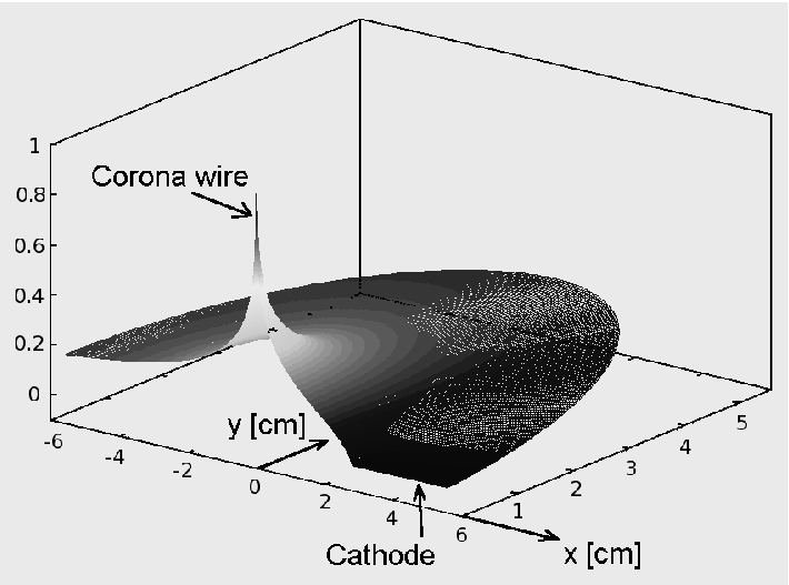
The details are worked out in the Appendix, and
Figure 4 shows the potential in a 3D plot, for
the physical values of our lifter, where is normalized to 1.
Because of the mirror symmetry around the
axis, we drew the potential only for positive .
We may derive now the electric field. For region 1 we obtain the radial field:
| (23) |
and the circular field:
| (24) |
For region 2 we obtain the radial field:
| (25) |
and the circular field:
| (26) |
It would be useful to calculate the capacitance. The charge per unit of surface on the anode is , and the charge per unit of length is given by . Clearly, the integral on zeroes the sum in eq. (23) and we are left with:
| (27) |
So the capacitance per unit of length is
| (28) |
Of course, for , from eq. (A.8) we have and we recover the known formula for the capacitance per unit of length for concentric cylinders.
We are of course interested in small , so we calculated the values of for different ratios , and fit an approximate formula for it - see Figure 5.

It comes out that for , can be expressed as
| (29) |
resulting in the following approximate formula for the capacitance per unit of length:
| (30) |
If we set the values for our lifter: and into eq. (30) we get , and multiplying by the lifter’s perimeter , the calculated capacitance comes out . To check the validity of this result we measured the capacitance of our lifter and got , which is quite close to the calculated result.
It is also useful to get a relation between the applied voltage and the field intensity on the anode. Of course, the field on the anode wire is not constant, and depends on . But for a thin anode (), the field is almost constant (see also discussion in the next section).
One may verify that for the absolute value of the sum in eq. (23) is much smaller than hence we may write the approximate expression:
| (31) |
where the second expression is a further approximation which uses eq. (29).
Again, for , , and we recover the known expression
of this relation for concentric cylinders.
In Figure 6 we show the equipotential surfaces and the field lines - those are needed in the next section.

The Warburg
[26, 27] region can
be seen also in Figure 6, and will be referred to
in the next section.
5. THE POISSONIAN PROBLEM
In this section we use the Laplacian results obtained in the previous section to solve the Poissonian problem, i.e. the state of the system when the applied voltage is bigger than the corona inception voltage.
F.W. Peek [28] made an extensive research on corona inception for different geometries like concentric cylinders, parallel wires, etc. and published the results in his book. For all the configurations involving corona around a thin wire of radius , the electric field on the surface of the wire at which corona begins (at room temperature) is given by , where with very slight variations of about for different geometries, with different asymmetries for the electric field (as found by Peek [28], page 63).
We do not have the exact value for our geometry, but as explained by Peek himself, before corona starts, the field very close to a thin wire behaves like the field on the surface (which is almost constant if the wire is thin) times the wire radius, divided by the distance from the wire. So when having the above value on the wire surface, one can easily find that at a distance of from the wire surface the field is , this way assuring a field of more than in a wide enough region around the wire to allow corona to start.
So we can safely use Peek formula:
| (32) |
as has been done a lot in the literature, for different configurations of thin wire electrode near any other electrode [11, 20, 32].
Given , we know that for our case .
Now we can find at which voltage the corona starts, i.e. the Corona Inception Voltage (CIV). The CIV is the voltage for which the Laplacian field on the surface of the corona wire equals to . For this we do not have to use Peek formula for CIV, we have the Laplacian solution for our problem. Using the approximation (31), results in or running the solution and measuring the exact relation results in , so the difference is less than . Hence we may use:
| (33) |
Because of the asymmetry around the anode, the field on the corona surface is not completely uniform, and that is the reason for the slight variations in in Peek formula for different asymmetric configurations. But fortunately, the corona wire being very thin, the field on the corona wire surface is almost uniform (up to variations of ), so we do not have to worry about it. (See also discussion before eq. (31)).
So for a voltage bigger than the CIV, the Laplacian solution is not valid anymore, and we need the solution to the Poissonian problem. This requires the simultaneous solution of eq. (3) and (2), where for we use eq. (10).
The coefficient in eq. (10) is unknown, but given the fact that the Deutsch assumption is accurate for , i.e. where the field lines are straight (see discussion in Sect. 3 and eqn. (38) and (39) in Sigmond [18]), one can iterate the coefficient in this region to get , where is the potential difference for which we solve.

The “P” prefix for Poissonian is omitted for brevity, and having a two dimensional problem represents the current per unit of perpendicular length, and represents the charge per unit of surface. The iterative calculation is done between each pair of field lines (see Figure 7) by:
| (34) |
where is at the location of , and it is known for a given , and
| (35) |
where and . Those are the numerical implementations of eq. (2) and (3). The initial condition for the iteration is Kaptzov assumption [31] (explained in the introduction), which requires:
| (36) |
After finishing the calculation between the first two field lines (i.e. in the region of very small we check the result of . Say its value is , we have to reduce by a factor of approximately 4 (approximate because the initial condition for is independent on ). This process converges very quickly (3-4 iterations), and after establishing we can process the calculations.
As explained in Sect. 3, we let drop to 0 when reaching the Warburg [26, 27] limit region (see Figure 6). Within each area element we also calculate the component of the force
| (37) |
where is the component of . The total force is eventually summed on the whole area, and knowing we sum across the line fields (in the direction), obtaining the total current .
In the final stage the force and the current are multiplied by 2 to account for the symmetric region and the values being per unit of length of the lifter, are multiplied by the perimeter . The force is normalized to show the lifted mass in grams.
The values of for which we did the calculations, have been chosen to correspond to the values on which the experiment has been done (see next section). The calculated results are presented in Table 1.
| Current [mA] | Mass that can be lifted [g] | |
|---|---|---|
| 11.12 | 0.084 | 1.54 |
| 12.9 | 0.145 | 2.65 |
| 14.08 | 0.19 | 3.55 |
| 14.4 | 0.219 | 4 |
| 15.64 | 0.27 | 4.98 |
| 16.8 | 0.34 | 6.16 |
| 18.9 | 0.46 | 8.42 |
| 20.5 | 0.586 | 10.74 |
| 21.8 | 0.678 | 12.44 |
| 22.8 | 0.76 | 13.9 |
6. THE EXPERIMENT
The diagram of the experimental setup is shown in Figure 8.

We used the lifter shown in Figure 1 for our experiments. The corona wire is a regular copper wire of radius , and the cathode is an aluminum foil of width (called and in Figure 2, respectively). The sticks that hold the device are of balsa wood, and the perimeter of the engine is . The above materials are relatively light, so that the mass of the lifter is .
For different values of resistors, the input and lifter voltages are measured and the lifting force is measured. The lifting force has been measured only for the cases for which the lifter lifted, by counter balancing it, knowing that its mass is .
The results of the measurements are shown Table 2. The current is calculated using the 2 measured voltages and the resistor.
| Lifter voltage [KV] | Source voltage [KV] | Current [mA] | Lifted mass [g] | |
| 308 | 11.12 | 25.6 | 0.047 | NA |
| 154 | 12.9 | 25.58 | 0.082 | NA |
| 110 | 14.08 | 25.51 | 0.104 | NA |
| 88 | 14.4 | 25.46 | 0.126 | NA |
| 66 | 15.64 | 25.42 | 0.148 | NA |
| 44 | 16.8 | 25.3 | 0.193 | NA |
| 22 | 18.9 | 25 | 0.277 | 7.5 |
| 10 | 20.5 | 25 | 0.450 | 10 |
| 6.8 | 21.8 | 24.92 | 0.459 | 12.2 |
| 3.3 | 22.8 | 24.8 | 0.606 | 13 |
7. COMPARISON AND APPROXIMATED FORMULAS
One may see that the calculated forces fit well to the measured forces, with an average deviation of about 6.5%. This suggests that our method gives a good estimate for the lifting force.
Let us first analyze the relation between force and current, by comparing it with a simpler case of straight, parallel and uniform field lines. If the field lines are in the direction, our coordinates (see Figure 6) correspond to respectively. For this case, applying eq. (5) and integrating over the and coordinates yields . The integral just gives the length of the field lines, let us call it , hence the force on the ionic space charge is .
Certainly, if this configuration is a parallel plates capacitor, the above force on the space charge does not produce thrust, because the wind hits one plate. But one may build a lifter with approximate straight, parallel and uniform field lines by using many thin wires on top of many flat vertical aluminum foil cathodes (see [13]). And for such a lifter describes well the thrust force.
Examining the connection between our calculated force and current in Table 1 we find that the relation between force and current is , or in terms of force instead of mass, we get . As explained above for parallel field, we would expect this relation to be proportional to , which is the distance between the electrodes in our lifter.
Hence we repeated the procedure explained in Sect. 5 for different values of , and summarized the results (which include the original value of ) in Table 3.
| Distance relative to original | Calculated | approximated by |
|---|---|---|
| 0.5 | 89.42 | 89.88 |
| 0.75 | 134.41 | 134.82 |
| 1 | 179.72 | 179.76 |
| 1.5 | 269.39 | 269.64 |
| 2 | 358.82 | 359.5 |
Obviously, one can express this relation with an excellent accuracy by:
| (38) |
Now we analyze the current-voltage relation for the calculated and measured results, which are shown in Figure 9.

Both measured and calculated results may be curve fitted with the formula
| (39) |
although the measured results look farther from their fitted curve than the calculated results (might be because of some technical problems during experiment).
The curve fitted to the calculated results used and , while this fitted to the measured results used and .
We remark that the measured results show a too high CIV and this is connected to the fact that the correspondence between measured and calculated results is poor for low currents. This might be explained by the fact that the CIV is affected by additional factors like temperature, air pressure, or partial damage to corona wire, because of repeated operation [28]. On the other hand, higher values of current and voltage are less affected by the CIV (see eq. (39)), and there we get a much better correspondence between measured and calculated current.
For a point to horizontal plane Warburg [26] found the constant to be proportional to the distance between the electrodes to the power . This power has been corrected to by Jones [38].
For concentric cylinders, Townsend [33] found the constant to be proportional to the capacitance, and the distance between electrodes at power , namely: , where is the ion mobility and is the outer cylinder radius.
We would expect our case, being two dimensional, to behave similar to Townsend’s concentric cylinders, i.e. should be some constant multiplied by . This assumption is tested with the results obtained for different values of , after curve fitting, and summarized in Table 4.
| Distance relative to original | Curve fitted | approximated by |
|---|---|---|
| 0.5 | 9.07 | 9.63 |
| 0.75 | 3.89 | 4.04 |
| 1 | 2.16 | 2.17 |
| 1.5 | 0.96 | 0.91 |
| 2 | 0.53 | 0.5 |
We see that can be expressed by the approximate formula
| (40) |
with an accuracy of about .
We may combine the eqs. (38), (39), (40), with eq. (31) and (32) to get an approximate formula for the thrust on the lifter as function of the applied voltage :
| (41) |
where all the magnitudes are in MKS units.
We remark that the mobility canceled out. This does not mean
that eq. (41) works for negative ions, because
as explained in Sect. 2, the calculations done in this paper are
valid only for positive corona.
Also we see that the force increases as the distance decreases.
CONCLUSIONS
In this paper we calculated the force on a levitation unit, built as a thin anode wire over a vertical cathode plane, as the electric force on the space charge and compared with experiment.
Our calculations were based on the Laplacian solution for this electrostatic configuration, which by itself is a new result.
With the aid of the Laplacian solution and Deutsch assumption we were able to calculate the force on the levitation unit and the current. The calculated results showed a good correspondence with the measured results.
Also, we derived for this type of lifter the relation between thrust and current in eq. (38) and the current-voltage characteristic curve in equations (39) and (40).
And finally based on the above relations, we derived an approximate formula for the force as function of the applied voltage in eq. (41).
Appendix A The calculation of the Laplacian solution
First we require condition (15):
| (A.1) |
and the above condition holds for . In this range, the functions are orthogonal, so we multiply eq. (A.1) by (for any positive integer ) and integrate on over the range . We use the following integrals:
| (A.2) |
| (A.3) |
where is the Kronecker delta. We also use:
| (A.4) |
where is a matrix defined by
| (A.5) |
The last case defined by is not likely to happen if , except for very specific values of , but we calculated this case for completeness. It is to be mentioned that for this case , for some specific and , hence is equivalent to the points or on the unity circle, so that , and this has been used in the above calculation. Also, could be written as .
After performing the above integrals, we obtain from eq. (A.1) the following result for the coefficients in eq. (20):
| (A.6) |
This result implies that are for even , and this is expected because of the mirror symmetry around the axis.
Now we require conditions (14):
| (A.7) |
The above condition is defined for . In this range, the functions are orthogonal, so we multiply eq. (A.7) by and integrate on over the range , for being any non negative integer.
First, if we do it for , the sum on the left side vanishes, and using eq. (A.2), with instead of , we obtain the following expression for :
| (A.8) |
and we could have even omitted the word “odd”, because we already know that the even coefficients from eq. (20) are .
Now we multiply eq. (A.7) by and integrate from to , for . This time vanishes, and after using , and the result (A.4) for and switched, we obtain from eq. (A.7) the following result for the coefficients in eq. (22):
| (A.9) |
We redefine now the odd indexes (like in eq. A.9) by , going from to . Hence the vector and the matrix (like in eq. A.9) are redefined to and .
We rewrite now eq. (A.6) and (A.9) in matrix form, to solve 2 matrix equations with 2 unknown vectors for the coefficients and , then find with eq. (A.8) and eventually calculate the potential and scale it by the factor .
Hence we define the diagonal matrix , by its components as , and obtain:
| (A.10) |
and we define the diagonal matrices , by , , by and , by . We also define the column vector by its components , obtaining:
| (A.11) |
We isolate from eq. (A.11):
| (A.12) |
and set it in eq. (A.10) to obtain a closed form solution for :
| (A.13) |
Clearly, for (concentric cylinders), , and are all , hence and we are left only with the trivial solution for , as expected.
References
- [1] T.T. Brown, “A method of and an apparatus or machine for producing force or motion” , British Patent 300311, (1928)
- [2] T.T. Brown, “Electrostatic motor”, US Patent 1974483, (1934)
- [3] T.T. Brown, “Electrokinetic Apparatus”, US Patent 2949550, (1960)
- [4] Website dedicated to BB effect “http://www.biefeldbrown.com/”
- [5] Jean-Louis Naudin website “http://jnaudin.free.fr/”
- [6] Tajmar M. and de Matos, C.J.,”Coupling of electromagnetism and gravitation in the weak field approximation”, Journal of Theoretics, Vol.3 (1), (Feb/March 2001).
- [7] Musha T., “Theoretical explanation of the Biefeld-Brown Effect”, Electric Space Craft Journal, Issue 31 (2000).
- [8] Website “http://montalk.net/science/84/the-biefeld-brown-effect”
- [9] T.B. Bahder, C. Fazi, “Force on an asymmetrical capacitor, Army Research Laboratory, Report No. ARL-TR-3005, (March 2003)
- [10] Tajmar M. “Biefeld-Brown Effect: Misinterpretation of Corona Wind Phenomena”, AIAA Journal, Vol.42 (2), 315-318 (2004).
- [11] L. Zhao, K. Adamiak, “EHD gas flow in electrostatic levitation unit”, Journal of Electrostatics, Vol. 64, 639-645 (July 2006)
- [12] L. Zhao, K. Adamiak, “Numerical analysis of forces in an electrostatic levitation unit”, Journal of Electrostatics, Vol. 63, 729-734 (June 2005)
- [13] Website “http://www.blazelabs.com/”
- [14] W. Deutsch, “Uber die Dichteverteilung unipolarer Ionenstrome”, Annalen der Physik, Vol. 16, 588-612 (1933)
- [15] L. E. Tsyrlin Sov. Phys.-Tech. Phys. Vol. 30 (1958)
- [16] A. Ieta, Z. Kucerovsky and W. D. Greason, “Laplacian approximation of Warburg distribution” Journal of Electrostatics, Vol. 63 (2), 143-154 (February 2005)
- [17] R.S. Sigmond, “Simple approximate treatment of unipolar space-charge-dominated coronas: the Warburg law and the saturation current”, J. Appl. Phys., Vol. 53 (2), 891-898 (1982)
- [18] R.S. Sigmond, “The unipolar corona space charge flow problem”, Journal of Electrostatics, Vol. 18, 249-272 (1986)
- [19] V. Amoruso and F. Lattarulo, “Deutsch hypothesis revisited”, Journal of Electrostatics, Vol. 63, 717-721 (2005)
- [20] J.E. Jones and M. Davies, “A critique of the Deutsch assumption”, J. Phys. D: Appl. Phys., Vol. 25 (12), 1749-1759 (1992)
- [21] A. Bouziane, K. Hidaka, J.E. Jones, A.R. Rowlands, M.C. Taplamacioglu, R.T. Waters, “Paraxial corona discharge Part 2: Simulation and analysis”, IEE Proc.-Sci. Meas. Technol., Vol. 141 (3), 205-214 (1994)
- [22] V.I. Popkov, “On the theory of unipolar DC corona”, Electrichestvo, Vol. 1, 33-48 (1949)
- [23] M.P. Sarma and W. Janischewskyj, “Analysis of corona losses on DC transmission lines. Part I unipolar lines”, IEEE Trans. Power Appar. Sysr., Vol. 88 (5), 718-731 1969
- [24] A. Bouziane, K. Hidaka, M.C. Taplamacioglu and R.T. Waters “Assessment of corona models based on the Deutsch approximation”, J. Phys. D: Appl. Phys., Vol. 27, 320-329 (1994)
- [25] J. Chen and J.H. Davidson, Plasma Chemistry and Plasma Processing, Vol. 23 (1), 83-102 (2003)
- [26] E. Warburg, “Uber die spitzenentladung”, Wied. Ann, Vol. 67 69-83 (1899).
- [27] E. Warburg, “Charakteristik des spitzenstromes”, Handbuch der Physik (Springer, Berlin), Vol. 14, 154-155 (1927).
- [28] F.W. Peek “Dielectric Phenomena in High Voltage Engineering”, McGraw-Hill (1929)
- [29] N.J. Felici, “Recent advances in the analysis of D.C. ionized electric fields”, Direct Current, Vol. 8 (10), 278-287 (1963)
- [30] M. Davies, A. Goldman, M. Goldman and J.S. Jones “Developments in the theory of corona corrosion for negative coronas in air”, Proc. XVIII Int. Conf. on Phenomena in Ionized Gases (ICPIG), (1987)
- [31] N. Kaptzov, “Elektricheskie Yavlenia v Gazakh I Vakuumme”, Ogiz, Moscow, 587-630 (1947)
- [32] J.Q. Feng, “An analysis of corona currents between two concentric cylindrical electrodes”, Journal of Electrostatics, Vol. 46, 37-48 (1998)
- [33] J. S. Townsend, Philos. Mag., Vol. 28, p83 (1914).
- [34] Y. Kondo and Y. Miyoshi, Jpn. J. Appl. Phys., Vol. 17, 643 (1978).
- [35] A. Goldman, E. O. Selim, and R. T. Waters, The 5th International Conference on Gas Discharges, lEE Conf. Publ., No. 165 pp. 88-91, (London, 1978).
- [36] E. O. Selim and R. T. Waters, Proceedings of the 3rd International Symposium on High Voltage Engineering, Paper 53.03, (Milan, 1979)
- [37] E. O. Selim and R. T. Waters, The 6th International Conference on Gas Discharges and their Applications, lEE Conf. Publ., No. 189, pp. 146-149, (London, 1980)
- [38] J. E. Jones, “A Theoretical Explanation of the Laws of Warburg and Sigmond”, Proc. Roy. Soc. London A, Vol. 453 (1960), pp. 1033-1052 (1997)