Predicting and verifying transition strengths from weakly bound molecules
Abstract
We investigated transition strengths from ultracold weakly bound 41K87Rb molecules produced via the photoassociation of laser-cooled atoms. An accurate potential energy curve of the excited state was constructed by carrying out direct potential fit analysis of rotational spectra obtained via depletion spectroscopy. Vibrational energies and rotational constants extracted from the depletion spectra of 41–50 levels were combined with the results of the previous spectroscopic study, and they were used for modifying an ab initio potential. An accuracy of 0.14% in vibrational level spacing and 0.3% in rotational constants was sufficient to predict the large observed variation in transition strengths among the vibrational levels. Our results show that transition strengths from weakly bound molecules are a good measure of the accuracy of an excited state potential.
pacs
34.20.-b,33.15.Bh,37.10.Mn,82.80.MsI Introduction
Ultracold molecular gas is a prominent candidate for realizing novel distinctive applications in physics and chemistry, including precision measurements, quantum computation, ultracold chemistry, and novel quantum phases [1, 2]. Thus far the production of ultracold molecules in the vibrational ground state has been dependent on the optical transfer of weakly bound molecules formed via either photoassociation [3] or magnetoassociation [4]. Among the previously proposed methods [5, 6, 7, 8, 9, 10], stimulated Raman adiabatic passage (STIRAP) [11, 12, 13] of weakly bound molecules is the most efficient method for preparing a molecular sample in a single quantum state.

In the STIRAP transfer, an excited state is used as an intermediate state. It is important to select an excited state having large transition strengths from both weakly bound and deeply bound levels. In general, the strengths of molecular transitions from low vibrational levels are readily predicted on the basis of the Franck-Condon factors (FCFs) calculated from a potential energy curve or molecular constants [14]. The small number of nodes in the radial wavefunction for a low vibrational level indicates a low sensitivity to deviations in the radial direction, thereby enabling us to explain the intensity distribution over vibrational levels from molecular constants. However, it is difficult to predict transition strengths from weakly bound molecular levels because weakly bound levels have a large number of nodes in their wavefunctions; hence, the FCFs are quite sensitive to the wavefunctions of excited states. In this letter, we show that transition strengths from weakly bound levels can be predicted on the basis of an accurate potential energy curve of the excited state, constructed via direct potential fit (DPF) analysis [15] of both vibrational energies and rotational constants.
We focused on the state of KRb in the range 11400–11800 cm-1 with respect to the ground atomic threshold, which was proposed as a potential candidate for the STIRAP transfer of weakly bound molecules to the rovibrational ground state [16]. An RKR potential curve of the state was reported from the potential minimum up to 10400 cm-1 [17, *amiot2000corrigendum]. An ionization spectrum for 39K87Rb obtained by using a pulse laser and a depletion spectrum near 11700 cm-1 is provided in Ref. 16. Recently, we have realized the STIRAP transfer of weakly bound molecules (, of ) to the rovibrational ground state (, of ), mediated by the level of the state [19]. Before conducting this experiment, we carried out depletion spectroscopy in the range 11400–11800 cm-1, which revealed 10 vibrational levels. We found that the width of the observed spectra was highly dependent on the vibrational levels of the state. By introducing an analytical representation for power broadening, we extracted the transition strengths for each vibrational level. The other electronic states that correlate with the state via spin-orbit interaction were far away; hence we assumed that most of the perturbations from these electronic states were negligible. Thus, we could analyze the experimentally obtained spectra on the basis of a single potential curve. In addition to the previous spectroscopic work near the bottom of the potential [17, *amiot2000corrigendum], vibrational energies and rotational constants extracted from the spectra were used to construct an accurate potential via DPF analysis. Using the modified potential, it was possible to explain the variation in transition strengths among the vibrational levels of the state in terms of the FCFs.
II Depletion spectroscopy
Previously, our experimental setup for the spectroscopy of ultracold 41K87Rb molecules was described in detail [20]. We provide a brief summary herein. We started with a dual-species magneto-optical trap (MOT) of 41K atoms and 87Rb atoms. A compressed MOT (C-MOT) procedure was applied for 40 ms to compress and cool the 41K and 87Rb atoms. The typical densities and temperatures of 41K and 87Rb at the end of C-MOT were cm-3 and 400 K and cm-3 and 100 K for 87Rb, respectively. A photoassociation (PA) laser (wavenumber, 12570.13 cm-1; intensity, Wcm-2) was applied for 10 ms at the end of the C-MOT process. The produced molecules were detected using micro-channel plates (MCP) after they were ionized via resonance enhanced multi-photon ionization (REMPI) using a pulsed dye laser (wavenumber, 16543 cm-1; intensity, 3 W cm-2).
Depletion spectra were obtained by monitoring ion counts in the level of , while a CW Ti:Sapphire laser (Sirah Matisse TX; intensity, 50 Wcm-2; beam waist, 350 m) was continuously applied and scanned. In the present study, we analyzed spectra for the , level, whose binding energy with respect to the atomic threshold =1+=1 was measured as cm-1. The frequency of the Ti:Sapphire laser was monitored using a Fabry-Perot cavity which was locked to 87Rb D2 line. The cavity transmission signal was used to calibrate the variation in the scanning speed and to measure the relative frequency of the laser with respect to the cavity transmission peak with a precision of 3 MHz. The absolute frequency was measured using a commercial wavemeter (Wavelength WS-7; accuracy, 60 MHz). The accuracy of measurements for rotational constants was limited by the spectral width, which was of the order of 100 MHz, whereas that for vibrational energies was limited by both the spectral width and the wavemeter.

Fig. 2 shows a depletion spectrum for the level of the state, which was used as an intermediate state for the STIRAP transfer from the , level of to the , level [19]. We can extract transition strengths as well as rotational constants for both ground and excited states from the spectra. In the appendix, we show that an approximate representation of the full-width-half-maximum (FWHM) of a depletion spectrum is given by
| (1) |
where is the Rabi frequency; , the natural width of the excited state; and , the duration of spectroscopy. Roughly speaking, the width increases not only with the light intensity but also with the duration of spectroscopy. In our case, the duration was estimated as a few milliseconds on the basis of the temperature of the molecules and beam diameter of the depletion laser. The natural width of the state was not precisely known, but it was obtained as 2 kHz from an ab initio calculation [21]. In the following discussion, we derive the Rabi frequency from the observed spectrum by assuming as 2 ms, as 2 kHz, and as 60.
III Analysis

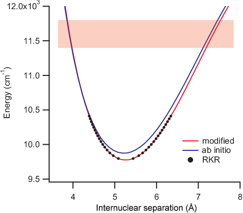
Although the ab initio potential [22] enabled us to identify the symmetry of the observed spectra without any ambiguity, it gave rotational constants that exceeded the experimental ones by approximately 1% (Fig. 3). There were two reasons for this deviation. First, the potential minimum exceeded the minimum of the RKR curve by 97 cm-1. Second, the outer turning point was at the shorter internuclear separation than the RKR potential. We found that the variation in the observed transition strengths could not be understood with the ab initio potential. The observations could not be attributed to the small change in the vibrational quantum number, which corresponded to the energy difference in the minimum of the RKR and the ab initio potentials. These facts indicate that the ab initio potential is inaccurate. In order to obtain an accurate potential, we carried out DPF analysis, whereby a potential is iteratively modified until its eigenvalues coincide with those determined from the experimental spectra [15]. With the aid of the phiFIT program code [23], we first constructed an analytical Extended Morse Oscillator (EMO) potential of the state on the basis of (1) the RKR curve, (2) a few points from the inner curve of the ab initio potential, and (3) a few points around 12500 cm-1 from the outer curve of the ab initio potential. The potential curve of the ground state was also required for the calculations. We used an EMO potential fitted to an accurate, experimentally determined potential [24]. Then, the analytical potential of the state was modified to reproduce our data by using the DPotFit program code [25]. A good convergence was achieved when we modified the potential significantly by manually moving the points from the ab initio potential. This procedure was repeated until the eigenvalues of the potential were within 0.05 cm-1 of the observed levels, i.e., only 0.14% of the vibrational level spacing. The remaining deviations were presumably due to the incomplete analytical function used to represent the potential. Table 1 lists the final potential parameters. These parameters are used to represent the potential energy curve in the following form:
| (2) |
| Parameter | Value | Parameter | Value |
|---|---|---|---|
| 9777.6963 | -0.804673587 | ||
| 3246.0363 | 3.00474008 | ||
| 5.25904119 | 11.3877324 | ||
| 0.449794066 | -2.140717462 | ||
| 0.200265883 | -39.73110586 | ||
| 0.406840126 | -17.01400311 | ||
| 0.207884795 | 50.93279647 | ||
| -0.476349301 | 44.83137419 |
| E (cm-1) | B (cm-1) | |||||
|---|---|---|---|---|---|---|
| Obs. | ab initio - Obs. | Mod. - Obs.() | Obs. | ab initio - Obs.() | Mod. - Obs. () | |
| 41 | 11428.965 | -1.5 | 2.5 | 2.067 | 1.9 | -7.0 |
| 42 | 11466.644 | -1.6 | 29.9 | 2.056 | 2.3 | -1.7 |
| 43 | 11504.193 | -1.8 | 42.6 | 2.05 | 2.4 | -1.5 |
| 44 | 11541.484 | -1.9 | 164.2 | 1.99 | 7.8 | 52.6 |
| 45 | 11578.919 | -2.2 | -11.4 | 2.038 | 2.4 | -1.5 |
| 46 | 11616.036 | -2.4 | -28.0 | 2.037 | 1.8 | -6.8 |
| 47 | 11652.982 | -2.6 | -37.3 | 2.027 | 2.2 | -3.2 |
| 48 | 11689.751 | -2.7 | -37.5 | 2.017 | 2.5 | 0.3 |
| 49 | 11726.308 | -2.7 | 1.2 | 2.008 | 2.9 | 2.5 |
| 50 | 11762.685 | -2.7 | 43.0 | 2.005 | 2.5 | -1.4 |
Fig. 4 shows the RKR potential, ab initio potential and modified potential. At the new potential, rotational constants were reproduced within 0.3% of the observed values (Table 1). We excluded the level from the analysis because the characteristics of this level are anomalous; a much larger transition strength, a much smaller rotational constant, and a much larger deviation in a vibrational energy were observed at this level. These features indicate that this level was coupled to the state which was observed at 1 cm-1 above the level.

The most important implication of this analysis is that the variation in the transition strengths with respect to the vibrational levels of the excited state can be accurately explained on the basis of the new potential. Fig. 5 shows a plot of the Rabi frequencies derived from the observed spectra against those calculated from the corrected potential. For comparison, the same plots based on the ab initio potential are also shown. The calculated values are calibrated on the basis of our recent measurement of the transition dipole moment between , and , , , determined via dark resonance spectroscopy of the rovibrational ground-state molecules. Weakly bound molecules have more than 90 nodes in their wavefunction; hence, the FCFs are highly dependent on the wavefunction of the excited state. In other words, the FCFs can serve as a sensitive measure of the accuracy of wavefunctions. Our results show that accuracies of 0.14% in vibrational level spacings and 0.3% in rotational constants are sufficient to predict the FCFs from weakly bound levels; these values are justified by considering the typical size of nodes in the radial wavefunction. On one hand, the weakly bound level in the ground state has an outer turning point of 10 Åand an inner turning point of 2 Åin the internuclear distance. Within these two points, there are 91 nodes; hence each node has a typical size of 0.1 Å. Therefore, the required accuracy for representing the wavefunction is 10-2 Å. On the other hand, in the present analysis, an accuracy of 0.3% in rotational constants or 0.15% in internuclear distance is obtained for the state because the relation between the rotational constant and the internuclear distance is given by . Assuming the typical size of molecules in the 41–50 levels of as 6 Å, we can derive the accuracy of the modified potential in the radial direction as 10-2 Å; this value is in good agreement with the required accuracy for representing the weakly bound level.
Now that we obtained an accurate potential curve as well as the absolute values of the transition dipole moment of the , level with the and levels of , we can predict the transition dipole moment for each transition. Fig. 6 shows our prediction for the transition dipole moments of the state with the least bound state and for those with the lowest rovibrational level . The level used in Ref. 19 has favorable wavefunction overlaps with both the weakly bound and the lowest rovibrational levels; however other levels such as and can potentially serve as an intermediate state for the STIRAP transfer of weakly bound molecules to the rovibrational ground state. The potential presented herein can enable an accurate prediction for other isotopic combinations of KRb. Further, the present method for achieving an accurate potential and verifying its accuracy can be extended to other molecular states that exhibit significant spin-orbit mixing by evaluating eigenvalues via coupled channel calculations including spin-orbit interaction.

IV Conclusion
The state of KRb was investigated via the depletion spectroscopy of ultracold molecules formed by the photoassociation of laser-cooled 41K and 87Rb atoms. The spin-orbit mixing of other electronic states with the state was negligible; hence, we could assume this state as a single potential. The simplicity of the state enabled us to modify the potential to reproduce our observations as well as to assign the spectra. We observed 10 vibrational levels in the range 11400–11800 cm-1 with respect to the ground atomic threshold. We developed a theoretical model that related the spectral width with the Rabi frequency, which was used to compare the transition strengths for each vibrational level. Rotational constants extracted from the observed spectra showed a 1% deviation from those calculated using an ab initio potential. By carrying out DPF analysis, we constructed an accurate potential that reproduced energy levels with an accuracy of 0.14% in vibrational level spacing and 0.3% in rotational constants. The variation in transition strengths among vibrational levels could be understood in terms of FCFs calculated with the modified potential. Our results indicate that the transition strengths from weakly bound levels serve as a sensitive measure of wavefunctions, which can be used to test the accuracy of the potential curve. In general, the proposed procedure can be adopted for constructing an accurate potential and verifying its accuracy on the basis of rotational spectra for weakly bound molecules.
*
Appendix A Analytical expression for the line shape of a depletion spectrum

We consider a general situation, as shown in Fig. 7, and we assume that radiative transitions occur much faster than the time variation of the population in each molecular level because of the photoassociative creation of molecules. We first consider the evolution of the population in the ground and excited states of a single molecule. The optical Bloch equation for this system can be written as
| (3) |
where , , and and denote an excited state and a weakly bound level, respectively. and denote the detuning frequency and the Rabi frequency, respectively. The decay rates from the excited state to the initial weakly bound level and to other levels are given by and , respectively. The photoassociation rate is denoted by . The width is much larger than the Rabi frequency in the experiment; hence, we can assume that the time evolution of and is much slower than that of . Thus, we can set and obtain the following expression for :
| (4) |
Substituting Eq.(4) in Eqs.(3), we obtain alternative equations for and as
Here, we assume that the time taken by the mean value of the population ratio to attain a constant value after is greater than the typical time for radiative transitions. By using the relation , Eqs.() give following equations:
Substituting the first equation in the second equation, we obtain a time-independent equation for :
| (7) |
This equation is readily solved, and it gives the following expression for .
| (8) |
This expression is used in the following discussion. Next, we derive rate equations for the population in the ground and excited molecular levels for the number of molecules:
| (9) |
where and denote the number of molecules in the ground and excited states, respectively, and is the total number of molecules. In these rate equations, a typical timescale is of the order of 1 ms, and it is governed by . This is much longer than the typical timescale for radiative transitions in most cases (1 s). The time evolution of is given by
| (10) |
Thus, the solution for is given by
| (11) | |||||
This expression gives the line shape of a depletion spectrum for a duration . Assuming , Eq.(11) gives
| (12) |
on resonance ( and ), whereas at an infinite detuning ( and ) is given as
| (13) |
at an infinite detuning is much larger than on resonance. Thus, the width of the spectrum is determined by finding such that it satisfies
| (14) |
Substituting Eq.(11) in Eq.(14) and rewriting the equation with a new variable , we obtain the following equation:
| (15) |
A rigorous solution of this equation is given by
| (16) |
where W is the Lambert W function. Thus, the parameter in Eqs.(8) is given by
| (17) |
Assuming , we obtain the following expression for FWHM:
| (18) |
When decays from the excited state to the initial state are negligible , we obtain a simple relation (1). It is difficult to evaluate the numerical factor precisely; therefore, the width of a depletion spectrum cannot serve as an accurate measure of the transition strength. However, the expression (1) enables us to systematically compare transition strengths for different vibrational levels.
Acknowledgements.
We thank P. Naidon and T. Kishimoto for insightful discussions, and K. Oasa, Y. Tanooka, and K. Mori for their assistance with the experiment. K. A. and D. A. acknowledge the support of the Japan Society for the Promotion of Science.References
- [1] R. V. Krems, W. C. Stwalley, and B. Friedrich, Cold molecules: theory, experiment, applications (CRC, Boca Raton, 2009).
- [2] L. D. Carr, D. DeMille, R. V. Krems, and J. Ye, New J. Phys. 11, 055049 (2009).
- [3] K. M. Jones, E. Tiesinga, P. D. Lett, and P. S. Julienne, Rev. Mod. Phys. 78, 483 (2006).
- [4] T. Kohler, K. Goral, and P. S. Julienne, Rev. Mod. Phys. 78, 1311 (2006).
- [5] J. M. Sage, S. Sainis, T. Bergeman, and D. DeMille, Phys. Rev. Lett. 94, 203001 (2005).
- [6] M. Viteau et al., Science 321, 232 (2008).
- [7] J. Deiglmayr et al., Phys. Rev. Lett. 101, 133004 (2008).
- [8] K.-K. Ni et al., Science 322, 231 (2008).
- [9] F. Lang et al., Phys. Rev. Lett. 101, 133005 (2008).
- [10] J. G. Danzl et al., Nat. Phys. 6, 265 (2010).
- [11] K. Bergmann, H. Theuer, and B. W. Shore, Rev. Mod. Phys. 70, 1003 (1998).
- [12] N. V. Vitanov, M. Fleischhauer, B. W. Shore, and K. Bergmann, Adv. At. Mol. Opt. Phys. 46, 55 (2001).
- [13] P. Kral, I. Thanopulos, and M. Shapiro, Rev. Mod. Phys. 79, 53 (2007).
- [14] G. Herzberg, Molecular spectra and molecular structure. 1. Spectra of diatomic molecules (Van Nostrand, New York, 1950).
- [15] J. Seto, R. Le Roy, J. Vergès, and C. Amiot, J. Chem. Phys. 113, 3067 (2000).
- [16] D. Wang et al., Phys. Rev. A 75, 032511 (2007).
- [17] C. Amiot, J. Vergès, J. d’Incan, and C. Effantin, Chem. Phys. Lett. 315, 55 (1999).
- [18] C. Amiot, Chem. Phys. Lett. 318, 289 (2000).
- [19] K. Aikawa et al., Phys. Rev. Lett.(in press) (2010).
- [20] K. Aikawa et al., New J. Phys. 11, 055035 (2009).
- [21] R. Beuc et al., J. Phys. B 39, S1191 (2006).
- [22] S. Rousseau, A. R. Allouche, and M. Aubert-Frecon, J. Mol. Spectrosc. 203, 235 (2000).
- [23] R. J. Le Roy, “A Computer Program to Fit Pointwise Potentials to Selected Analytic Functions,” (2007), current version is betaFIT 2.0, available at http://leroy.uwaterloo.ca/programs.html.
- [24] A. Pashov, O. Docenko, M. Tamanis, R. Ferber, H. Knockel, and E. Tiemann, Phys. Rev. A 76, 22511 (2007).
- [25] R. J. Le Roy, J. Y. Seto, and Y. Huang, “A Computer Program for Fitting Diatomic Molecule Spectral Data to Potential Energy Functions,” (2006), available at http://leroy.uwaterloo.ca/programs.html.