Fairness in overloaded parallel queues
Abstract
Maximizing throughput for heterogeneous parallel server queues has received quite a bit of attention from the research community and the stability region for such systems is well understood. However, many real-world systems have periods where they are temporarily overloaded. Under such scenarios, the unstable queues often starve limited resources. This work examines what happens during periods of temporary overload. Specifically, we look at how to fairly distribute stress. We explore the dynamics of the queue workloads under the MaxWeight scheduling policy during long periods of stress and discuss how to tune this policy in order to achieve a target fairness ratio across these workloads.
1 Introduction
Queueing systems are generally designed with sufficient allocation of resources to ensure that the system is stable. Subsequently, a large body of research in queueing has focused on characterizing the stability region and on evaluating and optimizing performance when the queues are operated within this region. However, in reality, it is inevitable that a system will repeatedly enter long periods of overload, either due to an unpredictable increase in load or because some service resources may become unavailable/breakdown. In such periods, which may last for a fairly long duration of time, the system may have more load than it can handle. Hence, it is natural to want to understand what happens during these periods of temporary instability.
Some examples of real systems which experience periods of instability can be found in internet communication networks, hospitals, and call centers. Consider systems where traffic is bursty. For instance, in communications networks, with the release of a new online game, the system may be over-stressed as many people attempt to simultaneously enter the virtual world. At a hospital, there may be a surge in demand for the limited hospital resources during a catastrophic event or viral outbreak. In these cases, the system load may increase to potentially unstable levels. A separate scenario of temporary overload may occur when resources are lost. In call centers, a power outage may effectively remove a pool of servers. Consequently, while the system load may remain constant, the available service resources have been reduced, stressing the system.
In long periods of overload, it is inevitable that the system backlog will grow significantly, so the question of performance optimization becomes moot. However, it is desirable to share the stressed resources in a fair manner among the different customers. In this paper, we study fair resource allocation in multiclass parallel server queues during long periods of overload or temporary instability.
How does one define fairness in an overloaded system? Consider a system which is overloaded for a very long time window. During this time window, the system is essentially unstable, so that the total backlog grows without bound. However, it is plausible that some customer classes will enjoy a greater allocation of the stressed resources, enough such that the system will appear stable to these classes. This is unfair. Our novel notion of fairness requires that the backlog of the different customer classes will grow large according to a predetermined proportion, thereby proportionately distributing stress across customer classes. This is the same as requiring that the backlog vector will grow along a prespecified direction.
Working with this notion of fairness, our ultimate goal is to determine how to operate the overloaded system such that the total backlog is minimized subject to a fairness constraint. Our main result is that the MaxWeight scheduling algorithm, with carefully selected weight parameters, will achieve this goal asymptotically, as the duration of the overloaded period grows large. The MaxWeight policy selects, at each time point, a service configuration which maximizes the aggregate service rate weighted by the queue backlogs and a controllable weight vector (Tassiulas and Ephremides 1992, Mandelbaum and Stolyar 2004). MaxWeight has been shown to be throughput maximizing (see for example Tassiulas (1995), Tassiulas and Bhattacharya (2000), McKeown et al. (1999), Armony and Bambos (2003)). That is, as long as the system is stabilizable, it will be stable under MaxWeight.
Our analysis first shows that, under MaxWeight with arbitrary fixed weights, the backlog in an overloaded system will grow to infinity according to a well defined direction. We then proceed to show that this direction can be turned to any feasible fairness proportion by carefully selecting the weight parameters of MaxWeight. Finally, we establish that, in the limit, MaxWeight will minimize the total backlog among all algorithms that obtain this fairness direction.
The approach we take in our analysis is a trace-based approach (Loynes 1963, Armony and Bambos 2003, Ross and Bambos 2009) which analyzes individual traces of customers’ arrival times and workload requests. To show that the backlog grows along a specific direction, we use direct geometric arguments that examine the dynamics of an actual trajectory of the backlogs and how it evolves over time. In particular, our statistical assumptions are extremely mild, and only require that the workload entering the system has a well defined long time average.
The rest of the paper is organized as follows: We conclude this introduction by surveying some closely related literature. In Section 2 we formally introduce our queueing model and the notion of fairness which we study. In Section 3 we show the existence of a unique limit for the queue backlogs when the system is unstable. In Section 4 we discuss how to control the backlog to achieve our desired fairness criterion. In Section 5 we show some numerical results to demonstrate the performance of our proposed algorithm in practice. Finally, we conclude in Section 6.
Related Literature
Stolyar (2004) analyzes the same type of parallel server queueing systems, under the assumption that the system is in heavy-traffic. That is, the system is stable but operates close to the boundary of the stability region. For such systems, the author shows that under MaxWeight and a complete resource pooling condition, the backlog vector will experience a state-space collapse, which implies that it will asymptotically follow a well defined direction. The author also shows that MaxWeight minimizes the workload, where the latter is defined as the total backlog weighted by the above direction. These results are similar to our convergence and backlog minimization results, but since the system considered in Stolyar (2004) is not overloaded, much stronger assumptions are required there–such as the Markov property and the complete resource pooling condition. Mandelbaum and Stolyar (2004) generalizes these results for convex holding cost functions and a corresponding generalized rule.
More recently, Shah and Wischik in (Shah and Wischik 2011) study the asymptotic behavior of fluid models in overload under MaxWeight and other policies. Analogously to our result, they show that as time grows large, the fluid vector will approach a well defined direction. While the network structure and the set of policies that Shah and Wischik (2011) studies are more general than our setting, that paper focuses on characterizing the asymptotic direction of the backlog of the overloaded system. Our paper, on the other hand, focuses on controlling this direction to satisfy a fairness constraint and on minimizing the backlog subject to this constraint. Methodologically the two papers are also different; Shah and Wischik (2011) uses Lyapunov functions to prove convergence of the continuous fluid trajectory, while our analysis directly examines the dynamics of the queueing trajectory.
Also in the networked setting, Georgiadis and Tassiulas (2006) consider overloaded sensor networks where transmissions are scheduled in a distributed manner. Specifically, Georgiadis and Tassiulas (2006) show that a policy analogous to the Adaptive Back Pressure policy of Tassiulas (1995) (reference [20] in Tassiulas’ paper) obtains, in the limit, a backlog vector which is the so-called ”most balanced” among all feasible limits, in overload. Similar to Shah and Wischik (2011), the authors consider a fluid model rather than the direct queueing trajectory dynamics considered in this work.
Our concept of fairness in this paper is also somewhat unusual. Two commonly used fairness criteria are Max-Min and Proportional Fairness. A system is considered Max-Min fair if the utility of the user with the minimum utility is maximized. On the other hand, a system is considered to be proportionally fair if the amount of service resources a user is allocated corresponds to the proportion of anticipated resource consumption required by the user. These two notions of fairness can be tied together under the description of -fairness with different values of (Mo and Walrand 2000). There has been a substantial amount of work in the development of scheduling policies which ensure some fairness criteria (see Mo and Walrand (2000), Kelly and Williams (2004), Eryilmaz and Srikant (2005), Neely et al. (2005), Eryilmaz and Srikant (2006), Neely (2006), Bonald et al. (2006), Massoulie (2007) and related works). A common thread in those papers is an assumption of stability, whereas we consider fairness during periods of temporary instability. We define fairness by a set of ratios which specifies the desired proportion of the aggregate backlog each queue contributes. In Section 4.4 we elaborate more on the connection between the traditional notions of fairness and the one used here.
Perry and Whitt (2009), Perry and Whitt (2011) consider how to deal with unexpected overload. They consider overload in the setting of two initially separated service systems which share resources when one becomes overloaded. Using a fluid model, they consider how to share resources across the two systems in order to maintain a constant ratio between the two queues. Our setting is quite different as there is a single system with multiple parallel queues. However, we share a similar control goal of maintaining a constant ratio between queues, of which we may have more than two.
2 The Queueing Model
We consider a queueing system with queues and service vectors. New jobs arrive to the system and are queued up to be served. The system administrator dynamically selects which service configuration to implement for service of available jobs in the queue. We consider how to make this selection in a ‘fair’ manner, where we will be more precise as to what we mean by fair in the coming discussion.
More formally, we consider a queueing system with parallel queues, indexed by . Time is discrete and indexed by . Let be the number of jobs arriving to queue in time slot . We assume that for some arbitrarily large . For each , we assume that
| (2.1) |
is well-defined, positive, and finite. The arrival vector in time slot is thus
| (2.2) |
with corresponding long-term traffic load vector:
| (2.3) |
Arriving jobs are buffered in their respective queues and are served in a first-come-first-served (FCFS) manner within each queue.
In each time slot, a service vector is selected to be used. Each service vector is a -dimensional vector:
| (2.4) |
where is the number of jobs removed from queue in a single time slot when service configuration is used.
The workload in queue at time is denoted by with corresponding workload vector:
| (2.5) |
This corresponds to the number of jobs in each queue in time-slot .
Given workload vector and service configuration , the number of jobs that are served and depart from queue is:
| (2.6) |
where the minimum accounts for the fact that jobs can only be serviced if they are already waiting in the queue. Hence, if , there is some idle service provided by service vector due to the lack of available jobs to be processed. The workload vector evolves as:
| (2.7) |
Assuming the queue begins empty at time , then the workload vector is given by:
| (2.8) |
Applications
We note that many applications of interest can be modeled in this way. For example, in communication networks, the backlogs correspond to packets waiting to be transmitted on various wired or wireless links while the service vectors correspond to various packet switch configurations. In call centers, the backlogs correspond to the number of customers of various classes waiting to be served while the service vectors correspond to specific allocations of staff with differing skills to each customer class.
2.1 (In)Stability Region
Loosely speaking, we consider a system to be rate stable if the average job departure rate is equal to the average arrival rate. We define the stability region of a system, , such that if , then there exists some policy which guarantees for each queue, , that:
| (2.9) |
The stability region can be characterized as:
| (2.10) | |||||
as defined in Ross and Bambos (2009). Hence, any system load which is dominated by a convex combination of service vectors is stablizable. Furthermore, stability is ensured by using this convex combination.
When the system load is outside of the stability region, then the system is unstable. Hence, if , then there does not exist any policy which guarantees that:
| (2.11) |
and with probability ,
| (2.12) |
for some (see Armony and Bambos (2003)). We refer to this as the instability region. Consider the following simple example of the stability and instability regions.
Example 1
Consider an example with two queues () and three () service vectors:
| (2.13) |
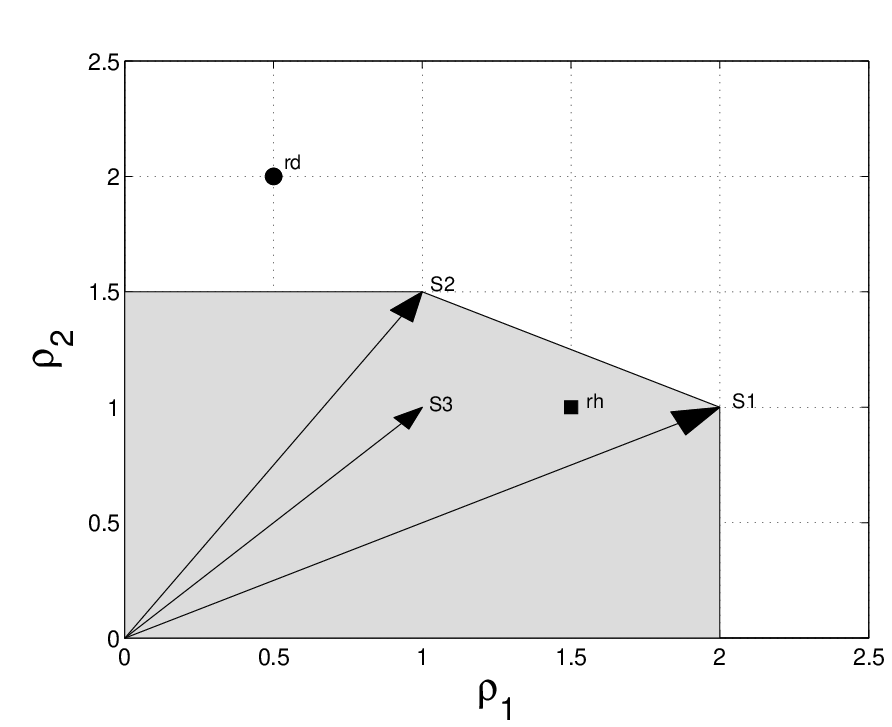
The stability region, , is given by the convex hull of (and their projections onto the axes). Note that is a non-essential service vector, since it is dominated by a convex combination of and and its removal would not change . Any load vector within the shaded region in Figure 1 is stabilizable; outside the region, is not. Hence, is stabilizable while is not.
The focus of this work is the understand and control the dynamics of systems which are temporarily overloaded over a long time horizon. To do this, we approximate the dynamics of a temporarily unstable system with a system which is permanently unstable (). When the period of overload is long enough, the dynamics of the two systems will be similar. Hence, our analysis focuses on the dynamics of unstable systems.
2.2 Fairness
The goal of this work is to determine a service discipline which allows us to fairly serve queues when the system is temporarily overloaded (). There are many different definitions of fairness (see for instance Mazumdar et al. (1991), Kelly et al. (1998), Mo and Walrand (2000)). In this paper, we focus on a notion of fairness where the workloads grow according to a fixed proportion. More formally, we assume we are given a set of ratios . These ratios specify the proportion of the aggregate workload which each queue contributes. Whenever , the goal is to control the workload such that for large :
| (2.14) |
More precisely, we want to control such that:
| (2.15) |
where satisfies our fairness criterion:
| (2.16) |
defines a direction which we want the backlogs to grow; includes the scale factor to specify how quickly they grow.
There may be many policies which achieve this fairness criterion and our goal is to find the policy which achieves it with the minimal workload. Let correspond to the workload at time given service vector is used in time slot . Our goal is to find such that for large :
| (2.17) |
Furthermore, if there exists which uses in time slot and , then
| (2.18) |
We will go into more detail about this fairness criterion in Section 4. Further, we will show that this definition can be generalized to other fairness definitions. Our proposal is to use MaxWeight scheduling policies to achieve our fairness criterion Armony and Bambos (2003), Ross and Bambos (2009).
2.3 The MaxWeight Scheduling Policy
The stability region guarantees the existence of a stabilizing policy. We now briefly review a family of stabilizing policies, which we refer to as MaxWeight Scheduling. This is the special case of Projective Cone Scheduling (PCS) when projection matrices are diagonal. This family of policies is characterized by service cones wherein the set of workloads under which service vector is used forms a cone in the workload-space. We focus on this family of policies because they work ‘well’, i.e. are stabilizing when possible, they are simple to implement, and as we will see later, they are optimal in the sense that they obtain the minimum backlog (2.18) subject to the fairness criterion (2.17).
Let be a symmetric, positive definite matrix with non-positive off-diagonal elements. Let be the workload at time . Then, the PCS algorithm selects service vector :
| (2.19) |
It is shown in Ross and Bambos (2009) that the PCS policy is rate stable for any . This policy is also desirable from an implementation standpoint as it only requires current information (workload state) and does not require knowledge of the system load .
We define the service cone as the set of workload vectors, , such that service vector is used under the algorithm defined by positive definite matrix ; i.e.:
| (2.20) |
For the rest of the discussion, we will suppress the dependence of the service cones on the matrix .
Throughout this work, we will focus on the case where the matrix is a diagonal matrix, (and positive-definite, hence, all its diagonal elements are positive). This specifies the set of algorithms to MaxWeight scheduling algorithms, which have been studied extensively in the past.
Assumption 2.1
is a diagonal, positive definite matrix, i.e. and ,
While we are ultimately interested in the behavior of this queueing system when it is temporarily overloaded, our focus on MaxWeight scheduling policies ensures that the system is stabilized when possible. We will examine the asymptotic behavior of this class of policies and its implications in term of our fairness criterion. We will see that this family of algorithms allows us to satisfy certain fairness criterion by manipulating the matrix. Furthermore, we will see in Section 4.2 that the MaxWeight scheduling policies achieves the lowest workload which satisfies our fairness criterion. In order to see this, we must first understand how the matrix affects the asymptotic behavior of our queueing system.
3 Asymptotic Dynamics in Overload
Before we consider how to control the workload vector, , we first begin by building an understanding of its asymptotic dynamics given diagonal MaxWeight matrix . We already know that if , then the MaxWeight scheduling policy stabilizes the system and the workload is always finite. On the other hand, many real systems enter periods of instability where the system load is temporarily outside of the stability region. From Armony and Bambos (2003), when the workload explodes: . However, we are interested in finding out how exactly this happens. Is there a finite limit for ? If so, what is it and what does it depend on? This section is devoted to answering these questions.
Suppose that the system operates in overload, in the sense that , where
| (3.1) |
as defined in Ross and Bambos (2009). We consider the limit defined below:
| (3.2) |
and select a convergent increasing unbounded subsequence on which the ‘’ is attained11 1 See footnote 12 of Ross and Bambos (2009) concerning why such a subsequence exists – hence,
| (3.3) |
and
| (3.4) |
Lemma 3.1
We have
| (3.5) |
Proof: See the proof of Proposition 2.1 in Armony and Bambos (2003). In short, we have that
| (3.6) |
This in turn implies that:
| (3.7) |
This result follows directly from the stability results of Armony and Bambos (2003), Ross and Bambos (2009) which say that when the time-scaled backlog goes to 0 as . When the system is not stable, the opposite occurs and there exists a non-zero sub-limit. Our key result in this section is that is the unique limit of over all possible arrival traces.
Theorem 3.1
When , we have
| (3.8) |
That is, the workload explodes on the same non-zero ray on any arrival trace. Furthermore, is defined as the unique solution to the following convex program:
| (3.9) |
where
| (3.10) |
and is the stability region given by . Therefore, with and for each , where is the set of service vectors. Equivalently, is the unique fixed point which satisfies with and
| (3.11) |
Proof: The proof will conclude at the end of Section 3. We will first show that the limit is unique for each individual arrival trace. We then extend our analysis to show the limit is the same for all arrival traces with identical time-average traffic load, , which in turn, implies uniqueness over all arrival traces. We begin with a number of definitions and structural properties of the defined elements.
From Section V of Ross and Bambos (2009) on MaxWeight Scheduling cone geometry, recall that is a cone, and when (the interior of ) the MaxWeight scheduling policy will choose . Moreover, the surrounding cone of any non-zero vector is the cone
| (3.12) |
where is the set of service vectors of that MaxWeight Scheduling would select for backlog and is the set of non-essential ones (see Ross and Bambos (2009), end of Section IV). Loosely speaking, the non-essential service vectors are the one whose removal will not change the stability region. Hence, is the union of all cones corresponding to the set of service vectors which can be used if . We have
| (3.13) |
where is the interior of . Define now
| (3.14) |
which is the set of backlogs such that no queue with can be emptied in a single time slot. Note that is upward-scalable; indeed, implies for any scalar . Note that when we have for all with , so . Therefore,
| (3.15) |
That is, all service capacity allocated at slot to queue with is used; there is no idling in that time slot; and the departures from all queues with is exactly equal to the total service provided to that queue. Consider now the set
| (3.16) |
and note that it is upward-scalable, that is, implies for any scalar . Thus, the set is ‘cone-like’.
The main idea for the proof for the existence of our limit is that excursions away from take a very long time–so long that the time-average properties we have for arrivals will become active. In particular, there will be some time after which all deviations of away from will remain in . To show this, we will need to demonstrate certain properties of these excursions.
3.1 Structural Properties
We now identify a number of structural properties of and related elements. The proofs of these properties can be found in the Appendix. These properties are important to characterizing deviations from and showing our main result on the limit of .
Lemma 3.2
For every sequence such that and
| (3.17) |
for every , we have
| (3.18) |
During the interval , , which means any service vector used in this interval will maximize the inner product: . Furthermore, by definition of , there is no idling for all such that . This result simply accounts for the new jobs which arrive and the jobs which are serviced over the subset of queues with .
Lemma 3.3
For any increasing unbounded time sequences and , we have
| (3.19) |
Therefore we can define the time-average workload over sub-intervals which grow linearly in time.
Lemma 3.4
For any increasing unbounded subsequence with , we have
| (3.20) |
Lemma 3.5
For any increasing unbounded subsequence with , we have
| (3.21) |
Lemma 3.6
For every we have
| (3.22) |
3.2 Uniqueness of limit on an individual arrival trace
In order to prove the uniqueness of the limit on a given arrival trace, we need one more definition and one more property. We shall begin by assuming that there is some other convergent subsequence such that . Note that for all . This is easy to see since . We will eventually show that this subsequence does not exist.
Recall that we have subsequence which achieves the ‘’ in (3.2):
| (3.23) |
Define
| (3.24) |
Since is a subsequence of , . This is a subsequence of the deviations away from . Given this definition of , we can show the following property:
Lemma 3.7
We have that
| (3.25) |
i.e. grows nearly linearly with . The proof of this Lemma can be found in the Appendix.
We are now prepared to show the uniqueness of the limit on an individual arrival trace. That is:
Proposition 3.1
There is no subsequence with . Therefore,
| (3.26) |
Proof: Arguing by contradiction, assume that there is some other convergent subsequence such that . We shall show that this is impossible. As stated before, note that for all . Select now a subsequence of on which the ‘’ is attained in (3.25), but keep the same indexing of the original one for notational simplicity, hence,
| (3.27) |
by Lemma 3.7; hence the length of time of the deviations grows linearly with . Therefore, and .
Applying Lemmas 3.2 and 3.3 with , dividing by and letting , we get
| (3.28) |
Then, we can write
| (3.29) | |||||
The last equality is due to Lemma 3.6. Therefore, , which implies from Lemma 3.5. But this contradicts the assumption that . This establishes the sought after contradiction. So for each individual arrival trace, there exists a unique limit , which concludes the proof of the proposition. Moreover, since this implies that there exists such that is in for all .
The main argument is essentially that no other sublimit can get very far from and any excursion away from is small. Therefore at large , all subsequences are close enough to to be in one of the neighboring cones, i.e. in . We have now shown that there exists a unique limit, , such that on a given arrival trace: . To complete the proof of Theorem 3.1, it remains to show that the limit, , is independent of the particular arrival trace. To do this, we turn to characterizing .
3.3 Characterizing the limit
The purpose of this section is to characterize the limit in terms of and service vectors to establish the independence of on the individual arrival trace. Knowing that , we now turn to identifying a couple of the characteristic properties of . The proofs of these Lemmas can be found in the Appendix.
Lemma 3.8
Every limit is a fixed point. That is,
| (3.30) |
for some . Furthermore, implies that .
Note that because implies that , we know that is in the intersection of all cones with . Hence, if there are multiple , then is on the boarder of all cones with . Because is a fixed point:
Lemma 3.9
The following equality holds:
| (3.31) |
We are now in position to show that depends only on the load vector, , and available service vectors, . That is, is independent of the particular arrival trace and is the solution of a simple convex program.
Proposition 3.2
The vector is the unique minimizer of
| (3.32) |
where
| (3.33) |
and is the stability region given by . Therefore, with and for each , where is the set of service vectors.
Proof: First we show that is indeed the solution to (3.32). Then we show there is only one solution in order to conclude that is unique.
From Lemma 3.8, we have that . Arbitrarily choose any vector
| (3.34) |
Projecting on we get
| (3.35) | |||||
The first inequality comes from the fact that and . The last equality comes from Lemma 3.9. Therefore, . This implies (recalling that is positive-definite) that
| (3.36) | |||||
so and is the minimizer of .
We still need to prove that the minimizer is unique. This is done by showing that 1) is strictly convex in and 2) the set is convex–uniqueness will follow from convex programming theory. 1) It is trivial to show that is strictly convex in since is a positive definite matrix. 2) We now show that the set is convex. First, we see that for any and corresponding , there exists with . Let . Since , then . Now, consider two vectors with corresponding such that and . What remains to be shown is that for any , . Indeed, we have:
| (3.37) | |||||
By the convexity of , we know that and subsequently, . This concludes the proof.
Based on the characterization of as the solution to the convex program (3.32), via convex optimization theory, we can conclude that there is only one fixed point.
Lemma 3.10
There exists exactly one fixed point, :
| (3.38) |
We have just shown that on all arrival traces with system load , , is unique. Furthermore, the limit, , is identical across all such traces. can be characterized as the unique solution to the convex program (3.9); equivalently, it is the unique fixed point of our system. This concludes the proof of Theorem 3.1.
To summarize, whenever the system is in overload the workload grows along a vector defined by which is the solution of the convex program in Proposition 3.2. Moreover, is independent of the particular arrival trace. From Lemma 3.8, we know that is on the intersection of some set of cones. If there exists only one , then and is in . If there are multiple , then is on the boundary of the set of cones with . We will utilize this information to control for our fairness criterion.
4 Fair Control via the matrix
We have now seen how the asymptotic behavior of the workload vector, , behaves given service vectors and MaxWeight matrix . In particular, when the system load is outside of the stability region, the workload will explode along a single vector. During a long period of temporary stress, the queueing system is effectively unstable during this window and the valuable service resources become strained. Under the MaxWeight scheduling policy, queues with exceptionally high load will starve resources from other, less stressed, queues. This begs the question of how to share resources in a fair manner when the system is unstable. Our goal in this section is to consider how to manipulate the matrix in order to ensure ‘fairness’ in this queueing system.
As we have discussed before, there are many different definitions of fairness. We focus on a notion of fairness where the workloads grow according to a fixed proportion. More formally, we assume we are given a set of ratios . Whenever , the goal is to control the workload such that:
| (4.1) |
From Theorem 3.1, we know that and we want:
| (4.2) |
When , the system is stablizable, and so the workloads should remain finite. For large :
| (4.3) |
We know that the MaxWeight scheduling policy guarantees the second criterion–it is a stabilizing policy (Ross and Bambos 2009). The focus of this section is to show that the MaxWeight scheduling policy also satisfies the first criterion under certain conditions via proper specification of the matrix.
4.1 Control via the matrix
From Lemma 3.8, we know that is on the intersection of the set of cones with in the definition of . This corresponds is a cone boundary if there are more than one . This boundary depends on the matrix used in the MaxWeight scheduling policy. We now consider how we can choose the matrix to place cone boundaries and, subsequently, achieve the desired fairness criterion.
Lemma 4.1
In -dimensions, consider any service vectors . Suppose there exists a diagonal positive definite matrix and non-negative -dimensional vector such that is a boundary vector of the cones, i.e. for each and for all :
| (4.4) |
Then, for any non-negative vector such that if and only if , there exists a diagonal positive definite matrix such that for each and all :
| (4.5) |
i.e. the boundary between the cones can be placed arbitrarily in . This matrix is specified as:
| (4.6) |
This proof is given in the Appendix.
Because Lemma 4.1 holds for any positive definite diagonal matrix , it will hold for . Furthermore, it is easy to verify condition (4.4) when , as this results in taking simple inner products.
Corollary 4.1
The boundary, , between cones defined by service vectors can be placed arbitrarily in by using MaxWeight scheduling with matrix if there exists on the boundary of the cones induced by :
| (4.7) |
Furthermore, if and only if . The required is:
| (4.8) |
Under certain necessary and sufficient conditions we can arbitrarily place the cone boundary and we can then control the workload to explode along a desired vector defined by .
Proposition 4.1
There exists MaxWeight matrix such that
| (4.9) |
if and only if the following conditions hold:
- 1.
for some .
- 2.
There exists such that implies for all . Furthermore, if and only if .
This allows us to characterize the feasible fairness criterion:
Corollary 4.2
Fairness criterion is feasible via MaxWeight Matching if and only if:
- 1.
There exist service vectors and , with if , such that
(4.10) - 2.
For vectors in 1, there exist , such that . Additionally, for each :
(4.11) - 3.
must satisfy:
(4.12)
This is a direct consequence of Proposition 4.1.
4.1.1 Feasible Criteria: An Example
We now present an example with service vectors and queues and specify the feasible criteria given , and . It is easy to see that satisfies Condition 1 in Corollary 4.2 as long as . Now, by Condition 2,
To find the feasible , we normalize as in Condition 3. Hence, any is feasible. In Figure 2(b), we can see the stability region and , which is outside of the stability region. All fairness directions in the gray portion, such as , are feasible. Other fairness criteria, such as , are infeasible.


4.1.2 An Infeasible Feasible Criterion
One might naturally ask whether the set of feasible fairness directions according to MaxWeight Matching includes all feasible directions when a more general set of policies is allowed. It turns out the answer is no. We demonstrate this via an example where the fairness criterion is not achievable via MaxWeight Matching but there exists a policy which does achieve it. Consider a scenario with queues and service vectors:
| (4.18) |
Let the fairness criteria and system load be:
| (4.19) |
It is easy to see that using a combination of all three service vectors, the fairness criteria can be achieved:
| (4.20) |
However, this fairness criteria cannot be met using MaxWeight Matching. In particular, by Conditions 1 and 2 of Corollary 4.2, there must exists some (since ) such that:
| (4.21) |
With some algebra, one can see that the which satisfies (4.21) is
| (4.22) |
for any . Hence, there does not exists and Conditions 1 and 2 of Corollary 4.2 cannot be satisfied. This is not feasible via MaxWeight Matching.
We find that MaxWeight Matching allows us to control for a general, characterizable set of fairness criterion; however, there may be other policies which can achieve other criteria. Note that as long as MaxWeight policies can achieve the fairness criteria, it is guaranteed to achieve it in the most efficient manner by Theorem 4.1.
4.2 Workload Minimization
Recall that our ultimate goal is to minimize the long run average backlog (2.18) subject to the fairness criterion (2.17). So far we have established that, given a feasible fairness criterion , the MaxWeight scheduling policy will satisfy this criterion with the right choice of the matrix . In particular, we have identified the ‘direction’ which the workload will grow as well as a methodology to control this direction. However, we have not specified the rate at which the workload will grow. We have used the MaxWeight scheduling policy to achieve our fairness criterion and justified the use of these algorithms because they are stabilizing when , they are simple to implement, and they allow us to achieve our fairness criterion. We now discuss another feature of the MaxWeight scheduling policy which makes it highly desirable for our purposes. Namely, it achieves the smallest workload which satisfies our fairness criterion.
Theorem 4.1
Let be the workload achieved under the MaxWeight scheduling policy. Let be the workload achieved under some other algorithm such that:
| (4.23) |
where both achieve the desired fairness criterion:
| (4.24) |
Then, is the minimal workload vector which can achieve the fairness criterion, :
| (4.25) |
The proof of this Theorem is given in the Appendix.
While there may be many algorithms which achieve our fairness criterion, , MaxWeight scheduling is efficient in the sense that no other algorithm has smaller backlogs. Note that our notion of efficiency is different than that from Shah and Wischik (2011). In their work, they show that MaxWeight is not efficient. However, they define efficiency as the total throughput of the system, i.e. they show that MaxWeight does not minimize over all possible directions. This is quite different from what we show, which is that, given a direction , then is minimized.
4.3 Robustness with Respect to
Thus far, we have assumed that the load vector is known. Under this assumption, we are able to select the necessary MaxWeight matrix, , to achieve the desired fairness criterion, , as long as it is feasible. Now we suppose that is unknown and examine whether we are still able to choose to achieve the desired fairness criterion. Throughout this discussion, we will assume that ; otherwise there is no control and for all , irrespective of .
Consider the following example with service vectors and queues as depicted in Figure 3. Let
| (4.26) |


Suppose our fairness criteria is:
| (4.27) |
We consider 3 different load vectors, which are outside of the stability region:
| (4.28) |
When the system load or ,Conditions 2 and 3 in Corollary 4.2 cannot be satisfied; hence, the fairness direction, , is infeasible and there does not exist a MaxWeight matrix to achieve it. With some algebra, we can see that the necessary MaxWeight matrix to achieve the fairness criteria depends on :
| (4.29) |
From Theorem 3.1, the workload is given by . Hence, to achieve the desired fairness criteria, the goal is to find a point on the boundary of the stability region such that subtracting that point from the system load, , results in a vector which is consistent with the fairness direction . From Figure 3(a), we see that a point on the stability boundary which is given by the convex combination of and satisfies this constraint for . The matrix skews the dimensions such that the boundary of interest is placed in the direction of the desired fairness criterion and makes this distance ‘minimal’ as in Proposition 3.2. Hence, the boundary vector of interest for is the boundary between cones and . This boundary vector can be moved to the fairness direction by using . Similarly, moves the boundary vector between cones and for . This example shows that the boundary vector of interest and, subsequently, the necessary MaxWeight matrix depends on .
Despite the preceding example, it is possible to select without precise knowledge of . This ability depends on , the number of subsets of service vectors of size greater than which satisfy:
| (4.30) |
for some , . Hence, is a boundary vector as it is a vector on the boundary between neighboring cones . We refer to this boundary as a relevant boundary. Note that this boundary is potentially a hyperplane of dimension greater than , so may not be unique. Since , there exists at least one boundary which satisfies (4.30) (). Moreover, with service vectors, there are subsets of size greater than 1. Clearly, some subsets may not satisfy (4.30), so . Our two cases are:
- 1.
In this case, there is exactly one subset of service vectors with a relevant boundary. If the boundary of this subset is a hyperplane, then one can selected any boundary vector (with if and only if ). Because there is only one boundary, we can specify the MaxWeight Matrix, , for any fairness criterion, . As long as the system load is such that satisfies Conditions 2 and 3 in Corollary 4.2, this matrix will control the backlogs to grow along . Therefore, we can choose without knowing . simply determines whether a fairness direction is achievable.
- 2.
In this case, there are multiple (but finite) subsets of service vectors which satisfy (4.30). For each subset, (), let be a non-negative boundary vector with if an only if . There is a such that will place the boundary of the cones at the direction specified by . If is feasible, there will be exactly one subset of service vectors for each which satisfies Condition 2 of Corollary 4.2. There will be a range of corresponding to each subset , and subsequently . As long as our estimate of is within the accuracy of these ranges, we can select the appropriate to achieve the desired fairness criterion.
In our example at the beginning of this subsection, there were 2 boundaries of interest: and (see Figure 3). The boundary which matters depends on the system load, , as well as the fairness direction, . For , if is in the lower region, , then the boundary vector of interest is , between cones and . If , then the boundary vector of interest is , between cones and . If of , the fairness direction is infeasible. These regions can be determined for each subset of service vectors by solving for the set of which satisfy Condition 2 of Corollary 4.2. As long as we can determine which region resides, the MaxWeight Matrix can be specified without precise knowledge of .
See Section 5 for a numerical example of how the state evolution depends on and in these two cases.
4.4 Other Fairness Criteria
Thus far we have only considered fairness in terms of the ratios at which workloads will grow. As we have discussed, there are many different notions of fairness. In particular, proportional and max-min fairness are two widely used definitions of fairness. We now discuss how to extend our framework to these notions of fairness.
Max-Min Fairness In Max-Min fairness, the objective is to maximize the minimum utility. If utility is a decreasing function of workload, this would correspond to minimizing the maximum workload. Because our system is unstable, the workload in each queue will grow without bound. However, we know that the time-normalized workload has a finite limit so that:
| (4.31) |
Therefore, to minimize the maximum workload, this would correspond to the objective:
| (4.32) |
Hence, we can select which minimizes the maximum index to achieve Max-Min fairness.
Proportional Fairness In the traditional sense of Proportional fairness, the amount of service resources a queue is allocated corresponds to the proportion of anticipated resource consumption required by the queue, . Hence, the fairness criterion would require that the average proportion of service rate to queue , , is proportional to :
| (4.33) |
This implies that, loosely speaking, , where is the time-average aggregate service rate (if then the system is stablizable). As , this implies that
| (4.34) |
for some constant . Hence, we can set and achieve proportional fairness provided that is a feasible fairness criterion.
Generally speaking, we can achieve any notion of fairness which can be characterized by a vector which satisfies the constraints in Corollary 4.2. Note that unlike much of the conventional work on fairness, our framework presupposes that the queueing system is operating in an unstable regime.
5 Numerical Results
In this section, we present some numerical results to demonstrate the performance of MaxWeight Scheduling in a potential real system. We examine how the backlogs grow and approach the fairness criterion. All of our results are asymptotic results with . We can see through some numerical simulations how large must be in practice to approach our asymptotic results.
To start we look at a system with two () queues and two () service vectors given by the numerical examples in Section 4.3.
| (5.1) |
With only service vectors, there is only one boundary vector; is such that the fairness criterion is feasible (as in Corollary 4.2), so the MaxWeight matrix will achieve the fairness criterion. Our load vector . In each time slot, the number of jobs which arrive to queue is uniformly distributed on ; for queue it is uniformly distributed on . In this case so that .
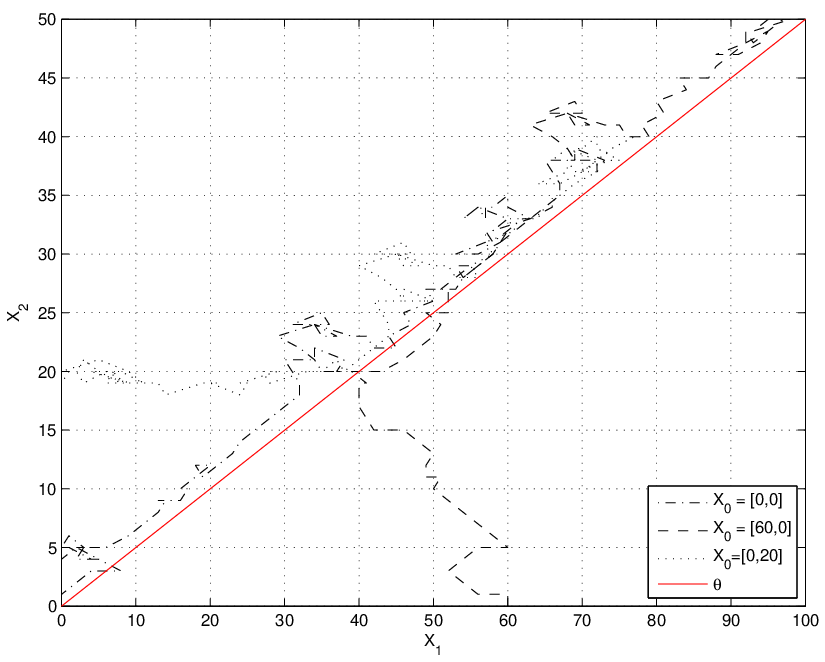
We consider how the workload vector grows for various initial conditions:
| (5.2) |
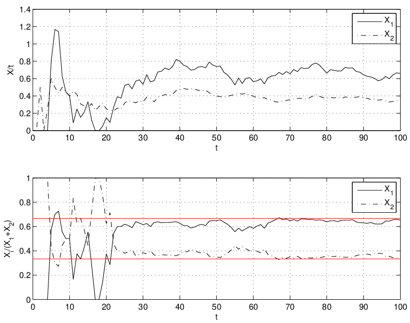
In Figure 4(a), we plot the trajectories of for the different initial conditions, along with the line . We can see that all three trajectories converge to the desired fairness vector . In Figure 4(b), we see the scaled backlogs, , and the relative backlog, , converge starting from initial condition . Moreover, we see that they quickly achieve the fairness criterion which is shown in red.
When there are service vectors, there are subsets of service vectors and corresponding boundary vectors which satisfy (4.30).
| (5.3) |
Now there are two boundary vectors of interest: the one between and as well as the one between and . The boundary which matters depends on as described in Section 4.3. From that discussion, we know that and are the necessary MaxWeight matrices to move the boundary vectors between and and between and , respectively, to fairness direction . We refer to as the necessary MaxWeight Matrix to achieve fairness direction , given system load, . Let ; we use as before and we can achieve the desired fairness criterion. On the other hand, if , will not achieve the desired fairness criterion, but matrix will. Hence:
| (5.4) |
We can see in Figure 5 how the asymptotic dynamics of the queues depend on and . The fairness criterion is shown in red.

In the next experiment, we consider a system with queues and service vectors. Again there is only one boundary vector to consider. As long as the fairness direction is feasible there is only one MaxWeight matrix (to a scale factor) to achieve it. Feasibility depends on .
| (5.5) |
The desired fairness criterion is
| (5.6) |
With some algebra, it is easy to see that as long as the load vector is such that the fairness direction is feasible, then the necessary MaxWeight matrix, , to achieve it is as follows:
| (5.7) |
The system load oscillates between being stable and unstable. Hence, there are temporary periods of overload.
| (5.8) |
The system spends 500 time slots in the stable mode––then switches to spend 500 time slots in the unstable mode–. Arrivals to queue in each time slot are uniformly distributed between . When the system is in the stable mode, MaxWeight Scheduling should stablize the workload. When it is in the unstable mode, MaxWeight Scheduling should achieve the desired fairness criterion.
Figure 6 plots the scaled workload, , under this unstable/stable system. We can see that for the first unstable period (), the fairness criterion is quickly achieved. However, on the next unstable period, the scaled backlogs () do not appear to stabilize within the epoch period. This is because the workload has been stablized during the stable period and we are scaling by the total time, not just the time starting from when we enter the period of instability. Hence, it may actually take a very long time before the scaled backlogs converge. One the other hand, the fairness criteria is quickly achieved. The third subfigure shows how the backlogs grow relative to each other: . We can see in this figure, the fairness criterion is achieved very quickly (plotted in red) during unstable periods. During stable periods this relative backlog is not very informative since all the backlogs will grow to zero.

While our fairness results for controlling the backlog were asymptotic, these numerical results suggest that the fairness criterion can be achieved very rapidly.
6 Discussion and Conclusion
In many real world systems, traffic load is unpredictable and often bursty in nature. In any finite window of time, the system may enter a period of temporary instability where the rate of incoming jobs is larger than the rate at which jobs can be serviced. During such periods of stress, it is natural to want to allocate limited service resources across various jobs classes in a fair manner.
In this work, we consider how to fairly serve under-provisioned queues. We focus on MaxWeight Scheduling policies because they are simple to implement and behave well during stable periods. In particular, MaxWeight policies guarantee finite backlogs when the system load is within the stability region. We find that, whenever the system is overloaded, the backlog approaches a straight line as the time window during which the system is overloaded increases. This straight line can be characterized as a fixed point, or equivalently, as the solution to a simple convex program. As such, it is straightforward to identify this line, as a function of the system parameters, the load vector , and the MaxWeight matrix .
Considering a fair allocation of resources in overloaded systems to be such that the backlog grows along a certain direction , we show how to choose the MaxWeight matrix to guarantee that the backlog will indeed grow along this direction, as long as this direction is feasible. Additionally, MaxWeight is shown to asymptotically minimize the backlog, among all other policies that achieve the same fairness criterion. As it turns out the choice of is robust with respect to the load vector in the sense that for every direction , there exists a partition of the instability region into subsets, such that the same matrix will work for all load vectors in the same subset. In particular, it is sufficient to know what subset belongs to, and it is unnecessary to know the exact value of . Via numerical simulations we see that MaxWeight scheduling policy performs as expected; it achieves the fairness criterion during periods of overload and it stabilizes the queues otherwise.
Our analysis relies on geometrical arguments that are applied directly to individual backlog traces. In particular, no probabilistic assumptions are made. The only necessary assumption is that the arriving workload has a well defined long run average. This approach is also helpful in developing intuition with respect to the system dynamics.
This work can be extended in various directions. As demonstrated in Section 4.1.2, there exist some fairness criteria that are infeasible via MaxWeight Matching. So, one might consider whether other policies, such as Projective Cone Scheduling from Ross and Bambos (2009), would expand the set of feasible fairness criteria. In a similar vein, one might want to obtain other fairness criteria for unstable systems. Third, it may be possible to extend this work to networks of parallel queueing systems, by relying on results from Shah and Wischik (2011). Finally, while we have established convergence of the backlog vector under vary mild traffic conditions, if more restrictive assumptions are made (such as Markovian queues) one might be able to obtain results on the rate of convergence as well.
In this work we take a different view to traditional queueing. Namely, we focus on the instability region. While it is certainly desirable to operate systems within the stability region, there are many real world scenarios where this may not be possible. Input traffic may surge due to unplanned circumstances. Service resources may be reduced due to unavoidable accidents or catastrophes. During these periods of temporary instability it is often necessary to allocate limited resources in a fair manner. Once the system exits the window of stress, it will be stabilizable and the natural goals of throughput maximization and cost minimization can be restored.
References
- Armony and Bambos (2003) Armony, M., N. Bambos. 2003. Queueing dynamics and maximal throughput scheduling in switched processing systems. Queueing Systems 44 209–252.
- Bonald et al. (2006) Bonald, T., L. Massoulie, A. Proutiere, J. Virtamo. 2006. A queueing analysis of max-min fairness, proportional fairness and balanced fairness. Queueing Systems 53 65–84.
- Boyd and Vandenberghe (2004) Boyd, S., L. Vandenberghe. 2004. Convex Optimization. Cambridge University Press.
- Eryilmaz and Srikant (2005) Eryilmaz, A., R. Srikant. 2005. Fair resource allocation in wireless networks using queue-length-based scheduling and congestion control. IEEE Infocom.
- Eryilmaz and Srikant (2006) Eryilmaz, A., R. Srikant. 2006. Joint congestion control, routing, and mac for stability and fairness in wireless networks. IEEE Journal on Selected Areas in Communications 24 1514–1524.
- Georgiadis and Tassiulas (2006) Georgiadis, Leonidas, Leandros Tassiulas. 2006. Optimal overload response in sensor networks. IEEE Transactions on Information Theory 52 2684–2696.
- Kelly et al. (1998) Kelly, F. P., A.K. Maulloo, D.K.H. Tan. 1998. Rate control in communication networks: shadow prices, proportional fairness and stability. Journal of the Operational Research Society 49 237–252.
- Kelly and Williams (2004) Kelly, F. P., R. J. Williams. 2004. Fluid model for a network operating under a fair bandwidth-sharing policy. Annals of Applied Probability 14 1055–1083.
- Loynes (1963) Loynes, R.M. 1963. The stability of a queue with non-independent interarrival and service times. Proceedings of the Cambridge Philisophical Society 58 497–530.
- Mandelbaum and Stolyar (2004) Mandelbaum, A., S. Stolyar. 2004. Scheduling flexible servers with convex delay costs: Heavy-traffic optimality of the generalized c-rule. Operations Research 52(6) 836–855.
- Massoulie (2007) Massoulie, L. 2007. Structural properties of proportional fairness: Stability and insensitivity. Annals of Applied Probability 17 809–839.
- Mazumdar et al. (1991) Mazumdar, R., L. Mason, C. Douligeris. 1991. Fairness in network optimal flow control: optimality of product forms. IEEE Transactions on Communications 39 775–782.
- McKeown et al. (1999) McKeown, N., A. Mekkittikul, V. Anantharam, J. Walrand. 1999. Achieving 100 throughput in an input-queued switch. IEEE Transactions on Communications 47 1260–1267.
- Mo and Walrand (2000) Mo, J., J. Walrand. 2000. Fair end-to-end window-based congestion control. IEEE/ACM Transactions on Networking 8 556–567.
- Neely (2006) Neely, M. J. 2006. Super-fast delay tradeoffs for utility optimal fair scheduling in wireless networks. IEEE Journal on Selected Areas in Communications 24 1489–1501.
- Neely et al. (2005) Neely, M. J., E. Modiano, C. Li. 2005. Fairness and optimal stochastic control for heterogeneous networks. IEEE Infocom.
- Perry and Whitt (2009) Perry, O., W. Whitt. 2009. Responding to unexpected overloads in large-scale service systems. Management Science 55 1353–1367.
- Perry and Whitt (2011) Perry, O., W. Whitt. 2011. A fluid approximation for service systems responding to unexpected overloads. Operations Research to appear.
- Ross and Bambos (2009) Ross, K., N. Bambos. 2009. Projective cone scheduling (PCS) algorithms for packet switches of maximal throughput. IEEE/ACM Transactions on Networking 17(3) 976–989.
- Shah and Wischik (2011) Shah, D., D. Wischik. 2011. Fluid models of switched networks in overload Working paper.
- Stolyar (2004) Stolyar, S. 2004. Maxweight scheduling in a generalized switch: State space collapse and workload minimization in heavy traffic. The Annals of Applied Probability 14(1) 1–53.
- Tassiulas (1995) Tassiulas, L. 1995. Adaptive back-pressure congestion control based on local information. IEEE Transactions on Automatic Control 40 236–250.
- Tassiulas and Bhattacharya (2000) Tassiulas, L., P.P. Bhattacharya. 2000. Allocation of interdependent resources for maximal throughput. Stochastic Models 16 27 – 48.
- Tassiulas and Ephremides (1992) Tassiulas, L., A. Ephremides. 1992. Stability properties of constrained queueing systems and scheduling policies for maximum throughput in multihop radio networks. IEEE Transactions on Automatic Control 37 1936–1948.
Proof of Lemma 3.2:
We write (using similar arguments like in equations of A.22 to A.27 of Ross and Bambos (2009)),
| (.1) | |||||
To see the above steps, recall the following. First, for every and any , by assumption. Therefore, , hence, from (3.15) we get for with , for every and any . Moreover, , hence, from (3.13) we get , for all and any .
Proof of Lemma 3.3:
Note that eventually (for any large ), expand the terms as follows:
| (.2) |
and observe that letting we get
| (.3) |
since . This completes the proof of the lemma.
Proof of Lemma 3.4: We write
| (.4) |
and observe that for every , hence, . Therefore, since is diagonal (with positive elements), we have . Projecting on we get
| (.5) |
Dividing by and letting , we get
| (.6) |
This completes the proof of the lemma.
Proof of Lemma 3.5: Indeed (recalling that is positive-definite), we have
| (.7) | |||||
so . But since , we must have , therefore, , which implies . This completes the proof of the lemma.
Proof of Lemma 3.6: Rewrite the inequality as , since . This is equivalent (since ) to
| (.8) |
But this is true by Lemma 3.4 applied to the sequence with . This complete the proof of the lemma.
Proof of Lemma 3.7: We have 2 cases to show since, by definition of we have that . The first case is A) and the second is B) .
A) We first show that . We start by showing that there is no increasing unbounded subsequence of such that , where . Note that this also implies that . Arguing by contradiction, suppose it exists. Observe that for every we have
| (.9) |
where is the maximum workload that can arrive in queue in any time slot (see model in Ross and Bambos (2009) for assumption of boundedness) and is the maximum workload that can be removed from queue in any time slot. Dividing by , letting , we get
| (.10) |
which implies that and establishes the desired contradiction.
B) We still need to show that . Arguing by contradiction, suppose there exists a subsequence of (and corresponding subsequence of ) such that , hence, . Applying Lemmas 3.2 and 3.3 with
| (.11) |
It follows that
| (.12) | |||||
Now applying Lemma 3.4 on the subsequence with we get
| (.13) |
using (.12). Hence, , which implies by Lemma 3.5. But this is impossible since by definition of subsequence , , which completes the proof of the lemma.
Proof of Lemma 3.8: Consider a subsequence such that for each :
| (.14) |
Note that by definition: and . Further, because , there exist and , such that for all ; hence, MaxWeight Scheduling policies will never idle for and .
We have for such that :
| (.15) | |||||
Where such that for all , . It’s existence is given by Proposition 3.1. For such that , we have:
| (.16) | |||||
Which means that and
| (.17) |
which gives us that .
Finally, we have to show that if , then . We have seen that is the proportion of time that service vector is used under MaxWeight Scheduling once for all . By Proposition 3.1, we know that exists. By contradiction, suppose that . This implies that there exists such that . Since , we must use for some . This contradicts the definition of , which by (3.13) says that MaxWeight Scheduling would use rather than which would imply that . Hence, if , .
Proof of Lemma 3.9: This follows from Lemma 3.8. Replacing we have
| (.18) | |||||
where the last equality follows from the fact that is a fixed point.
Proof of Lemma 3.10: This result follows from the KKT conditions for optimality of the convex program (3.9). Our goal is to show that if is such that for all with , we have that , then it is a solution to the convex program (3.9). The KKT conditions are necessary and sufficient for optimality if the objective function is differentiable and Slater’s constraint is satisfied Boyd and Vandenberghe (2004). Our objective function is clearly differentiable.
Slater’s condition says that there exists such that , , and . It is clear that satisfies this condition. Since the KKT conditions are necessary and sufficient in this case and there is only one solution, it will follow that there is exactly one fixed point if all fixed points satisfy the KKT conditions.
To examine the KKT conditions, we first rewrite the convex program in (3.9) as an equivalent convex program:
| (.19) | |||||
Let (and correspondingly ) be the solution to the preceding convex program. The KKT conditions for optimality say that all the constraints must be satisfied and:
| (.20) |
We look at the first condition:
| (.21) | |||||
Now we show that for any fixed point, there exists which satisfy the KKT condition (.20). To do this, suppose we are given a fixed point with
| (.22) |
We will construct non-negative Lagrange multiplies to satisfy the KKT conditions.
Consider such that . In order to satisfy the third constraint in (.20), . Now if , in order to satisfy the first constraint in (.21) we have that . To ensure that the Lagrange multipliers are non-negative, we must have that for all . Subsequently:
| (.23) |
Consider . To satisfy the fourth constraint in (.20), . Now to satisfy the second constraint in (.21):
| (.24) |
which also satisfies the non-negativity of . Consider and . By the assumption that is a fixed point:
| (.25) | |||||
Hence, we can satisfy the KKT conditions in (.20) with non-negative . Since any fixed point satisfies the necessary and sufficient KKT conditions, all fixed points are solutions to the convex program. There is only one solution and so there is only one fixed point.
Proof of Lemma 4.1: We show this via construction. Recall that is diagonal: . For
| (.26) |
where the positivity comes from the fact that each element is positive. If ,
| (.27) |
or some other arbitrary positive value.
Now, for any () and the following holds:
| (.28) | |||||
Proof of Proposition 4.1: Assume that Conditions 1 and 2 are satisfied. We show this implies there exists a such that . We first consider Condition 2. This says that is the boundary of cones where defined by . By Lemma 4.1, we can construct a such that for all :
| (.29) |
Now, in conjunction with Condition 1, we have that is a fixed point. By Theorem 3.1, we have that
| (.30) |
Now suppose there exists a such that . By Theorem 3.1, is a (the only) fixed point and, hence, satisfies Condition 1. Now, we show that Condition 2 is satisfied by constructing the necessary . Similar to the construction of in the proof of Lemma 4.1 we can determine –the boundary induced when . That is:
| (.31) |
which equals if and only if . This satisfies Condition 2.
Proof of Theorem 4.1: The proof is via contradiction. Since both MaxWeight Scheduling and this alternative algorithm achieve the fairness criterion, there exists some such that . Let’s assume that is not the smallest scaled workload that achieves the fairness criterion so that .
Since
| (.32) |
for any , there exists such that for all :
| (.33) |
For any such that , there exists some such that for all , and so after time , , where and are the departures and service vector used in time slot as defined in Section 2. Given , there exists such that:
| (.34) |
Define be defined as:
| (.35) |
Note that . is the proportion of time service vector is used up to time . If the limit in (.35) does not exists, we can take a sub-limit which is well-defined since .