Renormalized waves and thermalization of the Klein-Gordon equation: What sound does a nonlinear string make?

Although we study the wave system (4) for strongly interacting waves, to motivate the introduction of renormalized waves, we first address (4) in the linear case, followed by the case of weakly interacting waves. In the absence of nonlinearity, $\lambda=0$, (4) reduces to the linear KG equation. Hence, wave solutions decouple into linearly independent Fourier modes, with conservation of energy in each mode. Specifically, the Fourier series for $p(x,t)$ and $u(x,t)$ are

	$\displaystyle p(x,t)$	$\displaystyle=$	$\displaystyle\frac{1}{\sqrt{2\pi}}\sum_{k}p_{k}(t)e^{-\imath kx},$
	$\displaystyle u(x,t)$	$\displaystyle=$	$\displaystyle\frac{1}{\sqrt{2\pi}}\sum_{k}u_{k}(t)e^{-\imath kx}$

with summation $k$ over all integer values. Taking $p(x,t)$ and $u(x,t)$ as real fields restricts $u_{k}=u_{-k}^{*}$ and $p_{k}=p_{-k}^{*}$ so that $H$ becomes

	$\displaystyle H$	$\displaystyle=$	$\displaystyle\sum_{k}E_{k},$		(6)
	$\displaystyle E_{k}$	$\displaystyle=$	$\displaystyle\frac{1}{2}(|p_{k}|^{2}+\omega_{k}^{2}|u_{k}|^{2}).$		(7)

Here $E_{k}$ is the linear energy in mode $k$, while $\omega_{k}^{2}=1+k^{2}$ is the linear dispersion relation. In addition to constructing Fourier mode solutions, one may also make a secondary transformation to study the kinetics of interacting waves

$$a_{k}=\frac{p_{k}-\imath\omega_{k}u_{k}}{\sqrt{2\omega_{k}}}.$$

(8)

In this new basis, the equations of motion become

$$\imath\dot{a_{k}}=\frac{\partial}{\partial a_{k}^{*}}H(a_{k},a_{k}^{*}),$$

(9)

where the Hamiltonian, $H(a_{k},a_{k}^{*})$ also acquires a convenient form:

$\displaystyle H$

$\displaystyle=$

$\displaystyle\sum_{k}\omega_{k}|a_{k}|^{2}.$

(10)

With the dynamic equations written in the variables $a_{k}$, the linear oscillator solutions take the form $a_{k}(t)=A_{k}e^{-\imath\omega_{k}t}$, where the amplitude and phase are contained in the complex variable $A_{k}$. As a result, each wave number oscillates with a negative frequency so that the Fourier transform of a linear wave is a Dirac $\delta$ function

	$\displaystyle\widehat{a}_{k}(\omega)$	$\displaystyle=$	$\displaystyle\frac{1}{\sqrt{2\pi}}\int_{-\infty}^{\infty}a_{k}(t)e^{-\imath\omega t}\,\mathrm{d}t$		(11)
		$\displaystyle=$	$\displaystyle A_{k}\delta(\omega_{k}+\omega).$		(12)

Secondly, the infinite time correlation of any two linear waves, including the case of $k=\pm l$, vanish:

$$\langle a_{k}a_{l}\rangle=0.$$

(13)

Hence, linear solutions are uncorrelated waves, which oscillate at a single frequency.

In the presence of nonlinearity, $\lambda>0$, the waves $a_{k}$ no longer decouple into linear oscillators and therefore no longer conserve the energy $E_{k}$. For instance, the wave amplitudes $|a_{k}(t)|$ do not remain constant but fluctuate from the nonlinear interaction. As a result, we seek to characterize the nonlinear effect on both the amplitude and phase behavior of the waves $a_{k}$. Before proceeding to the case of strongly interacting waves, we first examine the case of a weak nonlinearity. By weak nonlinearity we mean the maximum amplitude of $u$ is order $1$, while the coupling strength remains small $\lambda\ll 1$. Moreover, with the onset of nonlinearity, especially in the presence of strong interactions, the waves $a_{k}$ no longer exhibit the linear properties (12) and (13). We therefore follow the ideas of Gershgorin et al. [12] and introduce renormalized waves $c_{k}$ in lieu of (8). Renormalized waves form a useful basis since they exhibit characteristics of linear waves. Namely, renormalized waves have vanishing correlators and approximately oscillate with a single frequency. In analogy with the linear waves (8), renormalized waves are defined through a linear combination of the Fourier transforms $u_{k}$ and $p_{k}$, however, linear frequencies are altered to renormalized frequencies:

$$c_{k}=\frac{1}{\sqrt{2\tilde{\omega}_{k}}}(p_{k}-\imath\tilde{\omega}_{k}u_{k}).$$

(14)

The transformation to renormalized waves is canonical (up to a factor of $\imath$) provided the yet to be determined frequencies satisfy $\tilde{\omega}_{k}>0$ and $\tilde{\omega}_{k}=\tilde{\omega}_{-k}$.

We now examine the evolution of renormalized waves in the presence of a weak nonlinearity $\lambda\ll 1$ through a perturbation expansion. Specifically, we show that the standard procedure of choosing renormalized frequencies to eliminate resonant terms yields the same result as choosing frequencies to enforce a vanishing correlator for waves at $\pm k$ wave numbers, i.e., $\langle c_{k}c_{-k}\rangle$. Written in terms of renormalized waves, the dynamic equations for $c_{k}$ are

	$\displaystyle\imath\dot{c}_{k}$	$\displaystyle=$	$\displaystyle\frac{\partial H(c_{k},c_{k}^{*})}{\partial c_{k}^{*}}$		(15)
	$\displaystyle\imath\dot{c}_{k}$	$\displaystyle=$	$\displaystyle\frac{\tilde{\omega}_{k}}{2}\Big[(1+\frac{\omega_{k}^{2}}{\tilde{\omega}_{k}^{2}})c_{k}+(1-\frac{\omega_{k}^{2}}{\tilde{\omega}_{k}^{2}})c_{-k}^{*}\Big]$		(16)
		$\displaystyle+$	$\displaystyle\lambda\sum_{l,m,n}T_{klmn}\Big[4c_{l}^{*}c_{m}^{*}c_{n}^{*}\delta_{k+l+m+n}$
		$\displaystyle-$	$\displaystyle 12c_{l}c_{m}^{*}c_{n}^{*}\delta_{l-k-m-n}-4c_{l}c_{m}c_{n}\delta_{k-l-m-n}$
		$\displaystyle+$	$\displaystyle 12c_{n}c_{m}c_{l}^{*}\delta_{l+k-m-n}\Big],$
	$\displaystyle T_{klmn}$	$\displaystyle=$	$\displaystyle\frac{1}{32\pi(\tilde{\omega}_{k}\tilde{\omega}_{l}\tilde{\omega}_{m}\tilde{\omega}_{n})^{\frac{1}{2}}},$

where $T_{klmn}$ is the series coefficient, and $\delta_{x}=1$ when $x=0$ and $\delta_{x}=0$ otherwise. The summation is over all integers $l,m,n$. As is commonly the case in kinetic theories, wave behavior is dominated by interacting resonant terms, for instance, those which force the order-one linear oscillators $c_{k}$ on resonance. The nonlinear term in (15) admits only one such resonance, which comes from the term $c_{n}c_{m}c_{l}^{*}=|c_{n}|^{2}c_{k}$ when $k=n,m=l$ or $k=m,n=l$. The presence of only one resonant term follows from the fact that the linear dispersion relation $\omega_{k}^{2}=1+k^{2}$ is concave up [16]. For instance, the harmonics generated by the products $c_{l}^{*}c_{m}^{*}c_{n}^{*}$, $c_{l}c_{m}^{*}c_{n}^{*}$, and $c_{l}c_{m}c_{n}$ cannot oscillate with frequency $\tilde{\omega}_{k}$ provided $\tilde{\omega}_{k}$ is a concave function of $k$.

In addition to each resonant term in the series $c_{n}c_{m}c_{l}^{*}$, there is an equivalent term in $c_{l}c_{m}^{*}c_{n}^{*}$ containing the variable $c_{-k}^{*}$ when $n=-k,l=m$ or $m=-k,l=n$. We now remove both the resonant terms and their equivalent $c_{-k}^{*}$ terms from the nonlinear series, and absorb them into the coefficients of $c_{k}$ and $c_{-k}^{*}$. We do this so that upon seeking a small amplitude ($\lambda\ll 1$) solution, we may simultaneous handle both the zeroth, $O(1)$, and first order, $O(\lambda)$, corrections to the renormalized frequencies. The dynamic equations then become:

	$\displaystyle\imath\dot{c}_{k}$	$\displaystyle=$	$\displaystyle g_{k}(t)c_{k}+h_{k}(t)c_{-k}^{*}+\lambda r_{k}(t),$		(17)
	$\displaystyle g_{k}(t)$	$\displaystyle=$	$\displaystyle\frac{\tilde{\omega}_{k}}{2}\Big(1+\frac{\omega_{k}^{2}}{\tilde{\omega}_{k}^{2}}\Big)+\lambda\mu_{k}(t),$
	$\displaystyle h_{k}(t)$	$\displaystyle=$	$\displaystyle\frac{\tilde{\omega}_{k}}{2}\Big(1-\frac{\omega_{k}^{2}}{\tilde{\omega}_{k}^{2}}\Big)-\lambda\mu_{k}(t),$
	$\displaystyle\mu_{k}(t)$	$\displaystyle=$	$\displaystyle 24\sum_{m}T_{mmkk}|c_{m}|^{2}-12T_{kkkk}|c_{k}|^{2},$
	$\displaystyle r_{k}(t)$	$\displaystyle=$	$\displaystyle\sum_{l,m,n}^{\prime}T_{klmn}\Big[4c_{l}^{*}c_{m}^{*}c_{n}^{*}\delta_{k+l+m+n}$
		$\displaystyle-$	$\displaystyle 12c_{l}c_{m}^{*}c_{n}^{*}\delta_{l-k-m-n}-4c_{l}c_{m}c_{n}\delta_{k-l-m-n}$
		$\displaystyle+$	$\displaystyle 12c_{n}c_{m}c_{l}^{*}\delta_{l+k-m-n}\Big].$

Here the prime in $r_{k}$ restricts the summation to exclude all resonant terms having either $c_{k}$ or their equivalent terms containing $c_{-k}^{*}$. Meanwhile, the time dependent coefficients $g(t)$ and $h(t)$ are related by

$\displaystyle g_{k}(t)+h_{k}(t)$

$\displaystyle=$

$\displaystyle\tilde{\omega}_{k}.$

(18)

Thus far, Eq. (17) is exact.

We now extract approximate solutions to (17), in the limit $\lambda\ll 1$, for the initial value problem:

$\displaystyle c_{k}(0)=C_{k}.$

(19)

To remain consistent in the small amplitude approximation, we assume the initial field is small with finite energy. Hence, each $C_{k}<1$ while $C_{k}\rightarrow 0$ as $k\rightarrow\infty$. To obtain a solution, we seek an asymptotic series for $c_{k}$ in powers of $\lambda$ with a single frequency leading term:

$\displaystyle c_{k}(t)$

$\displaystyle=$

$\displaystyle C_{k}e^{-\imath\tilde{\omega}_{k}t}+\lambda c_{k}^{(1)}(t)+\lambda^{2}c_{k}^{(2)}(t)+\ldots.$

(20)

In general, even at zeroth order in $\lambda$, an arbitrary choice of $\tilde{\omega}_{k}$ will couple solutions $c_{\pm k}$ together through the coefficients $g(t)$ and $h(t)$. As a result, the proposed ansatz (20) requires the following two consistency conditions on $\tilde{\omega}_{k}$:

	$\displaystyle g_{k}$	$\displaystyle=$	$\displaystyle\tilde{\omega}_{k},$		(21)
	$\displaystyle h_{k}$	$\displaystyle=$	$\displaystyle 0.$		(22)

The first consistency condition (21) comes from the fact that we have chosen $c_{k}$ to oscillate with frequency $\tilde{\omega}_{k}$. Meanwhile, the second condition (22) follows from the fact that our ansatz has no dependence on the initial value $C_{-k}$, or equivalently that $c_{k}$ decouples from $c_{-k}$. Relation (18) however, implies the equivalence of the two conditions (21), (22). Therefore, choosing $\tilde{\omega}$ through (21) as the $c_{k}$ oscillator single frequency automatically guarantees (22), thereby decoupling the fields $c_{k}$ and $c_{-k}^{*}$. Using Eq. (21) to extract the expression for $\tilde{\omega}_{k}$ yields

	$\displaystyle\tilde{\omega}_{k}$	$\displaystyle=$	$\displaystyle\frac{\tilde{\omega}_{k}}{2}\Big(1+\frac{\omega_{k}^{2}}{\tilde{\omega}_{k}^{2}}\Big)+\lambda\mu_{k}^{(0)}+O(\lambda^{2}),$		(23)
	$\displaystyle\mu_{k}^{(0)}$	$\displaystyle=$	$\displaystyle 24\sum_{m}T_{mmkk}|C_{m}|^{2}-12T_{kkkk}|C_{k}|^{2}.$		(24)

To solve for $\tilde{\omega}_{k}$ to $O(\lambda^{2})$, we assume the amplitude in a single mode is much smaller than the total averaged wave field. Therefore, neglecting the term $T_{kkkk}|C_{k}|^{2}$ results in

	$\displaystyle\tilde{\omega}_{k}^{2}$	$\displaystyle=$	$\displaystyle\omega_{k}^{2}+3\lambda\langle S\rangle+O(\lambda^{2})$		(25)
		$\displaystyle=$	$\displaystyle 1+3\lambda\langle S\rangle+k^{2}+O(\lambda^{2}).$		(26)

Here we have made use of the fact that $\mu_{k}^{0}$ is proportional to the time-averaged value of the wave field

	$\displaystyle\langle S(t)\rangle$	$\displaystyle=$	$\displaystyle\langle\frac{1}{2\pi}\int_{0}^{2\pi}u^{2}(x,t)\,\mathrm{d}x\rangle$		(27)
		$\displaystyle=$	$\displaystyle\sum_{m}\frac{1}{4\pi\tilde{\omega}_{m}}(|C_{-m}|^{2}+|C_{m}|^{2}).$		(28)

Note that within the framework of the small amplitude ansatz, the approximation (25) only remains valid over time scales $O(\lambda^{-2})$. As a result, to remain consistent, the time average taken in (27) should be made over, at most, comparable time scales, $O(\lambda^{-2})$.

With the values of $\tilde{\omega}_{k}$ solved to $O(\lambda)$, we may substitute $c_{k}^{(0)}=C_{k}e^{-\imath\tilde{\omega}_{k}t}$ into the nonlinear term $r(t)$ and solve for the first-order contribution to $c_{k}(t)$. Consequently, $c_{k}^{(1)}(t)$ satisfies the equation

	$\displaystyle\imath\dot{c}_{k}^{(1)}$	$\displaystyle=$	$\displaystyle\tilde{\omega}_{k}c_{k}^{(1)}+r_{k}^{(0)}(t),$		(29)
	$\displaystyle c_{k}^{(1)}(0)$	$\displaystyle=$	$\displaystyle 0.$		(30)

Here $r_{k}^{(0)}(t)$ is the nonlinear term $r(t)$ evaluated using $c_{k}^{(0)}=C_{k}e^{-\imath\tilde{\omega}_{k}t}$. Equation (29) therefore describes a first-order linear oscillator forced off resonance by $r_{k}^{(0)}(t)$. The solution for $c_{k}^{(1)}(t)$ is

	$\displaystyle c_{k}^{(1)}(t)$	$\displaystyle=$	$\displaystyle-\sum_{l,m,n}^{\prime}T_{klmn}\Big[\frac{4C_{l}^{*}C_{m}^{*}C_{n}^{*}e^{\imath(\tilde{\omega}_{l}+\tilde{\omega}_{m}+\tilde{\omega}_{n})t}}{\tilde{\omega}_{k}+\tilde{\omega}_{l}+\tilde{\omega}_{m}+\tilde{\omega}_{n}}\delta_{k+l+m+n}$		(31)
		$\displaystyle-$	$\displaystyle\frac{12C_{l}C_{m}^{*}C_{n}^{*}e^{\imath(-\tilde{\omega}_{l}+\tilde{\omega}_{m}+\tilde{\omega}_{n})t}}{\tilde{\omega}_{k}-\tilde{\omega}_{l}+\tilde{\omega}_{m}+\tilde{\omega}_{n}}\delta_{l-k-m-n}$
		$\displaystyle-$	$\displaystyle\frac{4C_{l}C_{m}C_{n}e^{-\imath(\tilde{\omega}_{l}+\tilde{\omega}_{m}+\tilde{\omega}_{n})t}}{\tilde{\omega}_{k}-\tilde{\omega}_{l}-\tilde{\omega}_{m}-\tilde{\omega}_{n}}\delta_{k-l-m-n}$
		$\displaystyle+$	$\displaystyle\frac{12C_{n}C_{m}C_{l}^{*}e^{\imath(\tilde{\omega}_{l}-\tilde{\omega}_{m}-\tilde{\omega}_{n})t}}{\tilde{\omega}_{k}+\tilde{\omega}_{l}-\tilde{\omega}_{m}-\tilde{\omega}_{n}}\delta_{l+k-m-n}\Big]$
		$\displaystyle+$	$\displaystyle De^{-\imath\tilde{\omega}_{k}t}.$

In the solution for $c_{k}^{(1)}$, the prime in the summation indicates that there are no terms oscillating with frequencies $\pm\tilde{\omega}_{k}$. This follows from the fact that we have removed the terms in $r(t)$ oscillating at frequencies $\pm\tilde{\omega}_{k}$. Meanwhile, the constant $D$, from the homogeneous term, is chosen to satisfy the initial value $c_{k}^{(1)}(0)=0$. With the asymptotic solution (20) solved to $O(\lambda^{2})$, we may calculate the time averaged correlator, $\langle c_{k}c_{-k}\rangle$, for waves $\pm k$:

	$\displaystyle\langle c_{k}c_{-k}\rangle$	$\displaystyle=$	$\displaystyle C_{k}C_{-k}\langle e^{-\imath 2\tilde{\omega}_{k}t}\rangle+\lambda C_{k}\langle e^{-\imath\tilde{\omega}_{k}t}c_{-k}^{(1)}\rangle$		(32)
		$\displaystyle+$	$\displaystyle\lambda C_{-k}\langle e^{-\imath\tilde{\omega}_{k}t}c_{k}^{(1)}\rangle+O(\lambda^{2}).$		(33)

Using formula (1) with an averaging time of $O(\lambda^{2})$ will result in $\langle e^{-\imath 2\tilde{\omega}_{k}t}\rangle=O(\lambda^{2})$. Meanwhile, the long time average $\langle e^{-\imath\tilde{\omega}_{k}t}c_{-k}^{(1)}\rangle$ picks out the component of $c_{-k}^{(1)}$ with frequency $\tilde{\omega}_{k}$. Since $c_{\pm k}^{(1)}(t)$ contains no term oscillating at frequency $\tilde{\omega}_{k}$, taking a time average over length $O(\lambda^{-2})$ will also tend this term to zero:

$\displaystyle\langle c_{k}c_{-k}\rangle$

$\displaystyle=$

$\displaystyle O(\lambda^{2}).$

(34)

Therefore, to first order in $\lambda$, choosing the renormalized frequencies $\tilde{\omega}_{k}$ to remove the resonant terms in (15) is equivalent to choosing them to enforce a vanishing correlator.

In studying LTE solutions, we are specifically interested in the case of strongly interacting waves, $\lambda\gg 1$. Even in the presence of a strong nonlinearity, one may introduce renormalized waves defined by (14). Extending the properties of linear waves, the new renormalized frequencies $\tilde{\omega}$ are then found by imposing that waves $c_{k}$ and $c_{-k}$ remain uncoupled and their correlations vanish [12, 13]:

$\displaystyle\langle c_{k}c_{-k}\rangle$

$\displaystyle=$

$\displaystyle 0.$

(35)

If one has a KG solution $u(x,t)$ for some long time interval, substituting the definition of $c_{k}$ into (35) yields an expression for $\tilde{\omega}_{k}$:

$\displaystyle\tilde{\omega}_{k}^{2}=\frac{\langle|p_{k}|^{2}\rangle}{\langle|u_{k}|^{2}\rangle}.$

(36)

Equation (36) provides a useful formula for numerically obtaining the renormalized frequencies. Despite the fact that the renormalized transformation defined by Eqs. (14) and (36) is always mathematically possible, there is no guarantee that the waves $c_{k}$ stand out as a useful coordinate system. The waves $c_{k}$ do however form a useful basis provided the Fourier modes $u_{k}$ exhibit narrow band single frequency oscillations. When $u_{k}$ does oscillate with roughly one frequency, the formula (36) identifies $\tilde{\omega}_{k}$ with the frequency of oscillation. In the case of the KG equation with a strong $u^{4}$ interaction, we do in fact find that the waves $c_{k}$ form narrow band oscillators with a central frequency $\tilde{\omega}_{k}$. We verify these wave properties in our numerical experiments, implying renormalized waves are a natural basis to study the LTE spectra. We demonstrate in our numerical experiments that in the limit $\lambda\gg 1$, the renormalized frequencies are very well approximated by the dispersion relation

$\displaystyle\tilde{\omega}_{k}^{2}\approx 1+2.59\lambda\langle S\rangle+k^{2}.$

(37)

Here we refer to $2.59\lambda\langle S\rangle=\tilde{\omega}_{k}^{2}-\omega_{k}^{2}$ as the mass shift.

In the case of large $\lambda$, the nonlinear time scale may be estimated by comparing the size of terms in the KG equation. Specifically, assuming the field $u(x,t)$ is order one, the time derivative will balance the nonlinear term, $u_{tt}\sim\lambda u^{3}$, provided that the characteristic nonlinear timescale $\tau_{0}\sim\lambda^{-1/2}$. Note that this estimate only holds for large $\lambda$, or when $\lambda$ dominates the linear dispersive term in the KG equation. In our numeric experiments, we find that LTE solutions exhibit $O(\lambda^{-1/2})$ as the natural fundamental period, while earlier work focusing on the analytic development of short time KG solutions [17] further verifies $\lambda^{-1/2}$ as the strong amplitude time scale. Consequently, we define LTE time-averaged quantities $\langle A\rangle$ over many periods of the time scale $\tau_{0}$:

$$\langle A\rangle(t)=\lim_{\Delta T\gg\tau_{0}}\frac{1}{\Delta T}\int_{t-\Delta T/2}^{t+\Delta T/2}A(t^{\prime})\,\mathrm{d}t^{\prime}.$$

(38)

Our numeric experiments try to capture solution properties at large wave numbers, especially within the exponential decay of the spectrum. We therefore use a pseudospectral method to maintain high numeric accuracy in both space and time. The pseudospectral method consists of exact spectral propagation for linear terms, coupled with a Richardson extrapolation [18] algorithm for the propagation of the nonlinear terms. For smooth solutions, $u$, the spectral basis ensures high spatial accuracy, while the Richardson extrapolation guarantees high accuracy in time. Appendix B contains a more detailed discussion of the numerical algorithm.

In our numeric experiments, we study LTE solutions for a wide range of initial conditions. Specifically, we focus on initial conditions set over a low band of Fourier modes, and vary both the number and amplitudes of modes excited. In analogy with experiments on the Fermi-Pasta-Ulam (FPU) model [19, 20, 21], we find that there is a generic transient stage where energy in the initial modes is redistributed to higher ones. For large nonlinearities, $\lambda\gg 1$, the transient stage appears to occur on a timescale at least as fast as $\tau_{0}\sim\lambda^{-1/2}$. Upon redistribution, the energy spectrum settles into an LTE, where a majority of the energy is shared within a finite band of lower modes. Here the LTE persists for time scales much longer than $\tau_{0}$ and appears similar in nature to the intermediate metastable state realized by similar experiments [19, 20, 21] in the FPU lattice.

In a recent work concerning the FPU lattice, [21] the authors show that initial conditions, specifically those with Fourier components having random phases versus coherent phases, can alter the long time behavior of the solutions. Although most of our test cases under consideration have initial conditions with coherent phases, we also ran experiments with uniformly distributed random phases. We found that the effect of the phases did not effect the onset, or characteristics of the LTE.

Since the characteristics of a local thermodynamic equilibrium appear to be robust for the various initial conditions that we test, we first focus on describing in detail the generic long time behavior of one solution $u(x,t)$ to Eq. (4), and defer a description of the general trends for the following subsection.

Rescaling the field $u(x,t)\rightarrow\lambda^{-\frac{1}{2}}u(x,t)$ effectively sets the coupling constant to unity: $u_{tt}=u_{xx}-u-u^{3}$. Hence, without loss of generality, we take $\lambda=1$ and control the coupling strength through the initial Fourier amplitudes. For the test case under consideration, we naturally initialize $u(x,0)$ via Fourier components [22] to

$$\dot{u}_{k}=0,$$

(39)

$$u_{k}=\left\{\begin{array}[]{ll}2.08&\textrm{$0<|k|\leq 50$}\\ 0&\textrm{$k=0$, $|k|>50$}\end{array}\right.$$

Although each $u_{k}$ is $O(1)$, the initial mean squared field amplitude is in fact strong: $S=68.7$. The total energy and momentum are $H\sim 6.7\times 10^{5}$ and $P=0$.

We obtain the renormalized waves and study the KG thermalization in two steps. First, we evolve the field $u(x,t)$ for a long period of time, i.e., from $T=0$ to $T_{1}$. We choose $T_{1}$ long enough so that the field amplitudes $|u_{k}|^{2}$ complete the initial transient stage and redistribute their energy into higher modes. More specifically, following [19, 20, 21] one may introduce $M(t)$ as the number of modes which share most (i.e., 90%) of the energy. During the transient stage, the value of $M(t)$ rapidly, over a time scale at least as fast as $\lambda^{-1/2}$, increases to a plateau. We use the onset of a plateau region in $M(t)$, and hence the stable sharing of energy between a finite band of low wave number modes, as an indication for an LTE.

Once the field has thermalized, we then further evolve the modes $u_{k}$ and $p_{k}$ over some time interval $(T_{1},T_{2})$ to obtain a description of the thermodynamic equilibrium state. Specifically, we recast the fields $u_{k}$ and $p_{k}$ into renormalized waves by obtaining the appropriate time averaged quantities, $\langle|u_{k}|^{2}\rangle$ and $\langle|p_{k}|^{2}\rangle$, followed by $\tilde{\omega}_{k}$ and $c_{k}$ using Eqs. (14) and (36). In agreement with previous studies, we find that waves achieve only a local thermodynamic equilibrium and both averages and frequencies $\tilde{\omega}_{k}$ do depend on the interval $(T_{1},T_{2})$. Despite the fact that the wave equation only achieves a LTE, the LTE does exhibit generic properties.

To verify that renormalized waves oscillate with approximately one frequency, and that the frequency is in fact $\tilde{\omega}_{k}$, we calculate the spatiotemporal transform of $c_{k}$ over interval times $(T_{1},T_{2})$. Figure (1) shows the spatiotemporal transform $|\widehat{c}_{k}(\omega)|^{2}$ for an early time interval $T_{1}=153$, $T_{2}=230$. Here the choice of times $T_{1}$ and $T_{2}$ is somewhat arbitrary. Indeed we also obtain similar plots for other time intervals, such as $T_{1}=767$, $T_{2}=843$ or even $T_{1}=153$ and $T_{2}=843$. To calculate the spatiotemporal transform, we first compute $\tilde{\omega}_{k}$ using (36) averaged over $(T_{1},T_{2})$ to obtain $c_{k}(t)$. For each $k$, we compute the power spectrum $|\widehat{c}_{k}(\omega)|^{2}$. We find that the energy in each $\widehat{c}_{k}(\omega)$ is sharpely peaked, with a small amount of background noise. The background noise can be removed by treating each $c_{k}(t)$ as a stochastic signal, and averaging multiple power spectra. For instance, to remove the background noise, we divide the interval $(T_{1},T_{2})$, which contains $25000$ data points, into eight partitions. We calculate the power spectrum of each partition independently, and as shown in figure (2), average the results together. In addition to the spatiotemporal transform, the thick line in figure (1) is the dispersion relation $\tilde{\omega}_{k}$ obtained via (36). The dispersion relation $\tilde{\omega}_{k}$ corresponds very well with the localized magnitude of $|\widehat{c}_{k}(\omega)|^{2}$, indicating the waves $c_{k}$ effectively oscillate with frequency $-\tilde{\omega}_{k}$. The faint line observed at $\tilde{\omega}_{k}$ is a small residual of the coupling found between $c_{k}$ and $c_{-k}^{*}$. Since the plot is on a $\log$ shading scale, the coupling effect is in fact several orders of magnitude smaller than the amplitude found at $-\tilde{\omega}_{k}$. The removal of the coupling found between $c_{k}$ and $c_{-k}^{*}$ is further verified by the absence of a peak in the power spectrum at $\tilde{\omega}_{k}$ seen in figure (2).

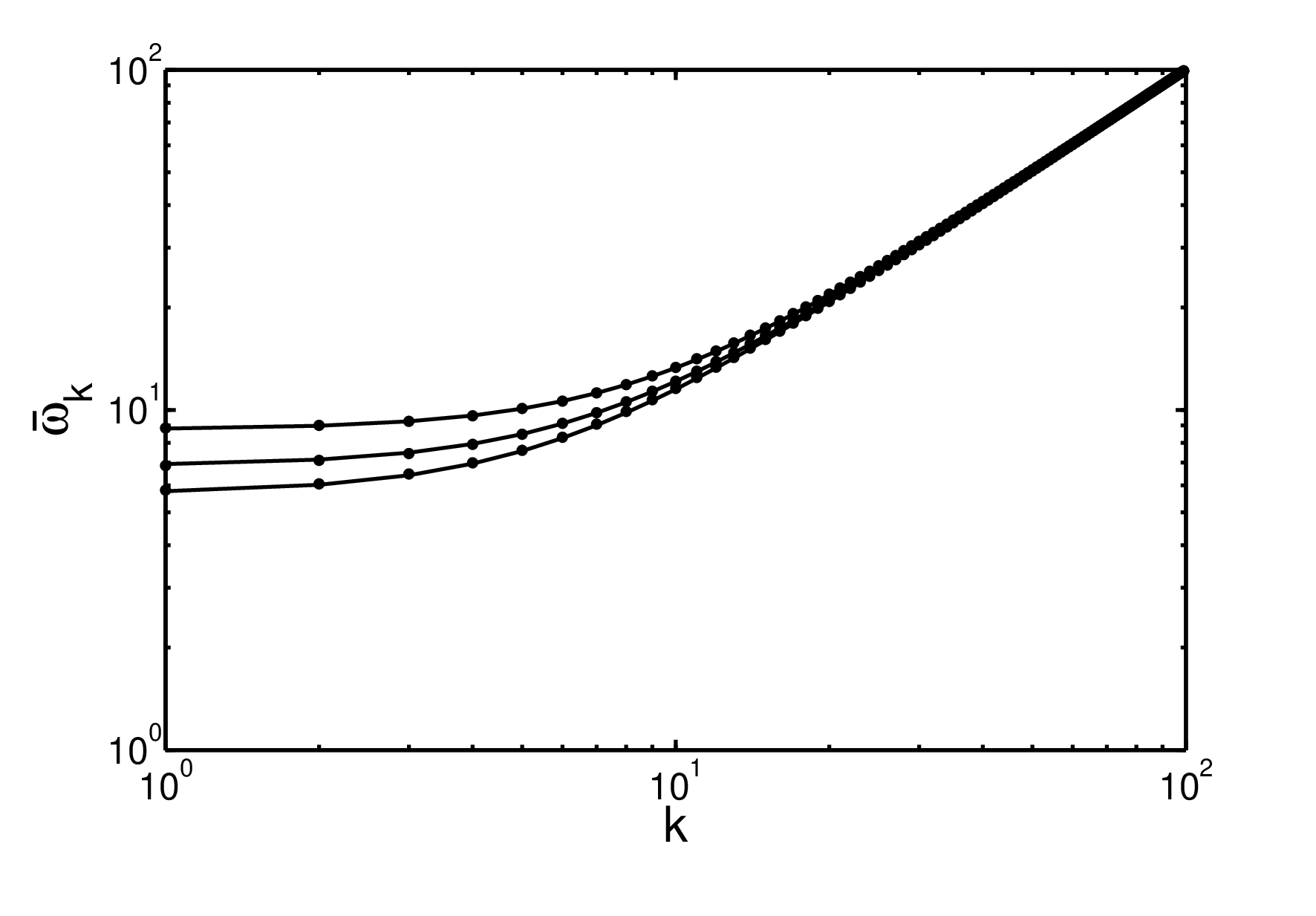
In addition to numerically computing $\tilde{\omega}_{k}$, we find that, in the case of strong nonlinearities, the frequencies always satisfy a shifted Klein-Gordon dispersion relation of the form

$$\tilde{\omega}_{k}^{2}\approx 1+2.59\lambda\langle S\rangle+k^{2}.$$

(40)

Again $S$ is the mean squared averaged field computed over the same time interval $(T_{1},T_{2})$ as $\tilde{\omega}_{k}$. For example, figure (11) shows the dispersion relation for several different initial conditions. Moreover, as a result of the LTE, both the value of $S$ and therefore $\tilde{\omega}_{k}$ drift over long times. Figure (3) verifies the relation (40) on two separate time intervals, with $\langle S\rangle=67.4$ on $(153,230)$ and $\langle S\rangle=60.24$ on $(767,843)$. Figure (4) also shows a plot of $S(t)$ highlighting the two averaging intervals. The deviation in $\langle S\rangle$ between the two intervals corresponds to a drift of roughly $5\%$ in the smallest frequency $\tilde{\omega}_{0}$.

Since the spatiotemporal transform verifies that the waves $c_{k}$ form narrow band oscillators centered at frequency $\tilde{\omega}_{k}$, we may introduce the effective energy [13] in Fourier mode $k$ in analogy with a linear oscillator

	$\displaystyle\langle E_{k}\rangle$	$\displaystyle=$	$\displaystyle\frac{1}{2}(\langle|p_{k}|^{2}\rangle+\tilde{\omega}_{k}^{2}\langle|u_{k}|^{2}\rangle)$		(41)
		$\displaystyle=$	$\displaystyle\langle|p_{k}|^{2}\rangle.$		(42)

Here the definition of the renormalized frequency over a given interval implies the waves on average satisfy the virial theorem, equally splitting the kinetic and potential energy. The quantity $\langle|p_{k}|^{2}\rangle$ therefore is a measure of the approximate energy in mode $k$, independent of renormalized frequency. Although the energy $E_{k}$ describes the modal distribution of energy, one should note that $\sum_{k}\langle E_{k}\rangle$ is not a conserved quantity and that the values of $\langle E_{k}\rangle$ exist only in an LTE state, and weakly depend on the interval $(T_{1},T_{2})$. The energy $E_{k}$ can also be related to the renormalized wave amplitudes via

$\displaystyle E_{k}=\frac{\tilde{\omega}_{k}}{2}\Big(\langle|c_{k}|^{2}\rangle+\langle|c_{-k}|^{2}\rangle\Big).$

(43)

Consequently, in the special case when $u_{k}=u_{-k}$, such as the initial data (39), then $E_{k}=\tilde{\omega}_{k}\langle|c_{k}|^{2}\rangle$ can also be used as a measure of energy in mode $k$.

In general, over the thermalization stage $(0,T_{1})$, solutions initialized to lower Fourier modes leak out into the higher modes. When viewed on a log scale, the energy spectrum evolves into a flat distribution in the low Fourier modes accompanied by a linear exponential decay in the high modes. For example, figure (5) shows the energy spectrum $\langle E_{k}\rangle$ averaged over the long time interval $(152,843)$. As solutions propagate through time, the spectrum retains a straight exponential decay, however the slope of decay may drift mildly (e.g., $10\%$) over time. We also calculate the sum $\sum_{k}\langle E_{k}\rangle\sim 6.8\times 10^{5}$ which differs from the exact energy $H\sim 6.7\times 10^{5}$ by $\approx 2.1\%$. Qualitatively, the spectrum appears very similar to the one predicted by the Planck blackbody distribution: $|c_{k}|^{2}\propto(e^{\beta\tilde{\omega}_{k}}-1)^{-1}$. The presence of a Planck-like spectrum arising from a classical system, such as a system of weakly coupled oscillators, is also discussed by Carati and Galgani [23]. For our data, the fit is only heuristic in that we can not simultaneous match the flat, long wave spectrum as well as the short wave exponential decay with a fixed temperature.

In addition to studying initial conditions (39) for $N=2048$ modes, we also performed several convergence tests with varying grid sizes $N=512,1024$, and $4096$ and different time steps $\Delta t$. We also found that numeric solutions do not depend on grid spacing provided the power spectrum remains exponentially suppressed over the integration times. For instance, $N=4096$ with initial (39) yields identical solutions to $N=2048$. Meanwhile, $N=512$ develops an energy cascade into the ultraviolet spectrum, accompanied by the onset of equipartition of energy. Hence, for the initial conditions (39), taking $N=2048$ yields a consistent solution to the PDE over the integration times $0<T<843$, while inconsistencies develop for smaller $N<1024$.

In addition to the power spectrum and renormalized dispersion relation, we also study the kinetic behavior of the LTE as well as fluctuations about equilibrium values. Since the frequency shift tracks the spatial average $S$, we plot $S$ as a function of time to gain an understanding of the dispersion relation evolution. Figure (4) shows the value $S$ over our integration time, along with a local time average value of $S$. We take the local time average $S$ over intervals long enough for the waves $c_{k}$ to exhibit numerous oscillations. Although the waves $c_{k}$ appear well defined for any fixed time interval $(T_{1},T_{2})$, there appears no well defined equilibrium, or more precisely if even the limit $\lim_{T\rightarrow\infty}\frac{1}{T}\int_{0}^{T}S\,\mathrm{d}t$ exists. As shown in figure (4), $S$ generally appears to decay, however drifts in time.

To further characterize the nature of the LTE, we examine fluctuations by plotting probability distributions of the squared field strength $S$ and energy spectrum for different time intervals. We find that for a sufficiently long time interval, $S$ acquires a Gaussian probability distribution with varying mean and width. Figure (6) shows the probability distribution $S$, as well as a Gaussian fit, over the interval $(153,230)$. Although not shown, the interval $(767,843)$ also exhibits a Gaussian probability distribution with a different mean. Only at very short time intervals, does $S$ not widen out to a Gaussian.

We also study the probability distributions (PDF) for wave amplitudes or particle numbers $|c_{k}|^{2}$. The distribution of these variables are related to the energy spectrum since one can identify $\tilde{\omega}_{k}|c_{k}|^{2}$ as the energy in mode $k$. Using the initial conditions (39) we plot the distribution of $|c_{k}|^{2}$ over the interval $(767,843)$ for different wave numbers. We find that low wave numbers, $k<200$, which achieve equipartition of energy, exhibit a classical Boltzmann distribution. For example figure (7) illustrates the distribution for mode $k=2$ along with an exponential fit of the form $e^{-\beta|c_{k}|^{2}}$. Meanwhile, the exponential distributions found in wave modes near the natural spectral cutoff, $k\approx 200$, start to shift their peaks away from $|c_{k}|^{2}=0$, as seen in figure (8). Lastly, there does not appear to be a consistent distribution of energy at large wavenumbers $k>200$. Specifically, adjacent modes $k$ and $k+1$ may exhibit very different distributions. Despite the lack of a unifying distribution, many large wave modes do exhibit a multipeaked distribution. Figures (9) and (10) show the amplitude distribution for $k=510$ and $k=520$, respectively.

References

- [1] G. B. Whitham, Linear and Nonlinear Waves, (John Wiley & Sons, New York, 1974).
- [2] S. Weinberg, The Quantum Theory of Fields, Vol. 1, (Cambridge University Press, Cambridge, 1995).
- [3] D. Boyanovsky, C. Destri, and H. J. de Vega, Phys. Rev. D 69, 045003 (2004).
- [4] S. Juchem, W. Cassing, and C. Greiner, Phys. Rev. D 69, 025006 (2004).
- [5] E. A. Calzetta, and B. L. Hu, [hep-ph/0205271] (2002).
- [6] G. Aarts, G. F. Bonini, and C. Wetterich, Nucl. Phys. B 587 (2000) 403-418.
- [7] G. Aarts, G. F. Bonini, and C. Wetterich, Phys. Rev. D 63, 025012 (2000).
- [8] M. Sall, J. Smit, and J. Vink, Nuclear Physics B, 625, (2002) 495-511.
- [9] J. A. Krumhansl, and J. R. Schrieffer, Phys. Rev. B 11, 3535 (1975).
- [10] D. J. Scalapino, M. Sears, and R. A. Farrell, Phys. Rev. B 6, 3409 (1972).
- [11] Here an LTE refers to a wave solution which exhibits characteristics of thermal equilibrium. For example, the distribution of Fourier mode wave energy for an LTE has a characteristic shape somewhat analogous to a Planck spectrum [3]. The term , however, refers to the fact that such distributions are defined only locally in time, and may drift slowly over longer time scales.
- [12] B. Gershgorin, Y. V. Lvov, and D. Cai, Phys. Rev. Lett. 95, 264302 (2005).
- [13] B. Gershgorin, Y. V. Lvov, and D. Cai, Phys. Rev. E 75, 046603 (2007).
- [14] W. Lee, G. Kovac̆ic̆, and D. Cai, Phys. Rev. Lett. 103, 024502 (2009).
- [15] M. Gleiser, Phys. Rev. D 49, 2978 (1994).
- [16] V. E. Zakharov, V. S. L’vov, and G. Falkovich, Kolmogorov Spectra of Turbulence I, (Springer, Berlin, 1992).
- [17] C. Guha-Roy, B. Bagchi, and D. K. Sinha, Int. J. Theor. Phys. 26, No. 4, (1987).
- [18] W. Press, B. Flannery, S. Teukolsky, and W. Vetterling, Numerical Recipes in C: The Art of Scientific Computing, (Cambridge University Press, Cambridge, 1988).
- [19] G. P. Berman, and F. M. Izrailev, The Fermi-Pasta-Ulam problem: 50 years of progress, Chaos 15, 015104 (2005).
- [20] The Fermi-Pasta-Ulam problem: A status report, Lect. Notes Phys., Vol. 728, edited by G. Gallavotti (Springer, Berlin, 2008).
- [21] G. Benettin, R. Livi, and A. Ponno, J. Stat. Phys. 135, 873-893 (2009).
- [22] The somewhat odd numerical values in the initial conditions found in Eq. (39), or even Table (1), arise as a consequence of normalization factors in the numerical fast Fourier transform. For instance, we used simple initial values in the numerical codes, however, converting these initial values with the definition (II.1), introduce extra numerical factors such as , resulting in more obscure values (i.e., ).
- [23] A. Carati and L. Galgani, Physica A 280 (2000).
- [24] E. Fermi, J. Pasta, and S. Ulam, Los Alamos Scientific Laboratory Report No. LA-1940 [reprinted in Fermi E. Collected papers (University of Chicago Press, Chicago, 1965), Vol II, p. 978].
- [25] R. Livi, M. Pettini, S. Ruflo, and A. Vulpiani, J. Phys. A: Math. Gen. 20 (1987) 577-586.
- [26] Patrasciou A., Phys. Lett. 104A 87 (1984).
- [27] J. De Luca, and A. Lichtenberg, Phys. Rev. E 66, 026206 (2002).
- [28] M. Abramowitz and I. A. Stegun, Handbook of Mathematical Functions, (Dover Publications, Inc., New York, 1972).