Rank $k$ Cholesky Up/Down-dating on the GPU: gpucholmodV0.2

Given a symmetric positive definite matrix $A\in\mathbb{R}^{n\times n}$, for reasons of computational efficiency and stability, it is often indispensable that we are able to maintain the upper triangular Cholesky factor $L$ such that $A=L^{\top}L$ — see [1] for a discussion. Frequently, $A$ will changes by low rank modification during the course of an algorithm, hence it is imperative that we can accordingly modify the associated Cholesky factor $L$ in an efficient and stable manner, in order to maintain an optimal asymptotic time complexity. We focus on the following problem: given $A$, $L$, and a matrix $V\in\mathbb{R}^{n\times k}$, form the modified factor $\tilde{L}$ such that $\tilde{L}^{\top}\tilde{L}=A\pm VV^{\top}=\tilde{A}$. In particular we do so with $\mathcal{O}(kn^{2})$ operations, rather than by naïvely computing the modified matrix $\tilde{A}$ and from there rebuilding the full Cholesky factor. This is referred to as the rank $k$ Cholesky up (down) date when dealing with addition (subtraction) of $VV^{\top}$. Existing CPU implementations such as dchud of LINPACK [2] typically treat the case $k=1$. We allow $k>1$ since this leads to more efficient memory access, although speedups are also obtainable with our algorithm for $k=1$ (naturally this demands a larger problem size $n$, however).

The serial algorithm which we will adapt to the GPU is the so called hyperbolic approach which we state as Algorithm 1 for the case $k=1$.

Let us take stock of the memory accesses in the inner loop of the two possible orderings in Algorithm 1:

• •

  In CholeskyModifyA we read $c_{j},s_{j}$ and $L_{j,i}$, and write $L_{j,i}$. The $V_{i}$ must only be read and written before and after the inner loop.

• •

  In CholeskyModifyB we read and write $L_{i,j}$ and $V_{j}$. In this case, it is $c_{i}$ and $s_{i}$ which need only be read and written before and after the inner loop.

Hence we see that if reading and writing were equally costly, then the ordering of CholeskyModifyA would be slightly better — not only that, but CholeskyModifyA also offers a rather natural mapping to the GPU shared and register memory of current hardware, as we shall see in the following subsection, so this is the approach we will employ. We make no claim as to the optimality of this approach — if the reader is aware of a superior approach, we would be interested to hear about it.

A GPU kernel function which computes the inner loop of CholeskyModifyA would need to be launched $n$ times. To avoid the overhead inherent in these repeated kernel launches we proceed by computing larger submatrices of $L$, sequentially and either on the CPU or the GPU. The panelling strategy, which is illustrated in Figure 1, will be described in this section.

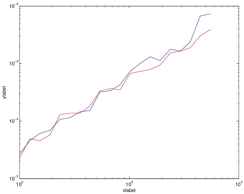
To give the reader an idea of roughly what our GPU algorithm might buy them in terms of speedups, we present some basic timings in figures 2 and 3. The experimental procedure involves forming the matrices $B\in\mathbb{R}^{n\times n}$ and $V\in\mathbb{R}^{n\times k}$ with elements drawn i.i.d. from the uniform distribution on $[0,1]$. In the update test we let $A=B^{\top}B+I$, where $I$ is the identity matrix, and compute the Cholesky factor $L$ using the LAPACK algorithm [3] and update it by $V$. For the downdating test we let $A=B^{\top}B+I+VV^{\top}$ and downdate by $V$. Errors are calculated as $\text{max}_{i,j}\left|\tilde{A}_{i,j}-C_{i,j}\right|$ where $C=\tilde{L}^{\top}\tilde{L}$ is computed with the BLAS and $\tilde{L}$ is computed from $L$ by up/down-dating $L$. The experiment is repeated for $k=16$ and $k=1$ in figures 2 and 3, respectively. For the CPU up/down-dating we used the LAPACK suite.

The test system was a desktop machine running 64 bit Ubuntu linux with a 2.8GHz Intel i7 CPU and an Nvidia Tesla C2050 GPU with 14 streaming multiprocessors and a total of 448 cores and CUDA version 3.10. Note that the number of cores on the GPU is relatively unimportant however, due to the bandwidth bound nature of the problem.

The experiments show that for $k=16$, the GPU overtakes the CPU at around $n=2000$, while for $k=1$ we require at least $n=4000$ in order to break even with the CPU. The errors are always very similar. Note that much larger problems can be handled since we only store $\mathcal{O}(n)$ sized panels of $L$ in device memory, unfortunately however our test system had rather limited host memory.

References

- [1] Seeger, M.: Low rank updates for the cholesky decomposition. Technical report, University of California, Berkeley (2004)
- [2] Dongarra, J.J., Moler, C.B., Bunch, J.R., Stewart, G.W.: LINPACK User’s Guide. SIAM (1979)
- [3] Anderson, E., Bai, Z., Bischof, C., Blackford, S., Demmel, J., Dongarra, J., Croz, J.D., Greenbaum, A., Hammarling, S., McKenney, A., Sorensen, D.: LAPACK Users’ Guide. Third edn. Society for Industrial and Applied Mathematics, Philadelphia, PA (1999)