Cluster Abundance in Gravity Models
Abstract
As one of the most powerful probes of cosmological structure formation, the abundance of massive galaxy clusters is a sensitive probe of modifications to gravity on cosmological scales. In this paper, we present results from -body simulations of a general class of models, which self-consistently solve the non-linear field equation for the enhanced forces. Within this class we vary the amplitude of the field, which controls the range of the enhanced gravitational forces, both at the present epoch and as a function of redshift. Most models in the literature can be mapped onto the parameter space of this class. Focusing on the abundance of massive dark matter halos, we compare the simulation results to a simple spherical collapse model. Current constraints lie in the large-field regime, where the chameleon mechanism is not important. In this regime, the spherical collapse model works equally well for a wide range of models and can serve as a model-independent tool for placing constraints on gravity from cluster abundance. Using these results, we show how constraints from the observed local abundance of X-ray clusters on a specific model can be mapped onto other members of this general class of models.
I Introduction
The abundance of massive galaxy clusters provides a unique test of gravity on cosmological scales [1, 2, 3]. Once constrained to expansion history data, modified gravity explanations of the cosmic acceleration generically predict very different effects on the growth of cosmological structure than spatially smooth dark energy like the cosmological constant. Moreover as highly non-linear objects, clusters provide a testing ground for the non-linear interactions of viable theories where gravity becomes indistinguishable from General Relativity locally.
In the so-called class of models (see [4, 5] and references therein) the modification to gravity arises from replacing the Einstein-Hilbert action by a function of the Ricci or curvature scalar [6, 7, 8]. These models possess an extra scalar degree of freedom which mediates a 4/3 enhancement of gravitational forces on scales below the Compton wavelength or range associated with its mass.
This enhancement changes the abundance of rare dark matter halos associated with clusters of galaxies. Measurements of the cluster abundance provide the current best cosmological constraints on models [1, 3]. On the other hand, in order to hide these enhancements from local tests of gravity, viable models employ the chameleon mechanism which allows the Compton wavelength to shrink in regions with deep gravitational potential wells [9, 10]. Cosmological simulations including the chameleon effect are required to explore the impact of these modified forces on the cluster abundance. These have so far been performed for only a specific form of [11, 12, 13].
In fact, the relationship between the Compton wavelength, chameleon threshold and their respective evolution with redshift depends on the functional form of . In this paper, we explore the dependence of the cluster abundance on the functional form of in order to place more robust constraints on the whole class of models.
In §II, we review the phenomenology of models, simulation technique and spherical collapse modeling as well as show that a general class of broken power law models introduced in Ref. [14] covers most cases of cosmological interest. In §III we study the enhancement of the cluster abundance in these models and obtain constraints from the local X-ray sample. We discuss these results in §IV.
II Methodology
We begin in §II.1 with a review of models. In §II.2 we discuss the numerical -body simulations from which we extract the cluster abundance enhancements. In §II.2, we discuss the semi-analytic modeling of these results with spherical collapse collapse calculations.
II.1 Models
In the model, the Einstein-Hilbert action is augmented with a general function of the scalar curvature ,
| (1) |
Here and throughout . Gravitational force enhancements are associated with an additional scalar degree of freedom, the chameleon field , and have a range given by the comoving Compton wavelength . This additional attractive force leads to the enhancement in the abundance of rare massive dark matter halos described below. The second important property of such models is the non-linear chameleon effect which shuts down the enhanced forces in regions with deep gravitational potential wells compared with the field at the background curvature , .
Given that different models for produce different scalings of the Compton wavelength and chameleon threshold with curvature and hence implicitly with redshift and the degree of non-linearity, we wish to explore the dependence of the halo abundance with variations in the form of .

We therefore choose a class of models where the scaling index with curvature can vary as a broken power law [14] such that
| (2) |
with two free parameters, , for each value of the scaling index . Note that as , , and hence these models do not contain a cosmological constant. Nonetheless as , the function can be approximated as
| (3) |
with replacing as the second parameter of the model. Here we define , so that , where overbars denote the quantities of the background spacetime. Note that if the curvature scales set by and differ widely and hence the approximation is valid today and for all times in the past.
The background expansion history mimics CDM with as a true cosmological constant to order . Therefore in the limit , the model and CDM are essentially indistinguishable with geometric tests. On the other hand, the field amplitude parameter () controls the range of the force modification and the chameleon mechanism. With the functional form of Eq. (3), the comoving Compton wavelength becomes
| (4) |
with a value at the background curvature today of
| (5) |
assuming a flat universe. As the scaling index increases, the Compton wavelength today increases given the same background field amplitude today . Conversely as increases, force modifications at high redshift versus today decrease and the chameleon mechanism extends to shallower potential wells. Thus the net effect is a fairly weak dependence of on at . In Fig. 1, we show the evolution of the background field and Compton wavelength for the , cosmology that we simulate below.
This set of broken power law models covers the cosmological phenomenology of most viable models. For example the models of Ref. [15] compose a subset of this class. It also has sufficient flexibility to bracket the behavior of models where the combination of a specific expansion history [16, 17] and the Compton wavelength today fixes the form of [18]. For the CDM expansion history and a dimensionless Compton wavelength parameter
| (6) |
where , the redshift evolution goes from at low curvature and redshift to at high curvature and redshift (see Fig. 1). For a fixed the amount of linear growth at in the model is smaller than in the model and this must be borne in mind when comparing constraints between the two models (cf. [1, 3, 19]).
Likewise these models have stronger chameleon effects at than the broken power law model. A similar caveat applies to models with exponential rather than power law suppression of the field with curvature (e.g. [20]).
II.2 Simulations
We conduct -body simulations of these broken power law models with a particle-mesh relaxation code [11, 12]. Briefly, at each time step we first solve the non-linear field equation for the field fluctuation,
| (7) |
using a multigrid relaxation scheme. Here coordinates are comoving, , , . The field fluctuation then acts as an additional source to the gravitational potential,
| (8) |
This linear equation for is solved via a fast Fourier transform. Once is known on the mesh, particles are moved in the usual way.
Since the field equation implies that spatial variations in will be of order the gravitational potential, there are two regimes of interest. In the large-field regime, the background value is large compared with the gravitational potentials of structure, and the field equation (7) can be linearized via
| (9) |
where is evaluated at the background curvature . In this case the joint solution of the Poisson and field equations in Fourier space is
| (10) |
Hence the background Compton wavelength sets the global range of the enhanced gravitational force. We call this the no chameleon case and for comparison conduct separate simulations employing Eq. (10).
In the small-field regime, is comparable to or smaller than typical gravitational potentials of structure, so that the curvature changes non-linearly with the field. In other words the Compton wavelength depends on the local curvature or field . Field fluctuations saturate in deep gravitational potential wells (), leading to an equilibrium solution and a suppression of non-Newtonian forces.
We use simulations of three different box sizes (), and 6 simulations for each box size and model. The runs and models as well as mass resolution for each box are summarized in Table 1. To reduce the effect of sample variance, we compare each simulation run to a CDM simulation with the same initial conditions, i.e. the same initial density field drawn from an initial power spectrum with at Mpc-1 and .
We measure the mass function from the simulations using the methodology described in [13] and refer the reader to details therein. Briefly, we identify halos using a spherical overdensity criterion of with respect to the mean density and quantify the mass function enhancements of the models over CDM with the same initial conditions. To reduce the effect of shot noise we bin results into coarse mass intervals corresponding to approximately an e-fold (). Furthermore, due to resolution effects, we only utilize halos that contain at least 800 particles corresponding to the minimum mass given in Tab. 1.
We estimate sampling errors via bootstrap resampling. Note that due to our limited number of realizations, these errors might be underestimated at high masses where halos are rare and fluctuations are significant.
| ( Mpc) | ||||
| # full | (=1, 2) | 6 | 6 | 6 |
| runs | (=2) | 6 | 6 | 6 |
| (=1) | 6 | 6 | 6 | |
| # no | (=1/2, 1, 2, 4, 8) | 6 | 6 | 6 |
| cham. runs | (=2) | 6 | 6 | 6 |
| (=1) | 6 | 6 | 6 | |
| CDM | 0 | 6 | 6 | 6 |
| () | 204 | 53.7 | 6.61 | |
II.3 Spherical Collapse Predictions
Since the large field regime is where the current local cluster abundance measurements constrain models [1, 3], characterizing this regime in a way that does not require simulations of each model is important. We briefly review a method utilizing spherical collapse introduced in Ref. [13]
The Sheth-Tormen description for the comoving number density of halos per logarithmic interval in the virial mass is given by
| (11) |
where the peak threshold and
| (12) |
Here is the variance of the linear density field convolved with a top hat of radius that encloses at the background density
| (13) |
where is the linear power spectrum and is the Fourier transform of the top hat window. The normalization constant is chosen such that . The parameter values of , , and for the spherical collapse threshold have previously been shown to match simulations of CDM at the level. The virial mass is defined as the mass enclosed at the virial radius , at which the average density is times the mean density. The virial mass can then be transformed to alternate overdensity criteria assuming a Navarro-Frenk-White density profile [21].
Spherical collapse can also provide a model for the mass function enhancement measured in the -body simulations [13]. The mass function calculation again uses the Sheth-Tormen form of Eq. (11) but with the linear power spectrum for the model in Eq. (13), and two limiting cases for the spherical collapse parameters. In one case, we simply assume that the spherical perturbation considered is always larger than the Compton wavelength of the field, so that gravity is GR throughout, and the spherical collapse parameters are unchanged. In the second case, we assume that the perturbation is always smaller than the local Compton wavelength in spite of the redshift evolution of the background Compton wavelength and chameleon mechanism (see Fig. 1). Hence forces are simply universally enhanced by 4/3. In both cases, we use the modified linear force calculation for the linear power spectrum and via Eq. (11). Hence, unmodified spherical collapse parameters does not equate to unmodified spherical collapse predictions.
The values of the resulting linear collapse threshold and virial overdensity are summarized in Table 2. We use the GR values to calculate the mass function Eq. (11) in terms of virial mass () for CDM, and correspondingly for with either set of collapse parameters. We then rescale both mass functions to our adopted mass definition and convolve them with the mass binning used in the simulations before taking the ratio.
| GR | mod. forces | GR | mod. forces | |
| 1.673 | 1.692 | 1.679 | 1.697 | |
| 391 | 309 | 279 | 222 | |

III Cluster Abundance
With the simulations described in Tab. 1, we can now test the model dependence of the cluster abundance enhancement as well as the accuracy of the model-independent spherical collapse technique described in the previous section. In §III.1 we discuss the large field regime relevant for current constraints from clusters. In §III.2 we evaluate the impact of the non-linear chameleon mechanism in the small field regime. Finally we show how constraints on one model can be transformed to another using simulation calibrated spherical collapse methods in §III.3.
III.1 Large Field Regime
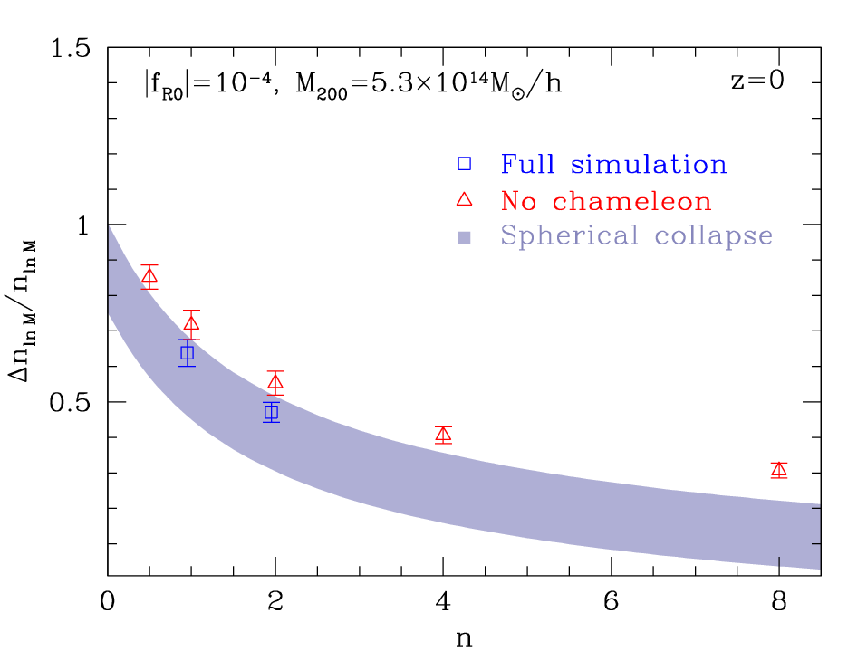
In Fig. 2, we show the mass function enhancements for a large field case for . Note that we plot the data points at the center of each mass bin, while the average mass of halos within the bin is generally smaller than that due to the steepness of the mass function. The spherical collapse predictions are convolved with the mass bin and hence take into account this effect. The uppermost mass bin extends to infinite mass so as to include all remaining halos but is still plotted at above the previous bin.
As the mass increases and halos become rarer in the CDM simulations, the fractional impact of the force enhancement on cluster abundance increases. Relative to this overall enhancement the impact of changing the scaling parameter is less significant. This weak dependence is in spite of the rapid change in the background field shown in Fig. 1.
We can understand this relative insensitivity by comparing the full simulation results to the no-chameleon simulations where the Compton wavelength is fixed to its background value through Eq. (10). Mass function enhancements in the chameleon and no-chameleon simulations are nearly the same up until the very highest masses. For the large field value today , cluster potential wells are not sufficiently deep to manifest the chameleon mechanism today. The small effect at the very highest masses in fact comes from the chameleon mechanism becoming effective at high redshift as we shall see. One can in turn understand the relative insensitivity to in the no-chameleon simulations by examining the background Compton wavelength evolution in Fig. 1. Note that for , the Compton wavelength varies little for redshifts .

The spherical collapse predictions outlined in the previous section are also shown in Fig. 2. The upper boundary of the shaded region represents enhancements predicted by the unmodified spherical collapse parameters and whereas the lower boundary takes the modified parameters and (Table 2).
The spherical collapse predictions model the results equally well for the and models. In the high mass cluster regime, the unmodified parameters match the simulations better. In the low mass end the modified parameters agree better. The modified parameters also provide conservative estimates of the enhancements across the full mass range [13].
We further test the large-field no-chameleon simulations against spherical collapse predictions for even steeper models in Fig. 3. These predictions, based mainly on the instantaneous linear growth function, remain accurate despite the extremely strong scaling of the force modification with redshift in these models. Furthermore, Fig. 1 implies that the no-chameleon results should be a reasonable approximation to the full simulations for . Thus, in the large field regime, one way to map cluster constraints obtained at a given mass on one model to another is to match the linear variance . A better approximation can be obtained by setting the mass function equal as we shall see in §III.3.
In Fig. 4, we show the mass function enhancements at an intermediate redshift for the large field model. Note that the abundance of halos of mass at is equal to that of halos of mass at this redshift in a CDM model, due to the evolution of the mass function, and we have adjusted our binning to take this into account. Thus for a fixed mass, the enhancement in the cluster abundance remains significant. Interestingly, the range in spherical collapse predictions continues to model these trends once the collapse parameters are adjusted to the matching redshift (see Tab. 2).
The results at show a slight increase in the importance of the chameleon suppression when compared to or at the same redshift. This is consistent with the suppression of the field amplitude shown in Fig. 1. For , the effect is only a small fractional contribution and spherical collapse predictions still work well but suggest that the no-chameleon approximation may have a smaller range of validity in at high redshift. More generally modified gravity models which possess this type of non-linearity that suppresses deviations in high density regions typically do not predict larger enhancements of the cluster abundance at high versus low redshift at a fixed degree of rarity or peak height [22].

III.2 Small Field Regime
As cluster abundance and other cosmological tests improve, the large-field models will be excluded (if no order unity excesses over CDM expectations are detected). In the small field regime of , the chameleon mechanism is effective even today.
In Fig. 5, we show small field results for and and, for , . The first thing to note is that in the no chameleon simulations the impact of changing the field value from to is less than a factor of 2 in the abundance at the highest mass bin. We shall see in the next section, that this logarithmic sensitivity translates into a strong model dependence of observational constraints on the field amplitude and Compton wavelength.
Small field results show a large impact from the chameleon suppression as can be seen by comparing the full simulations to the no-chameleon simulations. A halo is chameleon-screened whenever its gravitational potential is larger than the field amplitude in the background . This can be used to derive a threshold mass for chameleon screening at for a given value of (see [23]). We then expect the mass scale of the chameleon suppression in the mass function to scale similarly as the threshold for chameleon screening. In particular, should depend mainly on and only weakly on the scaling index . Specifically, neglecting the small mass-dependence of the halo concentration, we would expect the onset of the chameleon suppression to scale as .
We see from Fig. 5 that the results are consistent with this scaling: roughly, the chameleon for is important for while for , the suppression appears at . The , case falls consistently right in between the two despite being a different model.
Spherical collapse predictions roughly model the reduced enhancement in the cluster regime of . They correctly predict an absence of a significant enhancement for . However, unmodified collapse parameter predictions can fractionally overestimate the enhancement unlike in the large field regime, while modified collapse parameter predictions predict a reduction in the cluster abundance () not seen in the simulations. Moreover both cases do not predict the correct behavior at lower masses where the full simulations possess a higher abundance of halos than both the no-chameleon simulations and the collapse predictions. Hence in the small field regime they should not be used for constraints from galaxy groups or smaller mass objects or if precision predictions are required at cluster masses. We defer such modeling to a future work.

III.3 Current Constraints
Given that spherical collapse predictions work equally well for all of our broken power law models with in the cluster regime and capture the scalings seen in the full simulations, we can extend the constraints on the model with [1] that were obtained using the observed abundance of local X-ray clusters selected in the ROSAT All-Sky Survey and followed up with Chandra observations [24].
The constraints were obtained by using the spherical collapse model (see section II.3) to predict the mass function enhancement at a pivot mass of , for an overdensity of 500 with respect to critical density. Fig. 3 shows that the spherical collapse model is equally valid for other values of as long as the chameleon effect is negligible, and it is straightforward to translate the constraints to other values of by matching the abundance at .
The results are shown as function of in Fig. 6 for a range of conservative to aggressive interpretations of the data and modeling (see [1] for further discussion). In the top panel we show the 95% statistical limits on the field amplitude today and in the bottom panel the Compton wavelength in the background today . The medium shaded region shows the result for the default constraint, at , using the modified spherical collapse parameters (lower edge of shaded band in Fig. 3). The dark region shows the most conservative constraints (), using the modified collapse parameters and in addition assuming X-ray masses are underestimated by 9%. Finally, the light region shows more aggressive constraints (), using the unmodified collapse parameters (upper edge of shaded band in Fig. 3). Note that even this case is still somewhat conservative, since for clusters at fixed mass, dynamical mass estimates such as X-ray masses will be enhanced by in the large-field limit of gravity [23], due to the increased depth of the potential well. This increases the abundance at fixed in considerably.
While the change in the fractional enhancement of the mass function from CDM with is relatively small, the impact on the model parameters can be large. Specifically between the and models the field amplitude limits change by over an order of magnitude and Compton wavelength constraints by a factor of several.
Nonetheless the cluster abundance measurements can already rule out a substantial portion of the cosmologically interesting regime for all cases, limiting the allowed range of enhanced forces to Mpc. Future large cluster samples have the potential to push the limits down by an order of magnitude before chameleon effects cause a suppression of the enhancement.
IV Discussion
We have conducted -body simulations to test the enhancement of the cluster abundance in a variety of models. These models differ in the redshift evolution of both the linear force enhancement and the non-linear chameleon mechanism which suppresses such enhancements in the deep gravitational potential wells of clusters of galaxies. These results test the robustness of model independent techniques such as spherical collapse for predicting the enhancement and constraining modified gravity with cosmological data.
We find that for cluster mass halos, the spherical collapse predictions work equally well for different models at least as long as the redshift evolution of the field is not so steep as to invalidate the division between large field and small field regime imposed at for the background field amplitude at . In the large field regime the background field amplitude is larger than the depth of the gravitational potential wells of clusters and hence the chameleon effect is inoperative. For a scaling index , a large field model retains this property for when clusters form. In this regime, the fractional enhancement of the cluster abundance relative to CDM is a relatively weak function of that is determined by the evolution of the Compton wavelength or range of the force in the background. In the opposite small field regime, the enhancements become suppressed above a limiting mass that depends mainly on the field amplitude .
We use these results to extend the implications of the local cluster abundance to the whole class of broken power law models. Most models in the literature can be mapped onto the parameter space of this class. Constraints on the field amplitude and Compton wavelength today are strongly model dependent due to the logarithmic dependence of the cluster abundance on their values in any given model.
Results based on different model assumptions can be mapped onto each other by matching instead the linear theory rms fluctuation at the radius implied by the observed mass scale or even more directly by matching spherical collapse mass function predictions as we have shown for the local -ray cluster abundance.
Acknowledgments: SF and WH were supported by the Kavli Institute for Cosmological Physics (KICP) at the University of Chicago through grants NSF PHY-0114422 and NSF PHY-0551142 and an endowment from the Kavli Foundation and its founder Fred Kavli. SF was additionally supported by Eugene and Niesje Parker and Robert G. Sachs fellowships. WH was additionally supported by U.S. Dept. of Energy contract DE-FG02-90ER-40560 and the David and Lucile Packard Foundation. FS was supported by the Gordon and Betty Moore Foundation at Caltech. Computational resources for the cosmological simulations were provided by the KICP-Fermilab computer cluster.
References
- [1] F. Schmidt, A. Vikhlinin and W. Hu, Phys. Rev. D80, 083505 (2009), [arXiv:0908.2457].
- [2] D. Rapetti, S. W. Allen, A. Mantz and H. Ebeling, Mon. Not. R. Astron. Soc. 406, 1796 (2010), [arXiv:0911.1787].
- [3] L. Lombriser, A. Slosar, U. Seljak and W. Hu, arXiv:1003.3009.
- [4] S. Nojiri and S. D. Odintsov, Int.J.Geom.Meth.Mod.Phys. 4, 06 (2006), [arXiv:hep-th/0601213].
- [5] T. P. Sotiriou and V. Faraoni, Rev. Mod. Phys. 82, 451 (2010), [arXiv:0805.1726].
- [6] S. Capozziello, Int.J.Mod.Phys. D11, 483 (2002), [arXiv:gr-qc/0201033].
- [7] S. Nojiri and S. D. Odintsov, Phys. Rev. D68, 123512 (2003), [arXiv:hep-th/0307288].
- [8] S. Capozziello, S. Carloni and A. Troisi, Recent Res. Dev. Astron. Astrophys. 1, 625 (2003), [arXiv:astro-ph/0303041].
- [9] D. F. Mota and J. D. Barrow, Phys. Lett. B581, 141 (2004), [arXiv:astro-ph/0306047].
- [10] J. Khoury and A. Weltman, Phys. Rev. D69, 044026 (2004), [arXiv:astro-ph/0309411].
- [11] H. Oyaizu, Phys. Rev. D78, 123523 (2008), [arXiv:0807.2449].
- [12] H. Oyaizu, M. Lima and W. Hu, Phys. Rev. D78, 123524 (2008), [arXiv:0807.2462].
- [13] F. Schmidt, M. V. Lima, H. Oyaizu and W. Hu, Phys. Rev. D79, 083518 (2009), [arXiv:0812.0545].
- [14] W. Hu and I. Sawicki, Phys. Rev. D76, 064004 (2007), [arXiv:0705.1158].
- [15] A. A. Starobinsky, JETP Lett. 86, 157 (2007), [arXiv:0706.2041].
- [16] T. Multamaki and I. Vilja, Phys.Rev. D73, 024018 (2006), [arXiv:astro-ph/0506692].
- [17] S. Capozziello, S. Nojiri, S. Odintsov and A. Troisi, Phys.Lett. B639, 135 (2006), [arXiv:astro-ph/0604431].
- [18] Y.-S. Song, W. Hu and I. Sawicki, Phys. Rev. D75, 044004 (2007), [arXiv:astro-ph/0610532].
- [19] S. A. Appleby and J. Weller, arXiv:1008.2693.
- [20] S. A. Appleby and R. A. Battye, Phys. Lett. B654, 7 (2007), [arXiv:0705.3199].
- [21] W. Hu and A. V. Kravtsov, Astrophys. J. 584, 702 (2003), [arXiv:astro-ph/0203169].
- [22] M. J. Mortonson, W. Hu and D. Huterer, arXiv:1011.0004.
- [23] F. Schmidt, Phys. Rev. D81, 103002 (2010), [arXiv:1003.0409].
- [24] A. Vikhlinin et al., Astrophys. J. 692, 1060 (2009), [arXiv:0812.2720].