Transverse-Spin and Transverse-Momentum Effects
in High-Energy Processes
Abstract
The state of the art concerning transverse-spin and transverse-momentum
phenomena in hard hadronic reactions is reviewed.
An account is given of single-spin and azimuthal asymmetries
in semiinclusive deep inelastic scattering, annihilation,
Drell-Yan production, and hadroproduction.
The ongoing experiments and the main theoretical frameworks
are described in the first part of the paper. The second part
is devoted to the experimental findings and their phenomenological
interpretations.
A brief discussion of the perspectives of future measurements is
finally presented.
1 Introduction
For quite a long time the common lore in the hadron physics community has been that transverse polarisation effects are negligibly small in hard processes. In the last two decades a growing theoretical and experimental evidence has shown that this is not the case and that transverse-spin phenomena are, on the contrary, rather relevant in various high-energy hadronic reactions.
The prehistory of the subject started in the mid-70s, when substantial single-spin asymmetries (SSA’s) were found in inclusive pion hadroproduction at the center-of-mass energies of the Argonne synchrotron (few GeV) [1, 2, 3]. At the same time, at Fermilab hyperons produced in unpolarised collisions at GeV and moderate transverse momenta (below 1.5 GeV) were found to possess a large transverse polarisation [4], a result subsequently confirmed at slightly higher and [5].
These findings stimulated both experimental and theoretical work. An experimental programme to investigate both longitudinal and transverse spin effects in high energy and scattering was proposed in 1978 at FNAL [6] and carried out more than 10 yeas later by the E704 Collaboration. Measuring inclusive pion production in collisions of transversely polarised proton and antiproton beams with an hydrogen target at the center-of-mass energy GeV and for up to 2 GeV, the E704 Collaboration found single-spin asymmetries as large as 40 % in the forward region [7, 8, 9, 10]. More recently, the experimental collaborations STAR, PHENIX and BRAHMS, working at RHIC, have confirmed the early Fermilab findings on single-spin asymmetries in hadroproduction, pushing the frontier of the c.m. energy to GeV and covering wider kinematical ranges in and in the Feynman variable [11, 12, 13, 14, 15].
On the theoretical side, soon after the first experimental findings of transverse spin effects, Kane, Pumplin and Repko proved in a famous paper [16] that in collinear perturbative QCD (applicable to high ) SSA’s are of the order of (where is the quark mass) and therefore vanish in the massless limit. Also, in other important theoretical works [17, 18, 19] it was shown that non-vanishing transverse single-spin asymmetries may arise in QCD only if one consider higher-twist contributions (naïvely expected to behave as a power of , where is a hadronic scale.
It took a while to realise that theory allows for transverse polarisation effects which are in some cases unsuppressed (for a review see f.i. Ref. [20]). In the early 90s various authors [21, 22, 23, 24] rediscovered the distribution of transversely polarised quarks in a transversely polarised nucleon first introduced by Ralston and Soper in 1979 [25]. This “transversity” distribution, usually denoted by or by , is a leading-twist quantity that contributes dominantly to the double transverse asymmetry in Drell-Yan (DY) production. Due to its chiral-odd nature is not measurable in inclusive Deep Inelastic Scattering (DIS), where transverse SSA’s are prohibited by time-reversal invariance at lowest order in [26]. This argument, however, does not hold in semi-inclusive DIS (SIDIS), where at least one hadron in the final state is detected on top of the scattered lepton. In SIDIS processes no first principles forbid SSA’s. Various theoretical proposals were soon put forward to measure [27, 28, 29, 30, 31, 32, 33]. In particular, Collins proposed a mechanism, based on a spin asymmetry in the fragmentation of transversely polarised quarks into an unpolarised hadron (the “Collins effect”), which involves a transverse-momentum dependent (TMD) fragmentation function, . This mechanism was originally proposed as a “quark polarimeter”, and could be conveniently exploited to measure the transversity function in SIDIS.
In a different approach, one year before the publication of the E704 results, Sivers had suggested that single-spin asymmetries could originate, at leading twist, from the intrinsic motion of quarks in the colliding hadrons [34, 35]. The idea, in particular, was that there exists an azimuthal asymmetry of unpolarised quarks in a transversely polarised hadron (the so-called “Sivers effect”), and a new -odd TMD distribution function, now commonly called Sivers function and usually denoted by , was proposed to describe the partons in a transversely polarised nucleon.
Originally this mechanism seemed to violate time-reversal () invariance [29] and it was demonstrated that had to be zero. Brodsky, Hwang and Schmidt [36, 37] proved however by an explicit calculation that final-state interactions in SIDIS, arising from gluon exchange between the struck quark and the nucleon remnant, or initial-state interactions in DY, produce a non-zero Sivers asymmetry. The situation was further clarified by Collins [38] who pointed out that, taking correctly into account the gauge links in the TMD distributions, time-reversal invariance does not imply a vanishing , but rather a sign difference between the Sivers distribution measured in SIDIS and the same distribution measured in DY.
The phenomenological analysis of the E704 results [39, 40], however, showed that both the Collins and the Sivers effects are at work to generate the observed asymmetries, but a satisfactory theoretical description of the data is still missing today.
New experimental opportunities came out in the 90’s, when it was realised that high energy SIDIS experiments were needed to investigate the helicity structure of the nucleons. In fact a major event had focused on the nucleon spin the attention of the high energy physics community. In 1988 the EMC Collaboration at CERN, scattering a high energy polarised muon beam on a transversely polarised proton target obtained a totally unexpected result, namely that the fraction of the nucleon spin carried by the quarks was small, even compatible with zero, within the accuracy of the measurement. From the inclusive cross-section difference for parallel and antiparallel spins one could extract a linear combination of the quark helicity distributions (or ), defined as the difference of the quark densities for quark spin parallel or antiparallel to the longitudinal nucleon spin. Using complementary information on the quark helicities derived from the weak decays of the hyperons it was possible to add up the quark helicities, thus obtaining , the overall quark contribution to the nucleon spin. The result, which came to be known as the “spin crisis” was at variance with the current paradigm, i.e. the quark model and the beautifully simple explanation of the baryon magnetic moments. More than one thousand theoretical papers were written on the subject, and many experiment (SMC at CERN, E142, E143, E154 and E155 at SLAC) were proposed and executed to confirm the effect, to extend the result to the neutron, and to improve the accuracy of the measurement. The confirmation of this finding led to a growing attention to the other contributions to the proton spin, namely the gluon polarisation and the orbital angular momentum of both quarks and gluons, as well as to a deeper look at the QCD description of the nucleon and to the relation between and . Thus, new generation experiments, well suited to investigate SIDIS with both longitudinally and transversely polarised targets, like COMPASS and HERMES, were proposed and started their operations about 10 years ago.
In 2004 HERMES [41] and COMPASS [42, 43] presented the first data collected with transversely polarised proton and deuteron targets, which showed clear evidence of transverse SSA’s on proton. One of the main advantages of SIDIS is that the Collins and Sivers effects, as well as the other TMD effects, are not mixed, as in hadroproduction, but generate different azimuthal asymmetries, which can be separately explored. Thus, the Collins and Sivers asymmetries could be extracted analysing the same data.
Another major step in the understanding of the Collins effect occurred from the Belle Collaboration studies of the azimuthal correlation between the hadrons in the two jets created in annihilations [44]. In the process the transverse polarisations of the pair are correlated, thus the Collins effect is expected to cause correlated azimuthal modulations of the hadrons into which the and the fragment. The high precision of the Belle data provided very accurate measurements of such modulations, and a combined analysis has allowed a first extraction of both the Collins function and of the transversity distribution [45]. The Sivers and Collins effects are by now theoretically well established and the overall picture is essentially in agreement with the still limited set of results produced by the SIDIS experiments.
All this work on transverse polarisation effects eventually opened up the Pandora box of the transverse-momentum structure of hadrons. The importance of the intrinsic transverse momentum of quarks in hadrons has been acknowledged since many years. The transverse momentum of the quarks is responsible for the large azimuthal asymmetries of the hadrons produced in SIDIS processes on unpolarised nucleons (the so-called Cahn effect). In a similar way it is largely responsible for the azimuthal asymmetries observed in DY processes, namely in the production of a lepton pair in hadron-hadron scattering at high energy. When the intrinsic transverse momentum of the quarks in the nucleon is taken into account, several new functions are needed to describe the transverse spin structure of the nucleon. Transverse spin, in fact, couples naturally to the intrinsic transverse momentum of quarks, and the resulting correlations are expressed by various transverse-momentum dependent distribution and fragmentation functions, that give rise to a large number of possible single-spin and azimuthal asymmetries [34, 35, 29, 46, 47, 48, 49]. Of particular interest are the correlations between the quark transverse momentum and the nucleon spin, the quark spin and the transverse momentum of the fragmenting hadron, and the quark transverse spin and its transverse momentum in an unpolarised nucleon, which give rise to the Sivers function, the Collins function and the so-called Boer-Mulders function respectively. All these three functions are (naïvely) -odd, and all three are responsible for transverse spin asymmetries in SIDIS. In particular the Boer-Mulders function [50], measures the transverse-spin asymmetries of quarks inside an unpolarised hadron, and contributes to the and azimuthal modulations in the cross sections of unpolarised SIDIS and DY processes which have been observed since many years and are presently been accurately measured.
The TMD description of hard processes has been put on a firm basis by the proof of a non-collinear factorisation theorem for SIDIS and DY, in the low transverse momentum regime [51, 52]. On the other hand, it is known that twist-3 collinear effects, expressed by quark-gluon correlation functions, can also produce single-spin and azimuthal asymmetries [53, 54, 55]. This mechanism works at high transverse momenta, . Thus, there is an overlap region where both the collinear twist-3 factorisation and the non-collinear factorisation should be both valid. The relation between these two pictures, that is, between the -odd TMD functions on one side and the multiparton correlators on the other side, has been clarified in a series of recent papers [56, 57, 58]. These works have opened the way to the derivation of the evolution equations for the TMD functions, a longstanding problem in transverse-spin and transverse-momentum physics [59, 60, 61, 62].
Before concluding these introductory remarks, a caveat is in order. This review is far from being exhaustive. Transverse spin physics is in fact developing so fast that it is nearly impossible to cover all the results and the ongoing work. The following pages necessarily reflect the specific competence and the preference of the authors. Among the various processes involving the transverse spin and the transverse momentum structure of hadrons, we chose to focus on SIDIS. From a theoretical viewpoint these are the cleanest and best understood reactions. A related important process, that we will also treat, is hadron pair production in annihilation, which probes transverse-spin fragmentation functions. As we mentioned, a great wealth of data on transverse-spin phenomena come from inclusive hadroproduction. We will pay less attention to these processes, because a recent review [63] is largely dedicated to their phenomenology. Generalised Parton Distributions will also be only mentioned since they are nicely covered in a very recent and comprehensive review [64].
A comment on the notation is in order. The proliferation of distribution and fragmentation functions involved in transverse-spin and transverse-momentum phenomena makes the issue of notation and terminology a very problematic one. Throughout this paper we adopt for the distribution functions the Jaffe-Ji nomenclature [23], extended to transverse momentum dependent distributions by Mulders and collaborators [48, 50] illustrated in detail in Section 3.3.. Thus, , , and are the unpolarised, the helicity and the transversity distribution functions, respectively, with the subscript 1 denoting leading-twist quantities. The main disadvantage of this nomenclature is the use of to denote a quark distribution function whereas the same notation is universally adopted for one of the two structure functions of polarised deep inelastic scattering. Other common names in the literature are for the unpolarised distribution, for the helicity distribution, for the transversity distribution (which is also called sometimes : here we reserve this name to the tensor charge). The fragmentation functions are denoted by capital letters: (unpolarised), (longitudinally polarised), (transversely polarised). Thus, is be the usual leading-twist unpolarised fragmentation function, the fragmentation function of longitudinally polarised quarks, the fragmentation function of transversely polarised quarks. Note that capital letters are also used for the gluon distribution functions [65] and for the generalised parton distributions [66] and the reader should be aware of this possible source of confusion.
The outline of this paper is the following. In Section 2 a brief account of the technical features of the main ongoing experiments is presented. Section 3 is devoted to the formal aspects of the transverse-spin and transverse-momentum structure of hadrons. In Section 4 we introduce the relevant processes and observables, and to the theoretical frameworks that describe them. Section 5 illustrates the experimental findings about single-spin and azimuthal asymmetries, and their phenomenological interpretations. In Section 6 we discuss the short- and mid-term perspectives of planned and proposed measurements. Finally, Section 7 contains some concluding remarks.
2 The experiments
2.1 DIS experiments
Deep inelastic scattering as a tool to unveil the nucleon structure was invented in the late 60’s at SLAC, when for the first time a high energy (1 GeV) electron accelerator became available, a wealth of e-N scattering data were collected, and eventually it became clear that scattering at large transverse momentum could be interpreted as elastic scattering off the nucleon constituents, the “partons”. From the dependence of the cross-section on the energy and the momentum transfered to the nucleon it has been possible to identify the charged partons with the quarks, and assess the existence of the gluons, as carriers of half of the proton momentum. In these experiments, only the scattered electrons were detected with suitable magnetic spectrometers, and no coincidence experiments were possible, due to the small duty cycle of the intense electron beam. In the subsequent years the Linear Accelerator energy was gradually increased, to reach eventually 50 GeV in the most recent experiments, allowing to measure at larger and larger , and at smaller and smaller . Higher energy experiments could be performed at CERN and at FNAL by constructing muon beams from and K decays: all these data and the neutrino-Nucleon data eventually led to the extraction of the parton distribution functions (PDF’s) and of their dependence.
In a second generation of experiments polarised lepton beams and polarised targets have been used. Sophisticated techniques have been developed to polarise the electron beam at SLAC: in the latest experiments (for instance E155), 85% beam polarization was typically achieved by using as source the photoelectrons emitted by a gallium arsenide surface. The high energy muon beams on the other hand were naturally polarised in the weak decay process: by suitably choosing the ratio between muon and pion momentum (0.94 in the EMC experiment at the CERN SPS) muon polarisation of 80% are obtained. The goal of these experiments was the measurement of the structure functions and , and to verify the Bjorken sum-rule. The beam was longitudinally polarised, while the targets were longitudinally polarised to measure and transversely polarised to measure . A variety of solid targets have been used, butanol, ammonia or 6LiD, which are kept at very low temperatures ( K) and in a strong magnetic field (typically 2.5 T, but for some small targets even 5 T). In these targets a dopant is added, which provides unpaired electrons which in the high magnetic field and at low temperature get polarised to almost 100%. By irradiating the sample with microwave of proper frequency one can induce hyperfine transitions which flip the proton (or deuteron spin) to the preselected spin state (Dynamical Nuclear Polarisation, DNP, method). Only the free protons (deuterons) are polarised, so that the “figure–of–merit” for a spin-asymmetry measurement, which is , is proportional to , where is the ratio between the polarisable nucleons and the total number of nucleons in the target, and is the free protons (deuterons) polarisation. These experiments allowed to discover the “spin crisis”, to extract the helicity quark distributions , to provide first measurements of the quark contribution to the nucleon spin , and to verify the validity of the Bjorken sum-rule.
A third generation of experiments aiming at the study of the nucleon spin structure started in the past decade. They still use polarised beams and polarised targets, but complement the detection of the scattered lepton with the reconstruction and identification of the hadrons produced in the fragmentation of the struck quark, the so-called current jet. A suitable trigger system still allows these experiments to record DIS events, but the main objective of the measurement is SIDIS events. These coincidence experiments require the disposal of a continuous beam and of a large acceptance spectrometer with full particle identification.
2.2 SIDIS experiments
At HERA the HERMES experiment was designed to utilise the circulating electron or positron beam. At the experiment, the stored beam (27.5 GeV and 40 mA) passes through a cell, a tube 60 cm long, coaxial with the beam, in which polarised atoms of hydrogen or deuterium are pumped in from an Atomic Beam Source. After diffusing in the storage cell, the atoms are pumped away by a huge pumping system before they diffuse into the electron beam pipe. Polarisation is achieved in the Atomic Beam Source by Stern-Gerlach filtering followed by radio-frequency transitions to the selected spin state. A schematic view of the target system is given in Fig. 1.


This target system is particularly attractive when compared to the solid polarised targets because there is no dilution of the target polarisation due to the presence of the unpolarised nucleons bound in the other nuclei present in the material. Of course, the target thickness cannot be increased at will, not to destroy the circulating electron beam, but densities of nucleons/cm2 were regularly achieved. After the target, a large acceptance magnetic spectrometer based on a 1.3 Tm dipole magnet analysed all charged particles up to 170 mrad in the horizontal plane and between 40 and 149 mrad in the vertical plane. The reduced acceptance in the vertical plane was due to the fact that since both the electron and the proton beam pipes of the HERA collider go through the middle plane of the magnet, its gap was divided into two identical sections by a horizontal septum plate that shields the electron and the proton beams from the dipole magnetic field. Charge particle tracking is provided by several micro-strip counters, multiwire proportional chambers, and drift chambers located before, inside and behind the magnet. Charged particle identification is provided by a RICH Cherenkov counter, while electron-hadron discrimination is achieved with a lead-glass calorimeter with a pre-shower hodoscope in front, and by a Transition Radiation detector. At the end of the spectrometer, a muon hodoscope located after an iron absorber helps the muon identification. The experiment took data with polarised targets until 2005. After an upgrade to implement the spectrometer with a recoil detector to investigate exclusive channels, it took data on unpolarised targets from 2008 to July 2009, when HERA ceased operation, and it has afterwards been dismantled.
At CERN the COMPASS experiment has been assembled in the Hall 888, where the EMC and afterwards the SMC experiments were installed. Its physics program includes not only the investigation of the spin structure of the nucleon, but also the search of exotic light-quark hadronic states, like glueballs and hybrids. For spectroscopy the experiment uses hadronic beams (mostly pions and protons), and data have been collected with a liquid hydrogen target and various nuclear targets in 2008 and 2009. In the following only the configuration which has been used for the study of the spin structure of the nucleon will be described, which uses the high energy muon beam at the CERN SPS. COMPASS has been designed to deal with a beam intensity five times larger than that of the previous EMC or SMC experiments. Typical intensities are muons per spill (about 5 s every 18 s) at 160 GeV, the momentum at which most of the data have been collected. Since there is no problem of beam radiation in the target, the target length has been chosen as long as possible, within the boundaries of the complexity and cost of the cryogenic system. The target materials which have been used in so far are 6LiD () as a deuteron target, and NH3 () as a proton target. The target system uses a solenoidal superconducting magnet, providing a highly homogeneous field of 2.5 T over a length of 130 cm along the axis, and is schematically shown in Fig. 2.

About one kg of material is contained in a 4 cm diameter cylinder, coaxial with the beam, over a length of 120 cm, distributed either over two cells (in 2002, 2003, and 2004), or over three cells (since 2006). Nearby cells are oppositely polarised, so that scattering data on the two orientation of the target are taken simultaneously to minimise systematic effects. A cryogenic system allows to keep the target at temperatures of about 0.5 K, and to polarise it with the DNP method. Once high enough polarisation values are reached, the R-F is switched off, the temperature drops to less than 50 mK, the spins get frozen, and data taking can start. A set of two saddle coils allows to get a transverse field of up to 0.6 T which can be either used to adiabatically rotate the target polarisation from parallel to antiparallel to the beam, or to set it in the transverse mode, orthogonal to the beam direction. At regular intervals, the polarisation orientation of the target cells are reversed by changing the frequency of the microwaves, so that possible effects due to the different acceptances of the different cells can be cancelled in the analysis. The experiment is still running, and in 2010 and 2011 will take more data with a NH3 polarised proton target, 50% of the time in the transverse polarisation mode and 50% of the time in the longitudinal mode. Large angular and momentum acceptance is guaranteed by a two-stage magnetic spectrometer, 60 m long, centred around two dipole magnets with 1 Tm and 4.4 Tm bending power respectively. A variety of tracking detectors ensures charged particles tracking from zero to 200 mrad scattering angle, and charged particle identification is provided by a RICH Cherenkov counter. Two hadronic calorimeters, two electromagnetic calorimeters and two muon filters complement the particle identification and allow the reconstruction of neutral pions.
At Jefferson Lab (JLab) many measurements of electron-nucleon scattering and in particular of DIS have been performed over the past 10 years using the electron beam of CEBAF (Continuous Electron Beam Accelerator Facility), energies from 0.8 to 6 GeV, and polarised targets. In Hall A, the focus has been on measurements on a neutron target. Thanks to the very high beam current, a polarised 3He gas target could be used as a neutron target. The advantage of this target is that to first order one can think that its spin is carried entirely by the neutron, since the two protons have their spin anti-aligned. The 3He gas fills a pressurised glass vessel (10 atm, typically) and is mixed with Rubidium vapour whose electrons can be polarised via optical pumping with circularly polarised laser light. The 3He nuclei get polarised through spin exchange collisions with the Rubidium atoms. A schematic view of the target system is shown in Fig. 3.

These targets can stand a much larger beam intensity than a solid target, without suffering of radiation damage. With a 15 A electron beam on a 40 cm target at 10 atm a luminosity of cm-2s-1 is achieved. A series of high precision experiments have provided invaluable information on and for the neutron particularly at large values. The measurements have utilised a pair of high resolution magnetic spectrometers to measure the scattered electron, and by changing the angular settings and the momentum settings the structure functions could be precisely measured over a broad () plane. On the other hand, no SIDIS measurements were possible, due to the small angular acceptance of the spectrometers.
Complementary measurements, using solid polarised targets (both Ammonia, and Deuterated ammonia) have been carried on in Hall B, using the CEBAF Large Angle Spectrometer (CLAS). The large acceptance of this spectrometer has allowed to detect also hadrons to study SIDIS and exclusive events, but the target geometry did not allow to put the polarisation orthogonal to the beam, so that no transversity measurements have been possible in so far.
Recently, in 2009, the first transversity measurements have been performed at JLab, by the E06-010 collaboration, in Hall A. Another important feature of the 3He target is that the field necessary to hold the polarisation is low, so that it is easy with a set of three pairs of Helmoltz coils to rotate the polarisation in any direction, in particular to a direction orthogonal to the beam and measure SSA’s on a transversely polarised target. The experiment has used the High Resolution Spectrometer to detect the hadrons in the SIDIS reaction (), and a new large acceptance (64 msr) spectrometer, the BigBite spectrometer, to measure the electrons. Thus the first ever measurement of SIDIS on a transversely polarised neutron target should soon be available, to complement the HERMES and COMPASS proton and deuteron data.
The HERMES, COMPASS and JLab experiments have given an important contribution to precisely measuring , the quark contribution to the nucleon helicity (), and to verify with some precision the Bjorken sum-rule. Moreover HERMES and COMPASS have provided first estimates of , the gluon contribution to the nucleon spin, from the spin asymmetry of the cross section of pairs of hadrons. An important result obtained by the CLAS collaboration is the first evidence for a non-zero beam-spin azimuthal asymmetry in the semi-inclusive production of positive pions in the DIS kinematical regime. This effect, observed also by HERMES, is not leading twist, and should give information on quark-gluon correlation. Most relevant to this report, HERMES and COMPASS have been the first experiments to measure SIDIS events on transversely polarised targets, and the data they have collected are still the only ones in this field. HERMES took SIDIS data from 2002 to 2005 and new results from those data are coming and will still come. COMPASS took SIDIS data with the transversely polarised deuteron target in 2002, 2003 and 2004, and with the transversely polarised proton target in 2007, and more data will be collected in 2010. JLab has carried on measurements with the transversely polarised He3 target in 2009, but no data exist yet at the time of this report.
2.3 Hadroproduction experiments
A novel attack to transverse spin phenomena is provided by the Relativistic Heavy Ion Collider RHIC, at BNL, which has been designed to accelerate and store not only ion beams, but also polarised proton beams. As a high-energy polarised proton collider, RHIC by now is the world flagship facility for spin effects in hadron physics. The polarised proton beams are accelerated at the AGS to an energy of about 25 GeV, then transferred into the RHIC rings and accelerated up to the desired energy, typically in the range 100- 250 GeV. An overview of the accelerator complex is shown in Fig. 4.

The polarisation in RHIC is maintained by two Siberian snakes, namely two sets of four helical dipole magnets which rotate the proton spin by 180o. The snakes are placed at two opposite points along the rings, so that the beam deflection between the two snakes is exactly 180o and the spin tune is thus equal to a half-integer and energy independent, thus cancelling the effect of both imperfection and intrinsic resonances. In this way polarisation values of about 70% have been obtained. Two more sets of the same helical dipole magnets before and after the two major collider experiments (PHENIX and STAR), for a total of 8 spin “rotators”, allow to set the spin direction from vertical to parallel to the beam and then back to vertical, to allow the experiments to use either longitudinally polarised protons or transversely polarised protons. Polarisation-averaged cross-sections for pion production at GeV have already been measured at RHIC both at mid-rapidity and in the forward region and found to be well described by next-to-leading order (NLO) pQCD calculations.
The major players at RHIC are the three experiments BRAHMS, PHENIX and STAR. Since no spin rotators are installed before and after the BRAHMS experiment, this experiment always took data with transversely polarised proton beams. The experimental set-up consisted of two movable spectrometer arms to measure charged hadrons over a large rapidity and transverse momentum range. The forward spectrometer consists of 4 dipole magnets, providing a total bending power of 9.2 Tm, it can be rotated between 2.3 and 15 degrees, and has particle identification capability thanks to a RICH Cerenkov counter. The second spectrometer uses a single dipole magnet (1.2 Tm bending power), can be rotated from 34 to 90 degrees relative to the beam, and covers a solid angle of approximately 5 msr. The experiment completed data taking in 2006. The PHENIX experiment is one of the two large ongoing experiments investigating the proton spin structure at RHIC. The detector consists of two spectrometer arms at mid-rapidity () and two larger-rapidity spectrometer arms at . The mid-rapidity spectrometers identify and track charged particles, and are equipped with electromagnetic calorimeters. Two more electromagnetic calorimeters cover the large rapidity region, . The experiment has been designed to detect rare probes, and it has a sophisticated triggering system and a fast data acquisition system. The second large ongoing experiment is the STAR experiment. The apparatus has cylindrical symmetry around the mean of the two beams directions, and consists of a Solenoid magnet, a large Time Projection Chamber (TPC), coaxial with the magnet, and a barrel electromagnetic calorimeter just outside of the TPC. More electromagnetic calorimetry is provided in the forward region by an endcap calorimeter and by two pion detectors. Two more TPC’s provide information on the charged particles in the angular range spanned by the forward calorimetry.
In the longitudinal mode both PHENIX and STAR have concentrated their experimental programme on the study of double-spin asymmetries in the production of mesons and jets at high , to probe the gluon polarisation , and first results have already been published, which confirm the smallness of observed in the SIDIS processes. In the transverse spin mode the large single spin asymmetries in meson (pion) production in proton-proton scattering already observed in the late 1970’s at lower energy at Argonne and at CERN, and in the 1990’s by E704 at FNAL, have been confirmed to persist at the RHIC energies. For inclusive pion SSA’s the overall accumulated statistics by now is so large that data can be binned in , in rapidity and in . The behaviour of the SSA’s as a function of the various kinematical variables is essential to constrain the parameters of the phenomenological models and assess the physical origin of the observed asymmetries.
2.4 Electron-positron collider experiments
Experiments at electron-positron colliders play a special role in the extraction of the transversity PDF’s. It has been seen in the Introduction that the Collins conjecture, namely that in the hadronisation of a transversely polarised quark the hadrons of the jet might exhibit a left-right asymmetry relative to the plane defined by the quark momentum and the quark spin, might conveniently be exploited to measure the transversity distribution. To unfold the measured Collins asymmetry and extract the transversity distribution a knowledge of the Collins function is mandatory, but QCD tools are not capable to calculate either the quark distribution functions, or the fragmentation functions, and the Collins function is no exception. However, such an effect might be detected in high energy annihilations into two jets, and it was unambiguously observed by the Belle Collaboration [44], analysing data collected at the asymmetric KEKB storage rings, as will be explained in Section.4.2. The Belle detector is a large-solid-angle magnetic spectrometer, based on a superconducting solenoidal magnet and many different tracking detectors, calorimeters and Cherenkov counters, which provide excellent particle identification. Particle identification is particularly important because the Collins effect which is needed for a global analysis with the SIDIS data is the effect occurring in the fragmentation of the light quarks. The fragmentation of charm quark or -quark is expected to dilute the effect, because helicity is only conserved for nearly massless quarks, thus removal from the data sample of all the events associated with - or - quarks is very important.
2.5 Drell-Yan experiments
The measurement of the Drell-Yan cross-sections is not straightforward due to the smallness of the cross-section. Up to now only unpolarised hadrons have been used as either beams or targets, and the quark PDF’s have been extracted from the coefficients of various angular modulation in the cross-section.
The NA10 experiment [67, 68] impinged a high intensity ( particles per burst, 95% , corresponding to a mean intensity of /sec and a duty cycle of 30%) negative beam from the CERN SPS unto a nuclear target, detecting muon pairs in a spectrometer whose analysing magnet had a hexagonal symmetry and produced a toroidal field. The experiment was run at 140 GeV, 194 GeV, and 286 GeV beam momenta, and different targets were used: a tungsten target (either 5.6 or 12 cm long) at all three beam momenta, and a liquid deuterium target, 120 cm long, placed 2 m upstream of the tungsten target, for the 286 GeV runs. To reduce the flux in the spectrometer, the target was followed by a beam dump/hadron absorber, placed between the target and the core of the dump, at a distance (120 cm) such that there was no contamination in the data from muon-pairs created in the dump. After the absorber, the trajectories of the two muons were detected with two sets of multiwire proportional chambers, one upstream and one downstream of the spectrometer magnet. In the analysis, and events were eliminated from the muon-pair sample by suitable cuts in the pair invariant mass, so that the final sample of events contained only DY events in the continuum. Very large modulations in , where is the azimuthal angle between the hadron plane and the lepton plane, have been measured, in strong disagreement with the prediction of collinear QCD.
Similar results have been obtained at Fermilab by the experiment E615 [69]. The experiment was carried out in the Proton-West High intensity Area at Fermilab, and the measured reaction again was . The negative hadrons (93% ) beam momentum was set at 252 GeV, and had an intensity of particles/sec, with a duty cycle of 33%. The experimental lay-out is similar to that of the CERN experiment, a nuclear target (a 20 cm long tungsten cylinder) was followed by a long (7.3 m) absorber, acting both as beam stopper and hadron absorber. The absorber was made of light material (beryllium-oxide bricks first, and graphite afterword), inserted between the pole faces of a dipole magnet, in order to sweep away from the spectrometer the low energy muons (corresponding to low-mass muon-pairs) and at the same time to focus the high mass pairs into the central part of the spectrometer. Low-Z material was chosen for the absorber in order to minimise the multiple scattering of the muons. In order to extend the measurements to very small muon angles with respect to the beam, the absorber was uniform in the plane transverse to the beam, and had no central plug of high-Z material, like the uranium/tungsten core of the CERN experiment. After the absorber, a momentum analysing spectrometer consisting of a system of wire chambers upstream and downstream of a second dipole magnet was used to measure the muon-pair trajectories. The angular distributions have been measured in the invariant mass region GeV, which is free from resonances.
Recently the E866 collaboration at Fermilab has carried out measurements of the angular distributions of DY muon pairs produced by scattering 800 GeV protons on a deuterium and a proton target [70]. The Collaboration uses the upgraded Meson-East magnetic pair spectrometer at Fermilab. The primary proton beam, with an intensity of protons/spill impinges over one of three identical 50.8 cm long target flasks containing either liquid hydrogen, liquid deuterium, or vacuum. A copper beam dump located inside the second dipole magnet absorbs the protons that passed through the target. Very much as in the other experiments, downstream of the beam dump an absorber wall removes all hadrons produced in the target and in the beam dump. The muon trajectories are detected by four tracking stations (drift chambers) and a momentum analysing dipole magnet. Extrapolating the tracks to a vertex in the target the parameters of each muon track are optimised, the invariant mass of the muon pair is evaluated, and the events from the and region are rejected from the DY final events sample. This experiment probes the DF’s of the sea antiquarks, so it provides information which is complementary to that of the beam experiments.
To summarise, the study of the DY process is very promising and several new experiments are being proposed. At variance with all the past experiments, the new experiments will all use polarised beams and/or polarised targets.
3 Transverse-spin and transverse-momentum structure
of hadrons
Parton distribution functions (PDF’s) and fragmentation functions (FF’s) incorporate a large part of the information on the internal structure of hadrons that can be probed in hard processes, that is, in strong-interaction processes characterised by at least one large momentum scale . We will start discussing the nature and the formalism of PDF’s, and then extend our presentation to the FF’s.
Right after the first DIS experiments at SLAC, Feynman proposed the concept of parton distributions as the probability densities of finding a parton with a certain momentum fraction inside a nucleon [71]. In its original formulation, Feynman’s parton model was based on the observation that the time scale of the interaction between the virtual photon and the partons is , hence much smaller than the time scale of the binding interactions of partons, which is ( is the nucleon mass) in the target rest frame and gets dilated in a reference system where the nucleon moves with a very large momentum (the “infinite-momentum frame”). Thus, we can approximately assume that in DIS the electron interacts elastically with free partons, and define the PDF’s as the single-particle momentum distributions of the nucleon’s constituents.
Focusing for definiteness on quarks, denotes the number density of quarks carrying a fraction of the longitudinal momentum of the nucleon. It is not difficult to introduce polarisation into this simple picture. Consider first a longitudinally polarised nucleon. The helicity distribution function is defined as the helicity asymmetry of quarks in a longitudinally polarised nucleon, that is, the number density of quarks with momentum fraction and polarisation parallel to that of the nucleon minus the number density of quarks with the same momentum fraction but antiparallel polarisation: . In terms of the unpolarised distribution is simply the sum of the two probability densities: . The case of transverse polarisation can be treated in a similar way: for a transversely polarised nucleon the transversity distribution is defined as the number density of quarks with momentum fraction and polarisation parallel to that of the hadron, minus the number density of quarks with the same momentum fraction and antiparallel polarisation, that is, denoting transverse polarisations by arrows, . In a basis of transverse polarisation states, too has a probabilistic interpretation. In the helicity basis, in contrast, it has no simple meaning, being related to an off-diagonal quark-hadron amplitude.
Moving from this intuitive approach to quantum field theory, the PDF’s admit a rigorous definition in terms of correlation functions of parton fields taken at two space-time points with a light-like separation [72, 73] (a modern treatment is given in Ref. [74]). Since DIS probes the parton dynamics on the light-cone (see, e.g., Ref. [75]), it is convenient to introduce here some notions concerning light-cone geometry. The light-cone components of a four vector are defined as , and grouped in triplets of the form , where the transverse bi-vector is . The norm of is given by . It is customary to define two light-like vectors and , sometimes called “Sudakov vectors”, which identify the longitudinal direction and are such that . Any vector can be written as , where . This is the four-dimensional generalisation of the familiar decomposition of a three-vector into longitudinal and transverse components with respect to a given direction. The reference frame of DIS (or SIDIS) is chosen so that the nucleon’s momentum is purely longitudinal: , where the approximate equality means that we are neglecting the nucleon mass (a legitimate approximation in the deep inelastic limit). The infinite momentum frame corresponds to . Dominant contributions to DIS are , whereas subleading corrections are suppressed by inverse powers of , or equivalently, in terms of the momentum transfer, by inverse powers of .
The field-theoretical expression of the quark number density is (we postpone the QCD subtleties)
| (1) |
with . The peculiarity of eq. (1) is the appearance of the so-called “good” components of the quark fields . These admit the general decomposition , with . The good components are the dominant ones in the infinite momentum frame, whereas the “bad” components are not dynamically independent: using the equations of motion, they can be eliminated in favour of “good” components and terms containing quark masses and gluon fields. Due to the structure of eq. (1), one can insert between the quark fields a complete set of intermediate states , obtaining a modulus squared:
| (2) |
This expression confirms in a field-theoretical form the probabilistic interpretation of PDF’s: is the probability to extract from the nucleon a quark with longitudinal momentum , leaving an intermediate state of longitudinal momentum . A similar reasoning applies to polarised distributions and yields
| (3) | |||||
| (4) |
where and are the helicity and transversity projectors, respectively.
If the quarks are perfectly collinear with the parent hadron, the three distribution functions we have mentioned so far, , , , exhaust the information on the internal dynamics of hadrons at leading twist, i.e., at zeroth order in (for an operational definition of twist, see Ref. [75]). If instead we admit a non negligible quark transverse momentum, the number of distribution functions considerably increases. At leading twist, there are eight of them. In order to understand their origin and meaning, it is necessary to adopt a more systematic approach.
3.1 The quark correlation matrix
Quark distribution functions are contained in the correlation matrix (Fig. 5), defined as
| (5) |
where is the nucleon state of momentum and polarisation vector , and are Dirac indices and a summation over colour is implicit. The Wilson line , which guarantees the gauge invariance of the correlator, is a path-ordered exponential of the gluon field (see below) arising from multigluon final state interactions between the struck quark and the target spectators. The presence of this gauge link introduces in principle a path-dependence in , which in some cases turns out to be highly non trivial (Section 3.3).
Integrating over the quark momentum, with the condition that defines as the fraction of the longitudinal momentum of the nucleon carried by the quark, yields
| (6) |
where the Wilson line connects to along the direction and reads ( denotes path ordering)
| (7) |
In the light-cone gauge, , the Wilson link reduces to unity and can be omitted. The situation is more complicated in the case of transverse-momentum distributions, which are defined in terms of field separations of the type : we shall return to this issue in Section 3.3.
contains the collinear (i.e., -dependent, -integrated) quark distribution functions. Introducing the longitudinal and transverse components of the the polarisation vector of the nucleon, , the expression of at leading twist, that is at leading order in , is
| (8) |
Here one sees the three distributions already introduced: the number density , the helicity distribution and the transversity distribution , first identified by Ralston and Soper [25]. The quark distributions can be extracted from (8) by tracing with some Dirac matrix . We will use the notation . The explicit expressions of the leading-twist distributions are (the transverse Dirac matrix is either or ):
| (9) | |||
| (10) | |||
| (11) |
In QCD the operators appearing in (9-11) are ultraviolet divergent, so they have to be renormalised. This introduces a scale dependence into the distribution functions, , etc., which is governed by the renormalisation group equations, the well known DGLAP equations [76, 77, 78].
3.2 The transversity distribution
The main properties of the “third” parton density,
the transversity distribution , eq. (11),
are:
i) it
is chirally-odd and therefore does not appear
in the handbag diagram of inclusive DIS, which cannot
flip the chirality; in order to measure
, the chirality must be flipped twice, so one always needs
two hadrons, both in the initial
state, or one in the initial state and one in the final state,
and at least one of them must be transversely
polarised ;
ii) there is no gluon
transversity distribution: this would imply
a helicity-flip gluon-nucleon amplitude, which does not
exist since gluons have helicity and the nucleon
cannot undergo an helicity change of two units.
The DGLAP equations for have been worked out at leading order [21], and years later at next-to-leading order [79, 80, 81]. There are two noteworthy features of the evolution of : first of all, since there is no gluon transversity distribution, does not mix with gluons and evolves as a non-singlet density [21]; second, at low , is suppressed by the evolution with respect to [82]. This has important consequences for those observables that involve at low and large , such as the Drell-Yan double transverse asymmetry at collider energies [83].
The transversity distribution satisfies a bound discovered by Soffer [84]:
| (12) |
This inequality, which is derived in the context of the parton model from the expressions of the distribution functions in terms of quark-nucleon forward amplitudes, is strictly preserved in leading-order QCD [82, 85]. At next-to-leading order, parton densities are not univoquely defined, but a regularisation scheme can be chosen such that the Soffer inequality is still valid [81].
The integral of over gives the local matrix element , which can be parametrised in terms of the vector, axial and tensor charge of the nucleon. In particular, the tensor charge (that we call , for the flavour ) is given by the matrix element of the operator ,
| (13) |
and is related to the transversity distributions as follows
| (14) |
Note that, due to the charge-conjugation properties of , which is a -odd operator, the tensor charge is the first moment of a flavour non-singlet combination (quarks minus antiquarks).
An important distinction between transverse spin and transverse polarisation [22] is in order. The transverse spin operator, i.e. the generator of rotations, for a quark is , and does not commute with the free quark Hamiltonian . Thus, there are no common eigenstates of and : said otherwise, in a transversely polarised nucleon quarks cannot be in a definite transverse spin state. The distribution related to , called , is a twist-three quantity that reflects a complicated quark-gluon dynamics with no partonic interpretation. On the other hand, the transversity distribution carries information about the transverse polarisation of quarks inside a transversely polarised nucleon. The transverse polarisation operator is , and commutes with , owing to the presence of an extra . Therefore, in a transversely polarised nucleon, quarks may exist in a definite transverse polarisation state, and a simple partonic picture applies to .
The argument above shows that the integral does not represent the quark + antiquark contribution to the transverse spin of the nucleon. A transverse spin sum rule containing the first moment of has been derived in Ref. [86] within the parton model, but, in the light of what we have just said and of other general considerations, is subject to some controversy (see the discussion in Ref. [64]). A sum rule for the total angular momentum of transversely polarised quarks in an unpolarised hadron [87, 88], involving the generalised parton distributions, will be introduced in Section 3.5.
3.3 The transverse-momentum dependent (TMD) distribution functions
The intrinsic transverse motion of quarks, is a source of azimuthal and spin asymmetries in hadronic processes. Taking into account its transverse component, the quark momentum is given by . As we will see later in this Section, at leading twist there are eight TMD distributions: three of them, once integrated over , yield ; the remaining five are new and vanish upon integration. Integrating over and only, one obtains the -dependent correlation matrix
| (15) |
which contains the TMD distribution functions. The field-theoretical expression of [89] turns out to be quite complicated due to the structure of the gauge link, which now connects two space-time points with a transverse separation. One has [90, 91]
| (16) | |||||
with two longitudinal Wilson lines directed along , from to and from to , and two Wilson lines at containing the transverse gluon field (Fig. 6). This link structure, with the longitudinal Wilson lines running to , applies to semi-inclusive deep inelastic scattering. In Drell-Yan processes, the Wilson line runs to and this may change the sign of the distributions, as we will discuss later (Section 3.3.1).

It is important to stress in eq. (16) the presence of the transverse links, which survive in the light-cone gauge , enforcing gauge invariance under residual gauge transformations. These transverse links are responsible for the final-state or initial-state interactions that generate some TMD distributions otherwise forbidden by time-reversal invariance (the so-called -odd distributions). In non singular gauges, on the contrary, the gauge potential vanishes at infinity and one is left with the longitudinal links. It is known that in this case there are light-cone logarithmic divergences arising in the limit [89] due to contributions of virtual gluons with zero plus momentum, i.e., with infinitely negative rapidity. One way to avoid these singularities is to use Wilson lines slightly displaced from the light-like direction. This introduces a dependence of the TMD distributions on a new scalar quantity, ( is a vector slightly off the light-cone), acting as a rapidity cutoff. The light-cone divergences now appear as large logarithms of , which are resummed by the so-called Collins-Soper equation [89, 92]. A lucid presentation of this subject is contained in Ref. [74]
Coming back to the quark correlator, at leading twist has the following structure [48, 50]11 1 In the “Amsterdam classification” of TMD distributions [48] which we follow in this review the letters , , refer to unpolarised, longitudinally polarised, and transversely polarised distributions, respectively (as first proposed by Jaffe and Ji [22, 23]). The subscript 1 labels the leading twist. Subscripts and indicate that the parent hadron is longitudinally or transversely polarised. A superscript signals the presence of factors in the quark correlation function.
| (17) | |||||
where is the two-dimensional antisymmetric Levi-Civita tensor, with . By tracing with Dirac matrices, , one gets
| (18) | |||||
| (19) | |||||
| (20) | |||||
where . The three quantities , and represent the probabilities of finding an unpolarised, a longitudinally polarised and a transversely polarised quark, respectively, with momentum fraction and transverse momentum . In eqs. (18-20) eight independent TMD distributions are present: . Upon integration over , only three of these, , survive, yielding the -dependent leading-twist distributions , , .
From eq. (20) one sees that the spin asymmetry of transversely polarised quarks inside a transversely polarised nucleon is given not only by the unintegrated transversity , but also by the TMD distribution , which has been given the name of “pretzelosity”, as it is somehow related to the non-sphericity of the nucleon shape [93] (for a review of the properties of , see Ref. [94]). Note that, due to the intrinsic transverse motion, quarks can also be transversely polarised in a longitudinally polarised nucleon (), and longitudinally polarised in a transversely polarised nucleon ().
3.3.1 The -odd couple: Sivers and Boer-Mulders distributions
From eq. (18) the probability of finding an unpolarised quark with longitudinal momentum fraction and transverse momentum inside a transversely polarised nucleon is
| (21) |
where . Thus the azimuthal asymmetry is
| (22) |
which is proportional to the so-called Sivers function [34, 35]. A non vanishing signals that unpolarised quarks in a transversely polarised nucleon have a preferential motion direction: in particular, means that in a nucleon moving along with transverse polarisation in the direction, unpolarised quarks tend to move to the right, i.e. towards .
Specularly, the distribution of transversely polarised quarks inside an unpolarised nucleon is [95]
| (23) |
and from this we get a spin asymmetry of the form
| (24) |
which is proportional to , the Boer–Mulders distribution [50]. Positivity bounds for and were derived in Ref. [96]. Note that in the literature (see Ref. [63] and bibliography therein) one also encounters the notation
| (25) |
The Sivers and Boer-Mulders functions are associated with the time-reversal () odd correlations and , hence the name of “-odd distributions”. To see the implications of time-reversal invariance one has to recall the operator definition of these distributions which, in the case of the Sivers function, is:
| (26) |
If the overall Wilson link is naïvely set to unity, the matrix element in (26) changes sign under time reversal, and the Sivers function must therefore be zero [29]. On the other hand, a direct calculation [36] in a spectator model shows that is non vanishing: gluon exchange between the struck quark and the target remnant generates a non-zero Sivers asymmetry (the presence of a quark transverse momentum smaller than ensures that this asymmetry is proportional to , rather than to , and therefore is a leading-twist observable). The puzzle is solved by carefully considering the Wilson line in eq. (26) [38]. In fact includes transverse links at infinity that do not reduce to unity in the light-cone gauge [91]. Since time reversal changes a future-pointing Wilson line into a past-pointing Wilson line, -invariance, rather than constraining to zero, gives a relation between processes that probe Wilson lines pointing in opposite time directions. In particular, since in SIDIS the Sivers asymmetry arises from the interaction between the spectator and the outgoing quark, whereas in Drell-Yan production it arises from the interaction between the spectator and an incoming quark, one gets
| (27) |
A similar relation holds for the Boer-Mulders function . Eq, (27) is an example of the “time-reversal modified universality” of distribution functions in SIDIS, DY production and annihilation studied in Ref. [97]. The relation (27) is a direct consequence of the gauge structure of parton distribution functions, and its experimental check would be extremely important.
Gauge link patterns of hadroproduction processes are more complicated and do not result in a simple sign flip of the distributions [98, 99, 100, 101, 102, 103]. For these processes the authors of Refs. [99, 100] suggested that a factorisation scheme should hold with distributions containing process-dependent Wilson lines. This “generalised TMD factorisation” evidently differs from the standard TMD factorisation, wherein the distributions are fully universal quantities. A recent study [104], however, has shown that even the generalised factorisation scheme is violated in hadroproduction of nearly back-to-back jets or hadrons, a process investigated experimentally by the STAR collaboration at RHIC [105].
The quark Sivers function has an exact gluonic counterpart, , which represents the distribution of unpolarised gluons in a transversely polarised hadron. This function is called in Ref. [65], where a complete classification of leading-twist -dependent gluon distributions is presented. There is no gluonic equivalent of the Boer-Mulders function, but a somehow similar quantity is the distribution of linearly polarised gluons in an unpolarised hadron.
A sum rule for the Sivers function was derived in QCD by Burkardt [106, 107], who showed that the sum of all contributions to the average transverse momentum of unpolarised partons in a transversely polarised target (that is, the average transverse momentum induced by the Sivers effect), must vanish:
| (28) |
In terms of the Sivers function, the condition (28) becomes [108]
| (29) |
where the first -moment of is given by
| (30) |
Although some QCD aspects, such as ultraviolet divergences and light-cone singularities, were not considered in the original derivation, eq. (30) is likely to be valid in general. In Ref. [109] it has been shown that the Burkardt sum rule is fulfilled for a quark target in perturbative QCD at one-loop order.
3.4 Higher-twist distributions and quark-gluon correlators
At twist three, suppressed by , i.e., by in the infinite momentum frame, with respect to leading twist, the quark correlator admits the general decomposition [22, 23]
| (31) |
displaying the three distribution functions . In particular, contributes to the polarised DIS structure function (see, e.g., Ref. [112]). Higher-twist distributions do not have a probabilistic interpretation. They involve in fact both good and bad components of the quark fields, so the procedure leading to expressions such as eqs. (2-4) cannot be applied.
Higher-twist effects are a manifestation of quark-gluon correlations inside hadrons [113, 114]. At twist three there are four quark-gluon correlators, which depend on two momentum fractions, and (see Fig. 7): , , , . In the literature [53, 55, 56, 60, 115], these correlators are also called , , , , respectively, with a normalisation varying from one paper to another. In QCD the quark-gluon correlation functions acquire a dependence on a scale . The equations governing the evolution in have been recently written down and solved [59, 60].
Using the QCD equations of motion and integrating over one can show that [48, 116]
| (32) |
where are the first transverse moments of and , defined as in eq. (30), and the tilde functions are genuinely twist-three distributions related to the quark-gluon correlators.
Ignoring the contributions of tilde functions and of quark mass terms one gets the generalised Wandzura-Wilczek (WW) approximation, so called in analogy with the original WW relation [117] between the polarised DIS structure functions and [118, 112, 119]. The generalised WW approximation relates twist-three distributions to twist-two distributions. It has been investigated by various authors [120, 48, 121, 122] and also applied in phenomenological analyses [123].
Coming to the transverse motion of quarks, the structure of the -dependent quark correlator at twist three has also been studied by various authors [48, 50, 124, 125]. It is now known that there are 16 twist-three TMD distributions: , , , , , , , , , , , , , , , in the classification of Ref. [126]). Some of these functions, namely , not identified in earlier studies, exist because the Wilson line in the quark correlator provides an extra independent vector () for the Lorentz decomposition of . If we integrate over , the only non vanishing distributions are the three -even functions in eq. (31).
Concerning twist four, the integrated parton distributions were first identified in Refs. [22, 23, 127]. More recently, the complete expression of the -dependent correlator has been given in Ref. [125], where it is shown that up to twist four there are in total 32 TMD distributions. The unintegrated correlation matrix is also composed of 32 Lorentz-scalar structures: 12 amplitudes associated to the four-vectors and 20 amplitudes associated to . The number of distribution functions being equal to the number of amplitudes of , all the TMD distributions are independent and there are no general relations among them. In earlier studies [120, 48], some “Lorentz-invariance relations” (LIR’s) were derived from an expansion of that did not take into account the amplitudes associated to the gauge link vector . Two of these relations are:
| (33) |
The presence of the -dependent amplitudes invalidate the LIR’s, which are not valid in QCD [128, 129]. However, they approximately hold in the generalised WW approximation [122].
A general remark about higher-twist distributions is in order. While the distributions , , – or, to be precise, the corresponding quark-gluon correlators – enter into the collinear twist-three factorisation theorem of QCD [53, 54], the -dependent higher-twist distributions are employed in factorisation formulae that lack a solid QCD foundation. Thus, they should rather be interpreted as a way to model subleading effects.
3.5 Generalised parton distributions
The generalised parton distributions (GPD’s), which are related to non-forward quark-quark (or gluon-gluon) correlators, emerge in the description of hard exclusive processes, such as deeply-virtual Compton scattering and exclusive meson production, characterised by a non-zero momentum transfer to the target nucleon [130, 131, 132, 66, 133, 134]. Here we will be mostly concerned with the relations existing between the GPD’s and the transverse spin distributions (for more details, see Ref. [135]).
The kinematics of GPD’s is represented in fig. 8 (we follow the conventions of [66]). The momenta of the incoming and the outgoing nucleon are and , respectively. The momentum transfer squared is . The GPD’s depend on and on two light-cone momentum ratios: and . The variable is sometimes called “skewness”, and the GPD’s are also known as “skewed parton distributions”. At leading twist, there are 8 GPD’s [136]:
| (34) |
The first four are chirally even and are related to the familiar form factors. Integrating , , , over , one gets in fact the Dirac, Pauli, axial and pseudoscalar form factors, respectively. The quantity
| (35) |
is the contribution of the flavour to the anomalous magnetic moment of the nucleon, that is, to the Pauli form factor at . The GPD’s , taken at , coincide with the integrated quark distributions :
| (36) |
The original interest in GPD’s was prompted by Ji’s sum rule relating the total angular momentum of quarks (in a nucleon with polarisation vector ) to the second moment of and [131]:
| (37) |
A similar decomposition for the angular momentum of quarks with transverse polarisation vector in an unpolarised nucleon has been derived in Ref. [87, 88] and is given by:
| (38) |
Here coincides with transversity, whereas the combination appears in the impact-parameter description of the Boer-Mulders effect (see Section 3.6).
3.6 Distribution functions in the impact-parameter space
In the impact-parameter space one can get a more intuitive picture of some transverse spin and transverse momentum effects. To define the impact-parameter distributions (IPD’s), one first introduces nucleon states localised at a transverse position , by means of an inverse Peierls-Yoccoz projection:
| (39) |
where is a normalisation factor. The IPD’s are light-cone correlations in these transverse-position nucleon eigenstates. For instance, the unpolarised IPD is given by
| (40) |
with . This is the number density of quarks with momentum fraction and transverse position inside an unpolarised hadron. The polarised IPD’s are obtained by inserting in the matrix element of eq. (40), instead of , the matrices and .
IPD’s are Fourier transforms not of the TMD distributions, but of the GPD’s. The impact-parameter transform of a generic GPD for (which implies ) is defined as
| (41) |
It is straightforward to show [138] that the unpolarised IPD coincides with the Fourier transform of , that is
| (42) |
The impact-parameter density of unpolarised quarks in a transversely polarised nucleon () is [138, 139, 135]
| (43) |
where is the Fourier transform of . Notice the formal similarity with eq. (21) and the correspondence . . Due to the term, which can be regarded as the -space analogue of the Sivers distribution, is not axially symmetric and describes a spatial distortion of the quark distribution in the transverse plane. Final-state interactions can translate this position-space asymmetry into a momentum-space asymmetry. For instance, if the nucleon moves in the directions and is polarised in the direction, a positive implies that quarks tend to be displaced in the direction, and final-state interactions, which is expected to be attractive on average, convert this transverse distortion into a momentum asymmetry in the direction. This is the intuitive explanation of the Sivers effect in the impact-parameter picture [106, 140]. A measure of the space distortion is given by the flavour dipole moment
| (44) |
where is the contribution of the quark flavour to the anomalous magnetic moment of the nucleon, see eq. (35). The argument developed so far is summarised by the following qualitative relation between the Sivers function and [141, 142, 140] (any quantitative relation between these two quantities is necessarily model-dependent [135, 137])
| (45) |
where the minus sign is a consequence of attractive final-state interactions that transform a preferential direction in the -space into the opposite direction in . Eq. (45) leads to an immediate prediction: since the quark contributions to the anomalous magnetic moment of the proton , extracted from the experimental value of using SU(2) flavour symmetry, are , one expects and . This prediction has been corroborated by the SIDIS experiments (see Section 5.3.1).
Consider now the case of transversely polarised quarks inside an unpolarised nucleon. Their impact-parameter distribution is [139]
| (46) |
The term is the analogue of the Boer-Mulders function in the -space – see eq. (23). Again, we see that transverse spin (of quarks, in this case) causes a spatial distortion of the distribution, which is at the origin of the Boer-Mulders effect. One can repeat the same reasoning developed for the Sivers effect and introduce a transverse anomalous moment , defined by
| (47) |
The Boer-Mulders function is expected to scale with this quantity,
| (48) |
where the minus sign has the same meaning as before. Unfortunately, no data exist for . This quantity, however, and the impact-parameter distributions have been calculated in lattice QCD [143, 144] and are shown in Fig. 9). The result for is: , . Thus, at variance with , we expect the and components of to have the same sign, and in particular to be both negative. Moreover, assuming simple proportionality between the ratio and , the component of should be approximately twice as large as the corresponding component of , while and should have a comparable magnitude and opposite sign. These predictions are well supported by a phenomenological analysis of SIDIS data [145] as will be shown in Section 5.3.1.

3.7 Model calculations of TMD distributions
Models and other non-perturbative approaches like lattice calculations play a very important rôle when the experimental information about distribution functions is scarce or lacking at all. So, it is not surprising that a considerable effort has been made to compute the TMD distributions in various models of the nucleon and by lattice QCD. Here we will be not be able to give an exhaustive account of all this work still largely in progress and we will limit ourselves to a general discussion. For a recent review of model results see Ref. [146].
The first calculation of TMD distributions was performed in a quark-diquark spectator model [147]. This class of models, with various quark-diquark vertex functions, has been subsequently used by many authors. In particular, using a simple scalar spectator model with gluon exchange is was shown explicitly [36] that the Sivers function is non vanishing. Since Wilson links, representing gluon insertions, are crucial in order to guarantee the existence of the -odd distribution functions, these can only be computed in models containing gluonic degrees of freedom. Following Ref. [36], more refined calculations of the Sivers and Boer-Mulders functions were performed in spectator models with both scalar and axial-vector diquarks and various quark-diquark vertices [148, 149, 150, 109, 151, 152, 153]. Other models used to evaluate the -odd functions include the MIT bag model [154, 155, 156, 157], the constituent quark model [158, 157] and a light-cone model [159]. In Ref. [155] final state interactions were assumed to be induced by instanton effects.
What emerges from models is that the Sivers function, although quite variable in magnitude, is negative for quarks and positive for quark. A different sign of is however found in the model of Ref. [155]. As for the Boer-Mulders function, the general prediction (with the exception of Ref. [150]) is that both the and the distributions are negative. These signs for and are also expected in the impact-parameter picture [138, 141, 140, 142, 87], in the large- approach [160], which predicts the isoscalar component of and the isovector component of to be suppressed, and in chiral models [161].
Spectator models have been also used [162, 163] to calculate -odd twist-3 distributions, in particular , which contributes to the longitudinal beam spin asymmetry in SIDIS.
Models without gluonic degrees of freedom can be used to compute -even TMD distributions only. These distributions have been calculated in a spectator model [152], in light-cone quark models [164, 165, 166], in a covariant parton model with orbital motion [167] and in the bag model [94, 168]. In particular, Ref. [168] presents a systematic study of leading and subleading twist TMD distributions and of the relations among them.
In any quark model without gluons, the Lorentz–invariance relations, obtained by neglecting the amplitudes of the quark-quark correlator related to the gauge link (Section 3.4), must obviously be valid. There are also a number of other relations that hold in some specific models like [94]
| (49) |
According to this relation, can be interpreted as a measure of the relativistic effects in the nucleon, which are known to be responsible for the difference between the helicity and the transversity distributions [169]. Other model-dependent relations involving the TMD distributions are listed in Refs. [146, 168].
Finally, one should keep in mind that models provide a dynamical picture of the nucleon at some fixed, very low, scale GeV2 [170, 171, 172, 173]. The quark distributions that one gets are therefore valid at this unrealistic scale and must be evolved to the experimental scales. The evolution of the TMD distributions has been unknown until very recently and is therefore usually neglected or approximated in current phenomenological analyses.
3.8 Fragmentation functions
In partially inclusive processes a parton hadronises into a particle carrying away a fraction of the parton’s momentum. In the following it is supposed that the fragmentation process is initiated by a quark, as is the case in SIDIS and annihilation at leading order. The momentum of the fragmenting quark is indicated as and is the fraction of its longitudinal component carried by the final hadron, . Since the hadron moves in the opposite direction with respect to the target nucleon, the minus components of momenta are the dominant ones. The fragmenting quark has a transverse momentum with respect to the final hadron. Conversely, the hadron has a transverse momentum with respect to the quark.
The fragmentation analogue of is:
| (50) | |||||
where each Wilson line includes a longitudinal link along and a transverse link at infinity [126]. In the case of fragmentation one has the same gauge structure in SIDIS and in annihilation, which means that there is no difference between the fragmentation functions of these processes, i.e. they are universal quantities in a full sense [97]. The integrated fragmentation correlator is given by
| (51) |
where “h.t.” denotes higher-twist terms. , and are the integrated leading-twist fragmentation functions (FF’s): is the ordinary unpolarised fragmentation function, is the analogue of the helicity distribution, is the analogue of the transversity distribution (it describes the fragmentation of a transversely polarised quark into a transversely polarised hadron).
To compute azimuthal asymmetries the transverse-momentum dependent FF’s are needed. For simplicity, we limit ourselves to listing the FF’s of main phenomenological interest. The traces of the fragmentation matrix corresponding to unpolarised and transversely polarised quarks are [48]
| (52) | |||
| (53) |
is analogous to the Sivers distribution function and describes the production of transversely polarised hadrons from unpolarised quarks. For this reason it is called “polarising fragmentation function” [174].
3.8.1 The Collins function
The most noteworthy FF appearing in (53) is , the so-called Collins function, describing the fragmentation of a transversely polarised quark into an unpolarised hadron [29]. The resulting transverse-momentum asymmetry of hadrons is
| (54) |
where is the spin vector of the fragmenting quark. From the structure of the correlation one sees that a positive corresponds to a preference of the hadron to be emitted on the left side of the jet if the quark spin points upwards. Through this mechanism the transverse momentum of the produced hadron with respect to the jet direction acts as a quark polarimeter.
The Collins function satisfies a sum rule arising from the conservation of the intrinsic transverse momentum during quark fragmentation. This sum rule, discovered by Schäfer and Teryaev [175], reads
| (55) |
A simple qualitative explanation of the Collins effect is provided by the “recursive string model” of Ref. [28, 176, 177], which is illustrated in Fig. 10. Suppose that a quark , polarised in the direction, i.e. out of the page in the figure, fragments into a pion with an antiquark created by string breaking. If the pair is in a state, the orbital angular momentum of the pair is , and the pion, inheriting the transverse momentum of , moves in the direction. The quark , with the subleading pion that contains it, moves in the opposite direction. This model predicts opposite Collins asymmetries for and assuming dominance, and a positive (negative) sign for the favoured (unfavoured) Collins function. “Favoured” refers to the fragmentation of a quark or an antiquark belonging to the valence component of the final hadron, e.g. , , , etc..
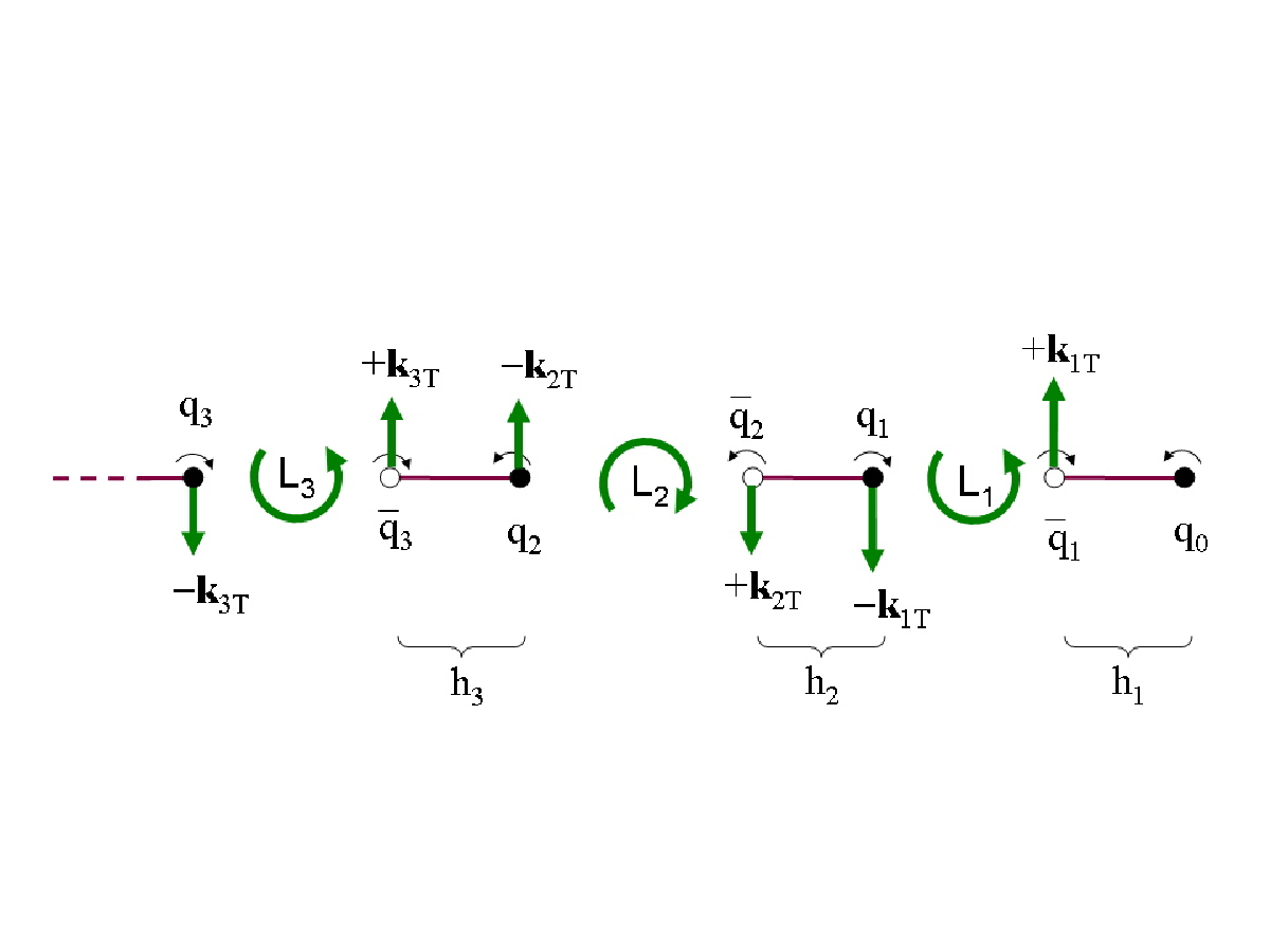
The Collins function for pions has been computed in various fragmentation models [178, 179, 180, 181, 182]. What is common to these approaches is that arises from the interference between a tree level amplitude and loop corrections that provide the necessary imaginary parts. The differences reside in the pion-quark couplings and in the nature of the virtual particles in the loops (pions or gluons). An assessment of model calculations of the Collins function is contained in Ref. [183].
4 Processes and observables related to transverse spin
In this section we will present a general description of the processes probing the transverse-spin and transverse-momentum structure of hadrons, and of the relevant observables: single-spin asymmetries, double-spin asymmetries and unpolarised azimuthal asymmetries. The focus will be on two classes of reactions that have clear and well-established theoretical descriptions, namely SIDIS with the related process annihilation into hadron pairs, and DY production. Hadroproduction will also be described, but in lesser detail. The last subsection contains a sketchy presentation of other processes somewhat related to transverse spin.
4.1 Semi-inclusive deep inelastic scattering (SIDIS)
SIDIS is the process , where () is the incoming (outgoing) lepton, the nucleon target, the detected hadron. The corresponding four-momenta are given in parentheses. In the following we will denote by and the longitudinal and transverse component of the target spin vector, respectively, and by the longitudinal polarisation of the incident lepton.
SIDIS is usually described in terms of the invariant variables , , , with and . In the deep inelastic limit, is much larger than the mass of the nucleon and the mass of the final hadron. Hereafter mass corrections are neglected unless otherwise stated.
To parametrise the cross section in terms of structure functions the so-called “ collinear frame” [184] is usually adopted. As shown in Fig. 11 in this reference frame the virtual photon and the target nucleon are collinear and directed along the z axis, with the photon moving in the positive direction, and the final hadron has a transverse momentum . All azimuthal angles are referred to the lepton scattering plane: is the azimuthal angle of the hadron , is the azimuthal angle of the nucleon spin vector . The phase space of the process contains another angle, , which is the azimuthal angle of the outgoing lepton around the beam axis with respect to an arbitrary fixed direction, which is chosen to be given by the target spin. Up to corrections of order one has [185].

In this Section we consider the case of a spinless or unpolarised detected hadron, while leptoproduction of transversely polarised hadrons will be treated in Section 4.1.4. The SIDIS differential cross section in the six variables and , is given by
| (56) |
where is the usual DIS leptonic tensor and is the hadronic tensor
| (57) | |||||
Neglecting for simplicity the corrections the complete SIDIS cross section can be parametrised in terms of 18 structure functions as follows [185, 126];
| (58) |
The structure functions depend on and . Their first and second subscript denote the polarisation of the beam and of the target, respectively ( = unpolarised, = longitudinally polarised, = transversely polarised), whereas the third subscript refer to the polarisation of the virtual photon.
If we integrate (58) over , only 5 structure functions survive: , and . The first two, upon a further integration in and a sum over all outgoing hadrons, yield the unpolarised DIS structure functions and . The second two lead to combinations of the structure functions and of longitudinally polarised DIS. The fifth one vanishes. The fact that
| (59) |
is a consequence of time-reversal invariance [185] and is another way to express the Christ-Lee theorem [26], according to which there cannot be transverse spin asymmetries in inclusive DIS. On the contrary, in SIDIS no first principle forbids the existence of transverse spin asymmetries.
In the literature, the spin and azimuthal asymmetries of SIDIS are defined in two different ways:
- -
as the structure function ratios:
(60) where and label the polarisation of the beam and of the target respectively, is a trigonometric function of its arguments, and ;
- -
as the azimuthal moments of cross sections [184]:
(61) where is a shorthand notation for the fully differential cross section.
Notice that the two definitions of asymmetries differ for -dependent factors.
4.1.1 SIDIS in the parton model
In the parton model the virtual photon strikes a quark (or an antiquark), which successively fragments into a hadron . The process is represented by the diagram in Fig. 12. We will take transverse momenta of quarks into account and refer to this description as the “extended parton model”.
For the partonic description of SIDIS we work in a reference frame where the momenta of the target nucleon and of the outgoing hadron are collinear and define the longitudinal direction. In this “ collinear frame”, one has and , whereas the virtual photon momentum acquires a transverse component . The incoming quark momentum is , with ; the fragmenting quark momentum is , with . Notice that the “transverse” quantities in the frame (labelled by the subscript ) differ from the “perpendicular” quantities in the frame (labelled by the subscript ) by terms suppressed at least as . In particular, is related to by , up to corrections.
The hadronic tensor corresponding to Fig. 12 is given by
| (62) | |||||
where the second expression has been obtained by working out the momentum-conservation delta function and neglecting terms. In this case one has and .
Inserting the expressions of and into (62) and contracting with leads to the SIDIS structure functions. With the following notation for the transverse momenta convolutions
| (63) |
the non vanishing structure functions at leading twist are [48, 50, 126]
| (64) | |||||
| (65) | |||||
| (66) | |||||
| (67) | |||||
| (68) | |||||
| (69) | |||||
| (70) | |||||
| (71) |
where . The structure function gives the dominant contribution to the unpolarised cross section integrated over .
The Collins term couples the Collins function to the transversity distribution , thus representing one of the privileged ways to access this quantity. Note that in the original paper [29] the Collins angle was defined as the angle between the momentum of the produced hadron and the spin of the fragmenting quark, i.e. . In terms of the azimuthal angle of the target spin , one has . On the other hand, according to the conventions of Ref. [184], the Collins angle is defined as . Thus, one gets different signs for the Collins asymmetry, depending on which definition of the Collins angle, either or , is adopted.
Another leading-twist asymmetry source is the Sivers term , which couples the Sivers function to the unintegrated unpolarised fragmentation function . In the transversely polarised case, a further angular modulation, of the type , involves the distribution function .
In unpolarised SIDIS, a leading-twist azimuthal asymmetry is generated by the structure function , which couples the Boer-Mulders distribution to the Collins fragmentation function .
Going to twist three, i.e. to order , it turns out that the leading-twist structure functions (64-70) do not acquire any extra contribution, but there appear other non vanishing structure functions [126]. Among them, of particular phenomenological importance are those related to the and modulations. Ignoring, in the spirit of the parton model, interaction-dependent terms, i.e. quark-gluon correlations, and quark mass contributions (the generalised Wandzura–Wilczek approximation) one finds [126]
| (72) | |||||
| (73) |
In the same approximation one gets . Thus a deviation of the beam-spin asymmetry from zero might signal the relevance of interaction effects in the nucleon. One should recall however that at high transverse momenta is non zero in next-to-leading order QCD. The term in containing the product of the unpolarised functions is a purely kinematical contribution arising from the intrinsic transverse motion of quarks, with no relation to spin. This contribution was discovered longtime ago by Cahn [186, 187], and the corresponding azimuthal asymmetry is referred to as the “Cahn effect”. A similar contribution emerges at twist four, that is at order , in the term:
| (74) |
All the above parton-model results have been obtained using the most general decompositions of the correlation matrices and , and inserting them into the SIDIS hadronic tensor . There is an alternative approach, which relies on the helicity formalism and expresses the cross section as a convolution of helicity amplitudes of elementary subprocesses with partonic distribution and fragmentation functions, taking fully into account non collinear kinematics [188]. Considering for simplicity an unpolarised lepton beam and a spinless or unpolarised final hadron, and adopting the collinear frame, the basic factorisation formula for the SIDIS cross section in this picture is, up to order ,
| (75) |
where the ’s are helicity indexes, is the probability of finding a quark with momentum fraction and transverse momentum inside the target nucleon, is the helicity density matrix of the quark , is the fragmentation function of the struck quark into the hadron with transverse momentum with respect to the fragmenting quark, and is the cross section of lepton-quark scattering at tree level. Note that, whereas in the collinear case the produced hadron is constrained to have and the entire process takes place in the scattering plane, the intrinsic transverse momentum of quarks introduces a non planar geometry. The elementary scattering amplitudes ’s take into account this non collinear and out-of-plane kinematics. Neglecting contributions, no Jacobian factors appear in eq. (75) and one has .
Despite their apparent dissimilarity, the two parton model approaches described so far, namely the approach based on quark correlation matrices and eq. (62) and the approach based on the helicity formalism and eq. (75), are equivalent as far as parton interactions are ignored. In other terms, all the leading-twist asymmetries listed in eqs. (64-71) can be exactly reobtained from eq. (75) [189], whereas at twist three the results of the two approaches are identical if one neglects the “tilde” distribution and fragmentation functions arising from quark-gluon correlations.
4.1.2 TMD factorisation in QCD
So far, we have only considered the extended parton model, i.e. the parton model incorporating intrinsic transverse momenta. One may wonder whether the results we have presented have any solid QCD foundation. The answer to this question is positive, at least in a particular kinematic regime. Semi-inclusive processes are characterised by two scales, besides the confinement scale : the momentum transfer and the transverse momentum of the final hadron or, equivalently, the transverse momentum of the virtual photon in the collinear frame.
Extending the pioneering work on back-to-back jet production of Ref. [89], a TMD factorisation theorem for SIDIS and DY has been proven [52, 51, 190]. The proof is valid in the low transverse-momentum region . In this framework the unpolarised SIDIS structure function is written as
| (76) | |||||
For simplicity the dependence of the distribution functions on and of the fragmentation function on ( and are vectors off the light-cone) is omitted . The variables and serve to regulate the light-cone singularities, as explained in Section 3.3. is a perturbative hard factor written as a series in powers of . The soft factor arises from the radiation of soft gluons (of transverse momentum ) and is a matrix element of Wilson lines in the QCD vacuum. Also not displayed in eq. (76) is the dependence of all quantities on the renormalisation scale and on the soft-gluon rapidity cut-off . Of course, the physical observable does not depend on any of these regulators.
4.1.3 QCD description at high transverse momenta

At high transverse momenta, , SIDIS structure functions can be described in collinear QCD. The azimuthal angular dependence of hadrons in leptoproduction was proposed longtime ago as a test of perturbative QCD [193]. In collinear factorisation, transverse momenta are generated by gluon radiation. At first order in the hard elementary processes shown in Fig. 13 contribute to the four unpolarised SIDIS structure functions and to the two double-longitudinal structure functions . Introducing the partonic variables and , defined as , , where and are the four-momenta of the incident and fragmenting partons, respectively, and and are the usual light-cone momentum fractions, i.e. and , one has for the ’s at leading order in and leading twist [194, 195, 192]
| (77) |
and analogous formulae for the ’s. The Wilson coefficients represent elementary cross sections and are listed in Ref. [192].
The structure function encountered in Section 4.1.1, which produces a beam-spin asymmetry and vanishes in the parton model, gets a non zero perturbative QCD contribution at leading twist and order [196, 197].
On the contrary, the transversely polarised structure functions , which vanish at leading twist in collinear factorisation, since there is no chirally-odd fragmentation function, emerge at twist three, as the result of quark-gluon correlations. Following the early work of Ref.[17, 18, 198], a twist-three collinear factorisation theorem valid at large transverse momenta was proven [53, 54, 55]. In this approach the cross section for SIDIS with a transversely polarised target has the general form [191, 199, 200]
| (78) |
where the first term contains a quark-gluon correlation function for the transversely polarised nucleon and the ordinary unpolarised fragmentation function for the final hadron, whereas the second term combines the transversity distribution with a twist-three fragmentation function. Let us focus on the first contribution (twist-three effects in the initial state). The hadronic tensor can then be written as
| (79) |
where the partonic tensor contributing to the transversely polarised structure functions is (see Fig. 14)
| (80) |
In this expression is the quark-gluon correlation matrix
| (81) |
and represents the perturbatively calculable partonic hard scattering. By means of the collinear expansion [54] one can get
| (82) |
and finally end up with
| (83) |
where the quark-gluon correlation matrix , defined as
| (84) |
contains the multiparton distributions introduced in Section 3.4. It is easy to verify that, due to the structure of , the hadronic tensor receives contributions only from the imaginary part of the hard blob, arising from internal propagator poles.
Considering for definiteness the Sivers contribution to the cross section, its explicit expression is [191, 199]
| (85) | |||||
The first two terms represent the so-called “soft-gluon pole” contribution (), the third term is the “soft-fermion pole” contribution (), the fourth term is the “hard pole” contribution (). The dots represent the contributions of and of the gluonic correlation functions.
In the intermediate transverse-momentum region, i.e. , one expects that both the TMD and the twist-three pictures should hold. This has been explicitly verified in Refs. [56, 58]. The output of these important works is a set of relations that connect the -odd TMD distributions (Sivers and Boer-Mulders functions) on one side, with the quark-gluon correlations on the other side.
4.1.4 Leptoproduction of transversely polarised spin baryons
The leptoproduction of spin baryons in another interesting channel to access transversity. If the nucleon target and the detected hadron are both transversely polarised, , the spin transfer between the initial and the final particle occurs in collinear kinematics. The cross section integrated over the transverse momentum gets in fact a double-spin term proportional to the product of the transversity distribution and the “transversity” fragmentation function .
This doubly polarised process has the advantage of being free from the theoretical complications related to the transverse motion of quarks: the ordinary collinear QCD factorisation theorem applies and a perturbative study is possible, since we know the evolution of both (Section 3.2) and [201]. At leading order in QCD, the transverse polarisation of the produced baryon is given by
| (86) |
where is the nucleon polarisation and is the spin transfer coefficient of quarks.
In the case of hyperons, information on the spin transfer in the fragmentation process can be obtained from the polarisation extracted from the angular distribution in the weak decay. The transverse polarisation of ’s produced in hard processes with initial transversely polarised hadrons was studied long time ago in Refs. [202, 203], and reinvestigated more recently [204, 32]. Phenomenological analyses are presented in Refs. [205, 206, 207]. The transversity fragmentation function is measurable in production of transversely polarised pairs.
Transverse polarisation can also be observed in SIDIS with an unpolarised target, by measuring asymmetries in the transverse momentum distribution of the hyperons. One contribution (-odd in the final state) involves the quark density and the polarising fragmentation function . This mechanism for polarisation in SIDIS was studied in Ref. [208]. Another contribution (-odd in the initial state) involves the Boer-Mulders function coupled to the (unintegrated) fragmentation function . At high , this effect has a counterpart in the twist-three approach. The initial-state -odd mechanisms for producing polarisation have been investigated in the context of twist-three factorisation by Zhou, Yuan and Liang [209].
4.1.5 Two-hadron leptoproduction
Another partially inclusive DIS reaction that can provide information on the transverse-spin structure of hadrons, and in particular on transversity, is two-particle leptoproduction from a transversely polarised target, , with the two spinless final hadrons in the same jet. Two-hadron production in SIDIS has been proposed and studied by various authors [210, 33, 211, 212] as a process probing the transverse polarisation distribution in combination with a dihadron fragmentation function (DiFF). The idea is to look at an angular correlation between the spin of the fragmenting quark and the relative transverse momentum of the hadron pair, without involving the transverse momenta of quarks. Integrating over the total transverse momentum of the final hadrons, one gets an asymmetry in the azimuthal angle between the two-hadron plane and the scattering plane. This asymmetry is determined by a fragmentation function usually called , which does not depend on the intrinsic transverse motion of quarks and arises from the interference between different channels of the fragmentation process into the two-hadron system. Thus, all the difficulties related to non-collinearity are in this process avoided.
The first authors who suggested resonance interference as a way to produce non-diagonal fragmentation matrices of quarks were Cea et al. [213] in their attempt to explain the observed transverse polarisation of hyperons produced in interactions [4]. The unpolarised dihadron fragmentation functions appeared for the first time in the context of jet calculus [214, 215]. The extension to the polarised case was discussed in Refs. [210, 30, 216, 33] and a complete classification of the DiFF’s was given at leading twist in Ref. [211] and at twist-3 in Ref. [217].
The kinematics of the process in the frame is shown in Fig. 15. We introduce the total momentum of the hadron pair (with invariant mass ), the relative momentum , and the variables (the light-cone fraction of the fragmenting-quark momentum carried by the hadron pair) and (which describes how the total momentum of the pair is split into the two hadrons). is the transverse component of with respect to , and is the azimuthal angle of in the plane orthogonal to the axis, measured with respect to the scattering plane. The azimuthal angle of the target spin vector is . Calling the transverse momentum of the fragmenting quark with respect to , the unpolarised and transverse-spin projections of the two-hadron fragmentation matrix at leading twist are
| (87) | |||
| (88) |
These are the probabilities for an unpolarised quark and for a transversely polarised quark, respectively, to fragment into a hadron pair. Upon integration over , the contribution of the Collins-type DiFF disappears, and the only remaining transverse-spin term is the one containing the (integrated) interference fragmentation function .

It is convenient to consider the centre-of-mass frame of the two hadrons (Fig. 15), where and is the angle between the direction of the hadron emission and (in the frame). For two alike hadrons of mass , one has and . In terms of these variables, keeping only the unpolarised and the transversely polarised terms, the leading-twist partonic expression for the cross section of two-hadron leptoproduction reads
| (89) | |||||
Here it is , a relation valid modulo corrections. At twist three, there appear extra terms in the cross section: a unpolarised contribution and a transverse-spin contribution [217].
The first model for the two-pion DiFF was presented in Ref. [33], where the phase difference between and waves was taken from phase shifts in elastic scattering. The resulting fragmentation function (called in Ref. [33]), changes sign around the mass.
In a more recent model [218] the fragmentation functions are expanded in Legendre polynomials of keeping only the first few terms, corresponding to the lowest values of relative orbital momentum. This truncation is expected to be legitimate for not very large . Thus one can write
| (90) | |||
| (91) |
(remember that multiplies a factor in the cross section). The interpretation of these terms, signaled by their superscripts, is the following [218]: is a diagonal component, receiving contributions from and waves of the dihadron system separately (the “background”); and originate from the interference of a wave and a wave; and arise from the interference of two waves. The main channels contributing to the fragmentation of a quark into a pair are: 1) incoherent fragmentation, ; 2) fragmentation via a resonance, ; 3) fragmentation via a resonance decaying into three pions, . Pions in channel 1 are expected to be mostly produced in wave; pions in channel 2 come from the two-body decay of a vector meson and are in a relative wave; pions in channel 3 are prevalently in wave, but a fraction of them may also be in wave. The functions and arise from the interference of channels 1-2 and 1-3 [219].


A model based on a more sophisticated analysis of the fragmentation channels [219] predicts a completely different behaviour for , with a peak at the mass and a broader maximum at the mass. Its size is about 30 % of the unpolarised fragmentation function as shown in Fig. 16.
A different definition of the relative transverse momentum is proposed by Artru [28], who uses the vector , which is perpendicular to the axis, and its azimuthal angle . The advantage of is that it is by construction invariant with respect to boosts along the direction, which is not the case of although the two angles are the same in the frame. Using the recursive fragmentation string model (see Section 4.1.5) the “joint spectrum” of the first and the second rank hadrons has been calculated [177]. By suitably integrating the spectrum, expressions for both the Collins FF and the dihadron FF in principle may be obtained.
4.2 Inclusive production of hadron pairs in annihilation
An independent source of information on the Collins fragmentation function is inclusive two-hadron production in electron–positron collisions, , with the two hadrons (typically pions) in different hemispheres. We know that the Collins function produces a modulation, where is the azimuthal angle between the plane containing the quark and the hadron momenta, and the plane normal to . Considering a single jet in hadron production, the Collins modulation would average to zero in a large event sample. Thus, in annihilation the Collins effect can only be observed in the combination of two fragmenting processes of a quark and an antiquark, resulting in the product of two Collins functions with an overall modulation of the type , where and are the azimuthal angles of the final hadrons around the quark-antiquark axis, with respect to the scattering plane.
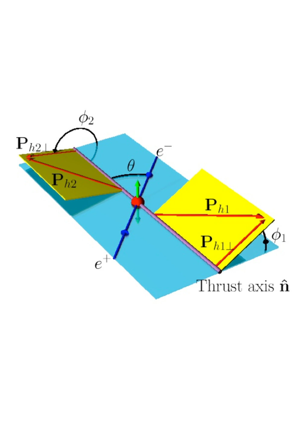
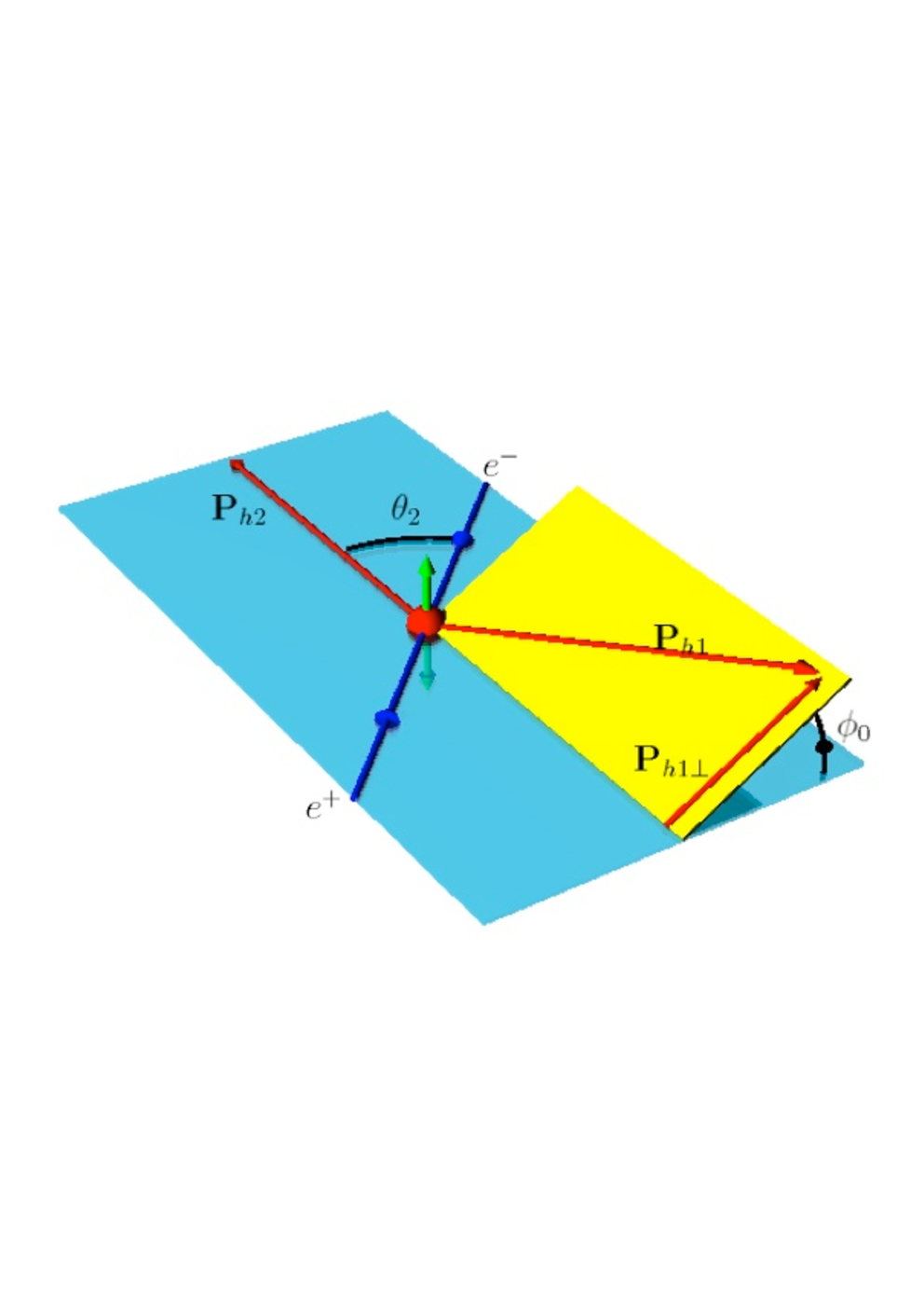
Two-hadron production in collisions was studied in Refs. [220, 221, 222, 223, 224, 225]. The tree-level differential cross section in the jet frame with respect to the quark-antiquark direction (Fig. 17, left) reads
| (92) | |||||
where ( is the angle between the lepton axis and the axis, in the centre-of-mass frame, whereas gives the orientation of the scattering plane around the axis), and we have introduced the one-dimensional moments
| (93) |
Eq. (92) and the following results refer to the case of photon-mediated annihilation. production and interference effects have been investigated in Refs. [222, 225].
From an experimental point of view, the quark-antiquark direction is not directly accessible, and is approximated by the dijet thrust axis , defined by
| (94) |
where the sum is over all detected particles. The resulting asymmetry is given by
| (95) |
We will refer to this method of extracting the Collins asymmetry by measuring azimuthal distributions around the thrust axis as to the “ method” [221, 44, 226, 225].
There is another way of reconstructing the asymmetry, the so-called “ method”, which is based on a different geometry and does not require the knowledge of the thrust axis. In this case one measures the hadron yields as a function of , the angle between the plane containing the momentum of hadron 2 and the leptons, and the plane defined by the two hadron momenta [222, 223, 225] (this frame, shown in Fig. 17 (right), is similar to the Gottfried-Jackson frame in Drell-Yan processes [227]). The corresponding cross section is
| (96) |
where and are the transverse momenta of the two fragmenting quarks with respect to the hadron directions. The asymmetry reads
| (97) |
Electron-positron scattering can also allow accessing the fragmentation function of transversely polarised baryons [27, 220, 228]. In the case of ’s, the specific process is back-to-back inclusive production, , with the hyperon and the anti-hyperon decaying into and , respectively. It was shown in Ref. [220] that the cross section of this process contains an azimuthal modulation proportional of the type , where is the angle between the collision axis and the axis in the jet frame (Fig. 17, left) and are the azimuthal angles of the proton and antiproton in the same frame (with the direction given by the jet and the axis in the plane of the beams and jets. The asymmetry is determined by measuring the difference between the number of pairs on the same side of the scattering plane and the number of pairs on opposite sides.

Finally, the interference fragmentation function can be extracted from the production of two hadron pairs in electron-positron annihilation: , where the particles in brackets belong to two back-to-back jets [216]. The (complicated) geometry of this process is shown in Fig. 18. The observable quantity is the angular correlation of the production planes, expressed by the so-called Artru-Collins asymmetry. The kinematics of the process is described by doubling the variables introduced in Section 4.1.5. If we call and the azimuthal angles of the transverse relative momenta and of the two hadron pairs, the Artru-Collins azimuthal asymmetry is the correlation.
In annihilation, the interference fragmentation functions and the Collins function are typically probed at much larger scales compared to SIDIS. However, the evolution of , differently from that of , is known [229]. Therefore, a consistent combined analysis of dihadron production in annihilation and SIDIS is possible and may provide an alternative way to extract the transversity distributions [230].
4.3 Drell-Yan production
Drell-Yan (DY) dilepton production with various polarisations of the two particles in the initial state is a very rich source of knowledge on the hadronic structure. The main advantage of this class of reactions is that they do not involve fragmentation functions, but only parton distributions. However, unless one considers antiproton–proton scattering, or pion-proton scattering, DY processes necessarily involve sea valence products. This means that, while they provide direct information about antiquark distributions, which are less determined in SIDIS, their asymmetries are generally small.
In principle, DY production with two transversely polarised hadrons is the cleanest reaction for studying the transversity distribution and the pioneering works of Ref. [25] and [231] were indeed devoted to this process. However, in order to observe sizable double-spin asymmetries and extract , we probably have to wait for a new generation of experiments with polarised antiprotons [232]. On the other hand, unpolarised and singly-polarised DY processes can probe a large variety of TMD’s related to transverse spin, and are now attracting a wide theoretical and experimental interest.
4.3.1 Kinematics and observables
Drell-Yan lepton-pair production is the process , where and are hadrons and is an undetected system. The center-of-mass energy squared of this reaction is , having neglected in the approximate equality the hadron masses and . The lepton pair originates from a virtual photon with four-momentum . In contrast to DIS, is a time-like vector: , and the invariant mass of the lepton pair coincides with . The deep inelastic limit corresponds to , with fixed and finite.
The DY cross section is usually expressed in a dilepton center-of-mass frame and can be written as
| (98) |
where is the familiar leptonic tensor and is the DY hadronic tensor. Among the infinite dilepton c.m. frames, related to each other by a rotation, the most often used is the Collins-Soper (CS) frame [233], characterised by a z axis that bisects the angle between and as shown in Fig. 19. Another common dilepton c.m. frame is the Gottfried–Jackson frame [227], where the axis coincides with the direction of one of the colliding hadrons.

In the unpolarised case the DY hadronic tensor contains four independent structure functions [234]. Using the classification of Ref. [235] the cross-section becomes
| (99) |
The double subscript refers to the polarisation states of the two colliding hadrons: = unpolarised, = longitudinally polarised, = transversely polarised. In literature [234], the structure functions are also called (apart from a common factor), , respectively. The angular distribution of leptons is often parametrised as
| (100) |
The three quantities , and are related to , and by
| (101) |
The so-called Lam-Tung relation [234, 236, 237]
| (102) |
which corresponds to , is valid at order in collinear QCD [238] (see below) and is slightly violated at order [239].
In the polarised case, a complete analysis of the DY hadronic tensor is contained in Ref. [235], where it is shown that in single-polarised DY, first studied in [231], the number of independent structure functions is 16, whereas the double-polarised hadronic tensor contains 28 structure functions, so that altogether the number of independent structure functions in DY is 48. The full cross section can be found in Ref. [235]. Limiting ourselves to unpolarised, single-transverse and double-transverse contributions, the cross section reads
| (103) |
and are the azimuthal angles of the spin vectors of hadrons and , respectively. This angular structure is valid in any dilepton c.m. frame, but the numerical values of the structure functions are frame-dependent.
In the parton model and at leading order in QCD the two invariants and can be interpreted as the fractions of the longitudinal momenta of the hadrons and carried by the quark and the antiquark that annihilate into the virtual photon. In the c.m. frame of the two colliding hadrons, which is the most convenient frame to study the partonic structure of the hadronic tensor, the photon momentum can be parametrised as and acquires a transverse component . Neglecting terms of order , one has , that is . The structure functions in eq. (103) can be expressed in terms of the four variables .
Other variables customarily used are the rapidity of the virtual photon, and the Feynman variable . In a dilepton c.m. frame, . The relation between and is . The DY cross-section can be variously reexpressed in terms of these variables:
| (104) |
4.3.2 DY asymmetries in the TMD approach
In the parton model, calling and the momenta of the quark (or antiquark) coming from hadron and respectively, the hadronic tensor shown in Fig. 20 is
| (105) |
Here is the quark correlation matrix for hadron , is the antiquark correlation matrix for hadron , and the factor has been added since in and summations over colours are implicit. It is understood that, in order to obtain the complete expression of the hadronic tensor, one must add to (105) a term with replaced by and replaced by , which accounts for the case where a quark is extracted from and an antiquark is extracted from . In the following formulae we shall denote this term symbolically by .

Introducing the longitudinal momentum fractions and , and working out the delta function of four-momentum conservation, one finds , and the hadronic tensor becomes
| (106) |
Inserting here the explicit partonic expressions of the quark correlators, it is not difficult to get the parton model expressions of the DY structure functions [47, 240, 235]. Only 24 of these 48 structure functions are non vanishing at leading twist. The most relevant ones are, in the Collins-Soper frame (but the Gottfried-Jackson expressions differ from these only by subleading terms )
| (107) | |||
| (108) | |||
| (109) | |||
| (110) | |||
| (111) |
where and denotes the transverse-momentum convolution of eq. (63) with the addition of the term. In eq. (110) we defined the combinations and , which correspond to the angular modulations indicated by their superscripts.
Eqs. (107-111) contain a series of interesting results. First of all, the Boer-Mulders function generates a asymmetry in unpolarised DY. At leading twist, the parameter is given by
| (112) |
Since and , the Lam-Tung relation is violated, and this is one of the remarkable consequences of the intrinsic transverse motion of quarks.
Concerning singly-polarised Drell-Yan processes, the Boer-Mulders function combines with the transversity distribution in the , or , asymmetry, whereas the Sivers function is probed via the (or ) structure function associated with the (or ) asymmetry. Note that upon integration over the lepton angles only the Sivers asymmetry is non vanishing.
4.3.3 DY double transverse asymmetries
With two transversely polarised colliding hadrons, the term provides a direct access to transversity. Inserting eqs. (107, 111) into eq. (103) and integrating the cross section over , one gets
| (113) | |||||
This parton-model expression can be generalised to QCD by resorting to the collinear factorisation theorem, which for the polarised DY process reads [241]
| (114) |
where and are the momentum fractions of the quark (from hadron ) and antiquark (from ), and are the quark and antiquark spin density matrices, is the cross-section matrix of the elementary subprocesses in the quark and antiquark helicity space, is the factorisation scale. At leading order, i.e. , the only contributing subprocess is and , . In the transversely polarised case, one reobtains eq. (113), except that all distribution functions acquire a -dependence. Thus the LO double transverse asymmetry is
| (115) |
where
| (116) |
is the elementary double-spin asymmetry for . We see that a measurement of would directly provide the product of quark and antiquark transversity distributions, with no mixing with other unknown quantities. At next-to-leading order (NLO) the DY transverse cross section gets contributions from virtual-gluon (vertex and self-energy) corrections and real-gluon emission, which were calculated by several authors with different methods [242, 243, 244, 81]. The NLO double transverse asymmetry was investigated in Refs. [245, 246, 247, 248].
4.3.4 DY azimuthal and spin asymmetries in QCD
As in the case of SIDIS, perturbative gluon radiation can generate a non-zero transverse momentum . For instance, the contribution of the quark-antiquark annihilation process to the unpolarised angular distribution in the Collins-Soper frame is [238]
| (117) |
where we have omitted the term which is the only one depending on the quark and antiquark distributions. From (117) one gets
| (118) |
and the Lam-Tung relation is fulfilled. The contribution of the is more complicated, but also satisfies the Lam-Tung relation, which holds for the complete leading-order cross section.
The perturbative QCD approach to the DY angular distribution sketched above holds for . At small , large logarithms of the form appear, which must be resummed. This is done in the space conjugate to and gives rise to a Sudakov form factor, according to the Collins-Soper procedure [89]. The Sudakov resummation for the structure functions of unpolarised DY production, including those related to azimuthal asymmetries, has been studied in Refs. [249, 250] and the Lam-Tung relation is found to be unaffected by the resummation.
The perturbatively generated asymmetry is suppressed as at small . A further contribution to this asymmetry can arise in the twist-three approach from the product of two quark-gluon correlation functions , one associated with the quark from hadron , the other with the antiquark from hadron [251].
In the singly-polarised DY case the situation is again analogous to SIDIS. At large , a DY single-spin asymmetry is generated by the quark-gluon correlator of the polarised hadron. A smooth transition from this twist-three mechanism to the Sivers effect occurs in the intermediate region , where both the higher-twist and the TMD factorisations apply [57]. Another SSA’s arises from the chirally-odd quark-gluon correlation function of the unpolarised hadron coupled to the transversity distribution of the transversely polarised hadron, but in the low limit this contribution vanishes (after integration over the lepton angles only the Sivers asymmetry survives).
4.4 Inclusive hadroproduction
We finally discuss a third class of reactions that probe the transverse-spin and transverse-momentum structure of hadrons: inclusive hadroproduction with one transversely polarised hadron in the initial state, that is , where an unpolarised (or spinless) hadron is produced with a transverse momentum with respect to the collision axis. An interesting variation of this process is the production of a transversely polarised hadron, i.e., a hyperon, from unpolarised hadron-hadron scattering, that is (Section 4.4.3). We will limit ourselves to a brief description of these reactions, referring the reader for more detail to some reviews [63, 252] and to the original papers.
We first consider hadroproduction with a transversely polarised colliding particle. The measured quantity is the single-spin asymmetry
| (119) |
with the cross sections usually expressed as functions of and of the Feynman variable ( being the longitudinal momentum of the produced hadron). In terms of the scattering angle , Feynman’s can be written as . Another often used variable is the pseudorapidity .
According to the QCD factorisation theorem [253, 241] the differential cross-section for hadroproduction at large can be formally written as
| (120) |
Here () is the distribution of parton () inside the hadron (), is the spin density matrix of parton , is the fragmentation matrix of parton into hadron , and is the (perturbatively calculable) cross-section of the elementary process (a two-body scattering, , at lowest order).
If the produced hadron is unpolarised, or spinless, only the diagonal elements of are non zero, i.e. , where is the unpolarised fragmentation function. Together with helicity conservation in the partonic subprocess, this implies . Therefore, the cross section (120) carries no dependence on the spin of hadron and all single-spin asymmetries vanish [16]. In order to escape such a conclusion one must consider either the intrinsic transverse motion of quarks [34, 29, 30], or higher-twist effects [17, 18, 198, 19, 53, 54]. In the former case, one can probe a number of distribution and fragmentation functions, including the transversity distribution (transversely polarised quarks in hadron ), the Sivers function (unpolarised quarks in hadron ), the Boer-Mulders function (transversely polarised quarks in hadron ), the Collins function (transversely polarised quarks fragmenting into hadron ). The twist-three single-spin asymmetries involve various quark-gluon correlators, either in the initial state (distribution functions), or in the final state (fragmentation functions). The main problem is that all TMD or twist-three contributions mix up in a single observable, , which makes the physical interpretation of the results quite unclear.
4.4.1 Hadroproduction in the extended parton model
When the intrinsic transverse motion of quarks is taken into account, the QCD factorisation theorem for inclusive hadroproduction is not proven, and actually is known to be explicitly violated in some cases [254, 104]. Nevertheless, one can write a non-collinear factorisation formula in the context of the extended parton model, with a tree-level elementary kernel. One must obviously recall that: i) the generalisation of this kernel to higher order in is not a legitimate procedure; ii) the transverse-momentum dependent distribution and fragmentation functions appearing in the hadroproduction factorisation formula are not guaranteed to be universal quantities, i.e., to be the same functions as in other processes.
The extended-parton model formula generalising eq. (120) is (we consider the production of a spinless hadron) [188]
| (121) |
where the convolutions are now not only on the longitudinal momentum fractions , but also on the transverse momenta . Note that even though is unpolarised, its -dependent fragmentation matrix is non diagonal. The elementary cross sections have the structure . The amplitudes refer to the elementary subprocess (remember that we are considering the tree level only). A natural reference frame is the center-of-mass frame of the colliding hadrons. The collision axis forms with the direction of the produced hadron a plane, that we call the hadronic plane. The tricky point about eq. (121) is that, due to intrinsic transverse momenta, the partonic scattering does not take place in the hadronic plane. This non-planar geometry gives rise to some non-trivial phases in the distribution and fragmentation matrices. Also, the amplitudes appearing in eq. (121) must be Lorentz transformed to the canonical amplitudes defined in the partonic center-of-mass frame, an operation which introduces further phases. This complicated structure has been fully worked out in Ref. [188], where all the details concerning the kinematics and the scattering amplitudes can be found. Here we limit ourselves to quoting some general results. The contribution to the transverse single-spin asymmetry from the subprocess schematically reads
| (122) | |||||
One recognises the Sivers effect (first term), the Collins effect (second term), the Boer-Mulders effect (third term) and a mixed effect (fourth term). The other contributions, , , , , , , , are explicitly given in Ref. [188]. They contain, besides the distributions and fragmentation functions of linearly polarised gluons, the gluon Sivers function . For instance, the and contributions are
| (123) |
Processes that select these terms and allow accessing the gluon Sivers function are meson production (which is dominated by the channel) [255] and pion production at midrapidity (which probes in the RHIC kinematics the small region and thus proceeds predominantly via gluonic channels) [256]. Other reactions probing the Sivers functions of quarks and/or gluons without contributions from the fragmentation sector are prompt-photon production [257, 258, 259], photon–jet production [258, 260], back-to-back dijet production [261].
On the contrary, the Collins effect can be singled out by studying asymmetric azimuthal correlation of hadrons inside a jet, that is [262].
4.4.2 Single-spin asymmetries at twist three
As pointed out in Ref. [17, 198], non-vanishing single-spin asymmetries can be obtained in perturbative QCD at higher-twist level. A twist-three factorisation theorem was proven for direct photon production [53, 54] and hadron production [55]. This work has been extended to cover the chirally-odd contributions [263, 264, 265]. Here we limit ourselves to quoting the main general results of these works. The twist-three phenomenological studies of data is treated in Section 5.5.
At twist three the hadroproduction cross section is formally given by
| (124) | |||||
where and are the quark–gluon correlation functions introduced in Section 3.4, is a quark–gluon correlator in the fragmentation process and , and are cross-sections of hard partonic subprocesses. The first term in (124) corresponds to the chirally-even mechanism considered by Qiu and Sterman [55]. The second term is the initial-state chirally-odd contribution analysed in Ref. [263]. The third term is the final-state contribution studied in Ref. [266]. The details and the elementary cross-sections can be found in the original papers.
4.4.3 production
The origin of the large transverse polarisation of hyperons measured since the 70’s [4, 5] in high-energy unpolarised hadron-hadron scattering is a longstanding problem (for reviews see Refs. [267, 268]). A transverse-momentum mechanism able to produce sizable asymmetries in involves the polarising fragmentation function introduced in Section 3.8, which describes the fragmentation of an unpolarised quark in a transversely polarised hadron [174]. In the twist-three approach the polarisation is generated by the chirally-odd spin-independent quark-gluon correlation function [209].
While in the polarisation must vanish at pseudorapidity for symmetry reasons. in +jet production no such constraint exists. The process has been proposed as an alternative way of probing through the correlation between the transverse momentum and spin of the with respect to the dijet axis [269].
4.5 Other processes
We conclude our discussion of the transverse-spin effects in hard processes by listing a series of reactions that have been proposed as sources of information on transversity and TMD’s.
- -
- -
Dilepton photoproduction: . It has been shown [271] that the transverse SSA of this reaction involves the transversity distribution multiplied by the chiral-odd distribution amplitude of the photon.
- -
Exclusive electroproduction: . Using a model for the GPD’s and relating to the tensor charge, the authors of Ref. [272] show that the transverse-spin asymmetry of this process can provide information on the tensor charge .
- -
Photo- and electroproduction of two vector mesons: . If one of the mesons is transversely polarised this reaction probes the transversity GPD [273].
5 Experimental results and phenomenological analyses
In the last decade, many transverse-spin effects have been measured in SIDIS on transversely polarised targets mainly by the HERMES and COMPASS Collaborations, in hadron-hadron scattering by the RHIC spin experiments, and in unpolarised Drell-Yan processes at Fermilab.
In this section, we review some of the recent experimental findings together with their phenomenological interpretation. The selected data are organised according to the physics information they provide. We start with the measurements aiming to access the transversity distribution, including the related measurements which are being performed in collisions. Then we describe the experimental results related to the -odd TMD’s (Sivers and Boer-Mulders function) and we conclude this part with a brief discussion of some measurements involving the -even TMD’s and higher-twist PDF’s. The RHIC hadroproduction results cannot easily be fitted in this scheme, and are presented in a separate subsection.
Since most of the results currently used to access transversity and TMD’s come from the SIDIS experiments, we feel useful to give in section 5.1 some details on the kinematical ranges of the present SIDIS experiments and on the analyses these experiments are doing, which are essentially common to all the SSA’s extraction.
Note: Although one should in principle distinguish between the
longitudinal momentum fraction
and the Bjorken variable ,
we have seen that they coincide as far as corrections
are neglected.
For the sake of simplicity, in this section
we ignore this distinction and write the distributions as functions
of . Analogously, we take to be the the argument of
fragmentation functions.
In the data plots, obviously and always stay for
and and for .
Other notations:
is the transverse momentum of the initial quark and is the transverse momentum of the
produced hadron with respect to the fragmenting quark.
In SIDIS is the transverse momentum of the
final hadron with respect to the axis.
In hadroproduction
is the transverse momentum of the final
hadron with respect to the collision axis.
5.1 SIDIS kinematics and SSA extraction
The SIDIS events are usually identified with standard cuts, with some differences for the different channels and for the various experiments due to the different beam energies and thus to the different kinematical domain. The DIS events are selected requiring the photon virtuality to be larger than 1 GeV2. The fractional energy transfered from the beam lepton to the virtual photon has to be larger than 0.1, to remove events affected by poor energy resolution, and smaller than 0.9 (or 0.95), to avoid the region most affected by radiative corrections. A minimum value of invariant mass of the final hadronic state GeV is also needed to exclude the resonance region. Typically, values of larger than 4, 10 and 25 GeV2 are required in the data analyses of the JLab, HERMES and COMPASS experiments respectively.
The variables , and , for the selected events, cover ranges which strongly depend on the lepton beam energy. Fig. 21 shows the regions of the (, ) plane kinematically accessible with lepton beams of 160 GeV, 27.5 GeV and 6 GeV momenta, corresponding to the COMPASS, HERMES and JLab experiments respectively.

In the COMPASS experiment the range is between 0.004 and 0.3, where the upper limit is given by the low luminosity; for the HERMES experiment , while the JLab experiments can presently measure with high precision at , in the valence region. The average values are also different and there is a strong correlation. At the mean value is 6.4 GeV2 at COMPASS and about 2.5 GeV2 at HERMES, while at the values are about 20 GeV2 and 6.2 GeV2 respectively. In the overlap region the ratio of the mean values measured in the two experiments goes from 2 to 3 with increasing , in spite of the similar mean values when integrating over the whole range. The values are between 25 and 200 GeV2 for COMPASS, between 10 and 50 GeV2 for HERMES, and below 10 GeV2 for the present JLab experiments. The differences in the covered kinematical regions make the experiments complementary, and, all together, they guarantee a very good coverage of the phase space.
In addition to the requirements on the inclusive DIS variables, in the data analysis cuts on the energy final state hadrons are applied, which also depend on the experiment and on the physics channel under consideration. Particle identification implies momenta above the RICH thresholds, which depend on the detector used in the experiment. In the single hadron analyses, the relative energy of each hadron has to be between 0.2 and 0.8. The upper limit, usually not required in the COMPASS analyses, is chosen to reject exclusively produced hadrons. The lower limit is used to select hadrons from the current fragmentation region. To do that, a selection based on the hadron rapidity should be applied, or, equivalently, the so-called Berger criterion should be fulfilled. This criterion [274] has been tuned on unpolarised SIDIS data and allows to relax the request based on the value alone by asking for each hadron a large enough . Thus, if GeV, all hadrons belong to the current fragmentation. Going down to GeV only hadrons with belong to this region, while if GeV one should cut at to be safe.
The azimuthal asymmetries in SIDIS introduced in Section 4.1 are defined as
| (125) |
where is a trigonometric function of a linear combination of and , and refer to the beam and target polarisations (U, L, or T). The asymmetries can be extracted from the measured distribution of the final state hadrons in the relevant azimuthal angle . In the following, the methods used to evaluate the transverse SSA’s in the HERMES and in the COMPASS experiments will briefly described.
In principle, since all the trigonometric functions appearing in the cross-section are orthogonal, the amplitudes of the azimuthal modulations (the so-called “raw asymmetry” ) can be obtained as twice the mean value of , or by fitting the azimuthal distribution with a function of the type . In practice this procedure requires to correct the azimuthal distribution for possible acceptance effects by means of Monte Carlo simulations. This can be avoided in the case of the SSA’s by collecting data with two opposite spin orientations, indicated with “+” and “-” in the following. If the acceptance and the detector efficiencies are the same for the two sets of data, no Monte Carlo correction is needed when fitting the function on the quantities
| (126) |
Here are the numbers of events in a given bin, is the normalisation factor between the two sets of data, and is always measured assuming the same orientation of the target polarisation for both sets of data. In the case of the HERMES experiment, the target spin orientation is flipped every second, so that acceptance and overall efficiencies can safely be assumed to be the same for the two sets of data. In the case of the COMPASS experiment, in which the target polarisation can be reversed typically only after a few days of data taking, the target is divided in cells with opposite polarisation directions. This allows to minimise the possible systematic effects due to acceptance variations by using, instead of the so-called “ratio product” quantities [43] which combine the number of events from the different cells and with the different target polarisation orientation. These quantities do not dependent on the beam flux and on the acceptances, under the assumption that the relative variations are the same for all the target cells, and they have a very simple expression in terms of the azimuthal modulation one wants to extract.
The methods described above are simple and direct, still some systematic effect can be relevant. In particular, the apparatus acceptance can introduce correlations between the physical asymmetries. For this reason different and more elaborated methods have been developed, which include the binning of the data in the plane and the fit with a function which includes all the modulations which appear in the cross-section. In the most recent analyses, both HERMES [275, 276] and COMPASS [277, 278, 279] have introduced “unbinned” maximum-likelihood methods based on maximum-likelihood fits with the data unbinned in and . The probability distributions include all the expected azimuthal modulations, both for the spin independent and the transverse target spin dependent parts of the cross-section. The spin independent part turned out not to influence the results for the SSA’s. In the COMPASS case, the same is true for the acceptance of the apparatus, assumed to have the same relative variations for all the target cells [278], and the SSA’s obtained with the “unbinned” maximum-likelihood method are in very good agreement with those extracted from the simpler methods used previously.
In order to obtain the final results, here called SSA’s, the raw asymmetries obtained with such fits have to be divided by the target (and beam) polarisation. The result are the HERMES “moments” or “amplitudes”, usually indicated with . In the COMPASS data, the raw asymmetries are divided by the target polarisation, by its dilution factor , and by the kinematical -dependent factors, usually dependent on the experimental acceptance in . As an example, the Collins SSA’s published by COMPASS are obtained by dividing the raw asymmetries by the target polarisation, by the dilution factor , and by the mean value of the transverse polarisation transfer from the initial to the final quark in the elementary lepton-quark scattering . The HERMES results for the Collins asymmetry (the so-called “lepto-beam asymmetries”) are only divided by the target polarisation.
Concerning the evaluation of possible systematic effects, it has to be noted that, even if the methods described above allow to extract simultaneously all the SSA’s, the systematic uncertainties have to be evaluated independently for all the modulations, since they can be different. For this reason, the results are not usually published all at the same time.
A final remark concerns the measurements of the asymmetries as functions of different kinematical variables, typically , and . Since in the experiments there is a strong correlation, very few attempts have been done to measure the dependence of the asymmetries in the various bins, which would be better studied by comparing the results of the different experiments. Usually the SSA’s are measured binning the data alternatively in , or , and integrating on the other two variables. This extraction introduces some correlation between the data, which should be taken into account when fitting all the results in a global analysis. To avoid this problem, the HERMES Collaborations is doing multi-dimensional analysis, which are not yet possible in COMPASS, due to the limited statistics.
5.2 Accessing transversity
Today, the most direct information on transversity is coming from SIDIS measurements with transversely polarised targets, which are complementary to the DY experiments and have the advantage of allowing a flavor separation by identification of the final state hadrons.
Among the various SIDIS observables related to transversity, the measurements performed so far have provided data on three of them: the Collins asymmetry, the two-hadron asymmetry, and the polarisation. They will be presented in the following subsections, after a a brief description of the event and hadron selection.
5.2.1 Collins asymmetry in SIDIS
The main source of information on the transversity PDF’s is at present the Collins asymmetry, which couples to the Collins fragmentation function . The Collins asymmetry has been measured by the HERMES [41, 275] and by the COMPASS [42, 43, 280, 279] Collaborations.
Before describing these results, it has to be mentioned that the asymmetries measured by the two experiments differ for the already mentioned correction by the factor, applied by COMPASS only, and for the sign because of the different definition of the Collins angle . In HERMES following the so-called “Trento convention” [184] it is defined as , while in COMPASS the original definition [29] is used, as mentioned in Section 4.1.1.
The first signal for a non-zero Collins asymmetry came from HERMES in 2005 [41], when the results on the data collected with the transversely polarised target in 2002 were published. The asymmetry had values clearly different from zero in the valence region and of opposite sign for positive and negative pions, and this was the first evidence that both the transversity and the Collins FF had to be different from zero. An interesting feature of the HERMES results is that the size of the asymmetry turned out to be roughly the same for positive and negative pions. As suggested in Ref. [41], this result implied that the favoured () and the unfavoured () Collins fragmentation functions and should be of the same size. In fact, neglecting the sea contribution (the asymmetry is different from zero only in the valence region) the flavour structure of the Collins asymmetry for a proton target can be written as
| (127) |
Due to the weight factor given by the quark charge, the measured asymmetries are not sensitive to , thus the result implies that . This finding, unexpected at the time, can be understood [41] in the framework of the string model of fragmentation which in its most recent version [177] is described in Section 3.8.1. If a favoured pion forms at the string end created by the first break, a disfavoured pion from the next break will be opposite in charge and will inherit transverse momentum from the first break in opposite direction from that acquired by the first pion. Also, assuming that the and quark contributions add up in the asymmetries, in the same model it is expected that their transversity distributions have opposite sign.

The COMPASS experiment started data taking with the transversely polarised deuteron target, and the first results [42] were published almost at the same time as the HERMES results. The measured Collins asymmetries were all compatible with zero, both for positive hadrons and for negative hadrons. This result is compatible with the HERMES finding. Limiting again the analysis to the valence region, the deuteron asymmetries can be written as
| (128) |
The straightforward conclusion from the COMPASS deuteron measurements is that and must have roughly the same size and opposite sign, very much as in the case of the helicity quark distributions.
Both HERMES and COMPASS have continued the measurements with the proton and the deuteron targets respectively, and have produced results with considerably better statistics, which have confirmed the first measurements.
The HERMES results based on the whole data collected from 2002 to 2005 [281] are shown in Fig. 22 for pions (left) and charged kaons (right).
The applied cuts are GeV2, , GeV2 and all the hadrons with 2 15 GeV, 0.2 0.7, and a polar angle with respect to the direction of the virtual photon larger than 0.02 rad are used in the extraction of the asymmetries. In the figure the bands represent the maximal systematic uncertainty which includes hadron misidentification and acceptance and detector smearing effects, and is smaller than the statistical one. The scale uncertainty due to the target polarisation has been evaluated to be about 8%. The fraction of charged pions and charged kaons produced in vector meson decay has also been estimated. As can seen in the figure, the asymmetries for and have opposite sign, increase from very small values at to about 5% at the highest values, and have a similar magnitude. The asymmetries are compatible with zero.

The COMPASS results for the Collins asymmetry from all the data collected from 2002 to 2004 with the deuteron target are shown in Fig. 23 for charged positive and negative hadrons [43]. The error bars are statistical only. The systematic errors have been estimated to be negligible with respect to the statistical precision, and the overall scale uncertainty is 7.3% including the uncertainties on the target polarisation and on its dilution factors. Here the DIS events are selected requiring GeV2, , GeV2. The hadrons used in the analysis have 0.1 GeV and . Following early suggestions by Collins and Artru [282], the asymmetries have been extracted also for “leading” hadrons, selected as the highest hadron with . Also in this case, the asymmetries turned out to be compatible with zero.
Again compatible with zero are the asymmetries measured by COMPASS on deuteron for charged pions and for kaons. The final results are shown in Fig. 24 as functions of , and for charged pions (top), charged kaons (middle) and neutral kaons (bottom). They have been obtained using all the 2002-2004 data for Ko and the 2003 and 2004 data for the charged hadrons, since in 2002 the RICH was not working during the transverse target polarisation data taking. The kinematical cuts are the same as for the unidentified charged hadrons, plus the requirement to have charged pion and kaon momenta above 3.1 GeV and 10 GeV respectively, and below 50 GeV. The lower limit is due to the RICH threshold and the upper correspond to 1.5 mass separation between the two mass hypotheses.
The charged pion and kaon asymmetries have been corrected for the purity of the particle identification, which, anyhow, is quite good [280]. The overall systematic errors have been estimated to be negligible with respect to the statistical errors.
The quantitative interpretation of SIDIS data on Collins asymmetries and the extraction of the transversity distributions require external information on the other unknown quantity of the process, the Collins fragmentation function. This has been recently obtained from the inclusive hadron production in annihilation, described in the next section.

5.2.2 Collins effect in annihilation
The first indication of the Collins effect in annihilation came from a study of the DELPHI data on charged hadron production at the pole [283], which gave an estimate of about 10 % for the analysing power , with a considerably uncertainty.
More recently, data on azimuthal asymmetries in inclusive production of back-to-back hadrons from annihilation at GeV2 have been presented by the Belle Collaboration [44, 226]. In their analysis they use both reconstruction methods described in Section 4.2. The measured quantities are
| (129) |
where and are the numbers of hadron pairs with and modulation, respectively, and , are the total average number of pairs. In terms of the asymmetries and defined in eqs. 95 and 97, and are given by
| (130) |
In order to eliminate the contribution of gluon radiation which is insensitive to the charge of the hadrons and the acceptance effects, the ratios of the normalised distributions for unlike-sign (U) hadron pairs over like-sign (L) hadron pairs are taken, and . Focusing on the modulation, one finds
| (131) |
with the asymmetry parameter given by
| (132) |
where the superscripts “fav” and “unf” denote, as usual, the favored and the unfavored FF’s, respectively. Another independent combination of these functions, given by the ratio of unlike-sign pairs over all charged (C) pairs, is also determined, following a suggestion of Ref. [284]. This quantity can be written as in eq. (131) with an asymmetry parameter .
An analysis similar to the one we have just sketched is performed with the method, leading to the ratios and , and to the asymmetry parameters and . Notice that the and the analyses of the same events are not independent, and thus cannot be included together in a fit.
The Belle results are presented in Fig. 25. A clear rising behaviour of the asymmetries with and is visible, suggesting a similar trend for the ratio (recall that the FF’s are probed by Belle at the scale GeV2). Due to the quadratic nature of the asymmetries in terms of the Collins function, the difference between and is poorly determined. However, combining the Belle constraint on the product with the SIDIS measurements of the Collins asymmetry, the two Collins functions can be separately determined [45, 285, 284, 286].


5.2.3 Phenomenology of the Collins effect and determination of transversity
The first phenomenological analysis of the SIDIS experimental results on the Collins asymmetry was performed by Vogelsang and Yuan [287], who assumed Soffer saturation of transversity, i.e., , to extract from the first HERMES measurement [41] the favoured and unfavoured Collins functions. Given the poor statistics of those data, the uncertainties on and were large.
Efremov et al.[284, 286] analysed the same data with the transversity distributions taken from the chiral quark-soliton model [288]. The resulting was shown to reproduce satisfactorily also the COMPASS deuteron data [42, 43], and to be compatible with the Collins function determined from the Belle data [44]. The main finding about supports the HERMES interpretation of their data, namely that the favoured and unfavoured Collins functions are opposite in sign, and that is surprisingly large, being comparable in magnitude to at the average scale (few GeV2) of the HERMES experiment. Moreover, it explains why the asymmetry is nearly zero.
A combined analysis of the first SIDIS data from HERMES and COMPASS, and of the Belle data, was performed by Anselmino et al. [45] and led to the first extraction of the and -quarks transversity distributions. This analysis has been updated in Ref. [285] using the preliminary HERMES data [275], and the COMPASS [280] and Belle [226] published data. The fit does not include and data, nor the preliminary COMPASS results with the proton target. The TMD’s are written as factorised functions of and , and their transverse-momentum dependence is assumed to have a Gaussian form. These two simplifying assumptions are supported by recent lattice studies [289, 290]. Fragmentation functions are parametrised in a similar way. Thus the unintegrated unpolarised quantities and are expressed as
| (133) |
The resulting average transverse momentum of the hadron is
| (134) |
The widths and are those obtained in [291], namely: GeV2 and GeV2. The parametrisation of the u- and d- transversity distribution and of the Collins function adopted in Refs.[45, 285] is
| (135) |
where are free parameters. Antiquark contributions are ignored. All the data used as input of the combined analysis, i.e. the COMPASS deuteron, the HERMES proton and the Belle data, are very well fitted.
Note that since the SIDIS and the data are taken at very different (up to 6 and 20 GeV2 for HERMES and COMPASS respectively vs. GeV2), some assumption about the scale dependence of is required. The simple hypothesis adopted in all the phenomenological analyses is that has the same evolution as , so that the ratio is the same at all scales.
In Fig. 26 we show the transversity distributions extracted from the SIDIS measurements in Ref. [285]. They have opposite sign, with smaller than . While the magnitude and the intermediate- behaviour of are reasonably well constrained, its high- tail is not determined by the data.

By integration of , the tensor charges are found to be and at the reference scale GeV2. The value for is smaller than the predictions of lattice QCD [143] and of most models. However, one should recall that the model scales are very small and usually just guessed, so the evolution from these scales to a higher is affected by large uncertainties [292].
A general caveat about the phenomenological analyses of the Collins asymmetry is in order. They all ignore the soft factor appearing in the TMD factorisation formulae. At tree level, this factor is equal to 1, but as rises it increasingly suppresses the asymmetry [293]. This effect, which is not taken into account in the present fits, leads to underestimate the Collins function extracted from Belle data and consequently to overestimate the transversity distributions obtained by using that function.
Given the relatively large values of the COMPASS data in the quark valence region, where the HERMES data showed the largest values of the Collins asymmetry, a comparison of the COMPASS proton data with the HERMES results was regarded as very important to establish the leading twist nature of the effect and to check the robustness of the overall picture and of the phenomenological analysis.
In 2008 COMPASS produced the first preliminary results [294] from part of the data collected in 2007 with the transversely polarised proton target. The results obtained using all the available statistics have been published recently [279] and are shown in Fig. 27 for positive (top) and negative (bottom) hadrons. The applied kinematical cuts for DIS event and hadron selection are the same as for the deuteron data. The systematic uncertainties have been evaluated to be about 0.5 the statistical one, and include a 5% scale uncertainty due to the target polarisation measurement.

At small , in the previously unmeasured region, the asymmetries are compatible with zero. At larges a clear signal develops both for positive and negative hadron. The results are compatible with the HERMES results in the overlap region, and in very good agreement with the values expected values expected on the basis the global fit by Anselmino et al. [285], shown by the curves in fig. 27. For the first time, the Collins asymmetry has been measured to be different from zero at GeV, and in perspective these data should provide information on the evolution of the transversity and the Collins function.
5.2.4 Two-hadron asymmetries in SIDIS and annihilation
The transverse spin asymmetry in the distribution of the azimuthal plane of hadron pairs in the current jet of DIS have been measured by HERMES [295] with the proton target and by COMPASS both with the deuteron [296, 297, 298, 299, 300] and the proton [278] target.
Also for this asymmetry there are some differences between the analysis performed by the two experiments. The first difference concerns the azimuthal angle of the two-hadron production plane: with reference to the definitions introduced in Section 4.1.5, the angle is used in the HERMES analysis, while is used in the most recent COMPASS analysis (see f.i. Ref. [301]), following the suggestions of Ref [282, 216]. The two angles, however, coincide in the system. Also, HERMES measures the amplitude of the modulation in the angle , while COMPASS measures the modulation in , in line with the definition of the Collins angle. Thus the asymmetries measured by the two experiments are expected to have opposite sign.
Other differences are in the treatment of the kinematical factor , as in the Collins case, and in the kinematical cuts. Finally, the HERMES extraction of the asymmetries is based on a Legendre expansion of the dihadron fragmentation functions, as suggested in Ref. [217].
In HERMES [295] the events are selected requiring GeV2, , GeV2 and the missing mass larger than 2 GeV to avoid contributions from exclusive two pion production. Also a minimum pion momentum of 1 GeV is required for pion identification. For each event all the possible combinations have been used, labelling as 1 the positive particle.
If one adopts the partial wave expansion of Ref. [218], a convenient observable is the asymmetry
| (136) | |||||
which selects the interference fragmentation function . Thus, in HERMES, the spin asymmetries defined in eq. (126) and divided by the target polarisation, have been measured in each () bin, and fitted with the function . Here , is the free parameter and has been varied to take into account the unknown dependence on of the unpolarised dihadron fragmentation function. where is the free parameter and is varied to take into account the unknown dependence on of the unpolarised dihadron fragmentation function. The published asymmetries are the fitted values of . The final results from the data collected from 2002 to 2005 with the proton target [295] are shown versus , and . The bottom plots give the average values of the other two variables that were integrated over.

The asymmetries in bins of and have been evaluated requiring 0.5 GeV. The systematical errors, which also include the uncertainty due to the value of and acceptance effects, are given by the band centred at -0.01. The scale uncertainty due to the target polarisation uncertainty was about 8%. As apparent from the figure, the asymmetries are different from zero, indicating that the spin-dependent part of the dihadron fragmentation function is different from zero. Also, the data show clear trends in each of the three kinematical variables, and the signal have the same sign and smaller values than that of the Collins asymmetry.
In the COMPASS analysis, the event selection is similar to that described for the single hadron asymmetries, namely only events with GeV2, , GeV2 are accepted. Only hadrons with are used in the analysis and for each pair of hadrons is required. The cuts and MeV are also applied in the more recent analysis. In the extraction of the asymmetries no dependence on is taken into account. This is justified even in the framework of Ref. [217], since in the COMPASS kinematics the distribution is strongly peaked at one () and the distribution is symmetric around zero. The asymmetries are extracted from the azimuthal distributions using the same methods described for the Collins asymmetry. In particular the results from the transversely polarised target data were obtained with the “ratio product method”.
Preliminary results using the data collected with the deuteron target have been produced looking at different selections for the hadron pair. The asymmetries have been evaluated using all the combinations of the positive and negative selected hadrons [296]; taking only the two hadrons with higher transverse momentum with different charge combinations [297]; taking only the two hadrons with the highest , again for the different charge combinations [297]; taking all the possible combinations of identified charged pions and kaons [299]; taking only the charged pions and kaon with higher [300]. All the corresponding asymmetries turned out to be compatible with zero and no clear signal could be seen. This result could have been expected on the basis of the null result on the measured Collins asymmetry.
Also for this SSA there was a strong interest for the COMPASS measurement with the proton target, since not much variation was expected going from the HERMES to the COMPASS energy. The preliminary results from all the data collected in 2007 [278] are shown in Fig. 29 versus , , and for all the combinations of positive and negative hadrons, selected as in the deuteron case. The systematic uncertainties have been evaluated to be not larger than one half the statistical errors.

As can be seen, the asymmetries are clearly different from zero. They have the same sign of the Collins asymmetries on proton, the behaviour in is very similar and the absolute values at large are even larger. Also, there is no clear indication for a structure, in particular as a function of the invariant mass.
Very recently, preliminary results on the Artru-Collins asymmetries described in Section 4.2 have been produced by BELLE [302]. They show asymmetries different from zero, which depend on and . Both these results and the COMPASS proton results are fresh, and no attempt to perform global analysis has been done yet.
On the contrary, The HERMES data on have been recently analysed [230] in terms of the model for and developed in Ref. [219]. It turns out that, in order to get a fair description of the HERMES asymmetry, using for the transversity distributions the parametrisation of Ref. [285], the interference fragmentation function of Ref.[219] must be reduced by a factor 3. The predicted dependence of the analysing power , with the typical bumps at the and masses, is not incompatible with the data, within their large errors. However, the interference function that fits HERMES data largely undershoot the asymmetry measured by COMPASS and, once evolved to high by means of the DGLAP equations for dihadron fragmentation functions [229], yields values of the Artru-Collins asymmetry which are much smaller than those found by Belle [299]. Moreover, the invariant mass behaviour predicted in Ref. [230] does not match the Belle findings. A reconsideration of interference fragmentation functions in the light of the recent HERMES, COMPASS and Belle measurements seems to be necessary.
5.2.5 polarisation
As shown in Section 4.1.4 detecting a transversely polarised spin hadron in the final state of a semi-inclusive DIS process with a transversely polarised target probes the leading-twist combination . The typical example of such processes is (or ) production [32]. The polarisation is in fact easily measured by studying the angular distribution of the decay.
From the phenomenological viewpoint, the main problem is that, in order to compute the polarisation, one needs to know the fragmentation functions , which are completely unknown. Predictions for have been presented by various authors [205, 206, 207] and span a wide range of values. In the calculation of Ref. [205], where the transversity distributions are assumed to saturate the Soffer bound, lies in the interval at . In particular, in the SU(6) non relativistic model, the entire spin of the is carried by the strange quark and one therefore expects a polarisation close to zero, due to the smallness of .
The only existing results for this experimentally difficult channel are from the COMPASS experiment. On deuteron, the preliminary analysis gave polarisation values for and compatible with zero within the non negligible statistical errors [303]. The same indication comes from the polarisation measured with the proton target. Fig. 30 shows and polarisation versus from part of the 2007 proton data [304].
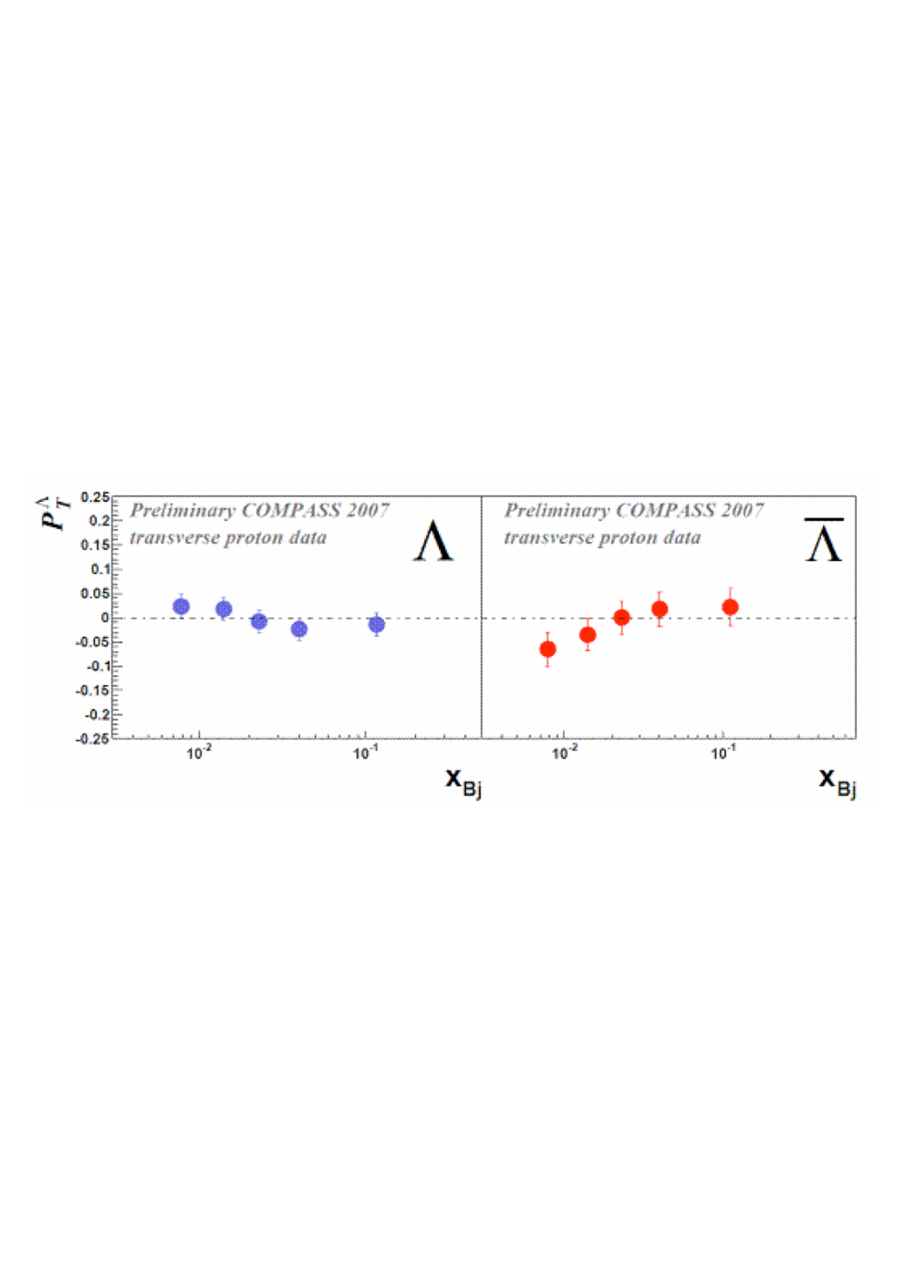
As in the case of the Collins function, independent information on can be obtained from annihilation [27, 220, 228]. The specific process is back-to-back inclusive production, , with the hyperon and the anti-hyperon decaying into and , respectively. It was shown in Ref. [220] that the unpolarised cross section of this process contains an azimuthal modulation proportional to , which is selected by the asymmetry between the number of pairs on the same side of the scattering plane and the number of pairs on opposite sides. The measurement of such asymmetry was attempted by the ALEPH Collaboration at LEP [305], but the scarce sensitivity of data did not allow getting any significant result.
5.3 Accessing TMD distributions: T-odd leading twist functions
SIDIS represents, at this moment, the best source of knowledge on the two -odd distribution functions: the Sivers function, involved in transversely polarised SIDIS, and the Boer-Mulders function, which generates asymmetries in unpolarised SIDIS. Some information on the Boer-Mulders distribution comes also from unpolarised Drell-Yan processes. DY can probe the Sivers function as well, if one of the two colliding hadrons is transversely polarised, but this reaction so far has not been experimentally explored.
5.3.1 Sivers effect in SIDIS
As in the case of the transversity PDF’s, the only measurements which give today a clean access to the Sivers function are the SSA’s in SIDIS on transversely polarised targets. The relevant quantity is the so-called Sivers asymmetry , where and are the structure functions introduced in eq.(58). This SSA couples to the unpolarised fragmentation function . Till now it has been measured only by the COMPASS and the HERMES experiments. The same data as for the measurement of the Collins asymmetry have been used, and the same kind of analysis, described in Section 5.1, has been performed. In this case the relevant modulation is that in the azimuthal angle , and, at variance with the Collins case, the Sivers asymmetry is defined in the same way and with the same sign in the COMPASS and in the HERMES experiments. It has to be noted that in the HERMES papers the Sivers asymmetry is indicated as .
The first results on the Sivers asymmetry have been produced by the HERMES experiment using the data collected in 2002 with the transversely polarised proton target [41], and showed large positive values for the and while for and the asymmetries were compatible with zero. The preliminary results from the 2002-2005 data [275] and the final results published recently [276] confirmed with better statistical precision the previous measurement.


Fig. 31 shows the final Sivers asymmetries versus , and for pions and charged kaons. The error bars are statistical only. The systematic uncertainty is shown by the bands and include possible contributions due to the longitudinal component of the target spin as well as acceptance and smearing effects, radiative effects, and effects due to the hadron identification. The additional scale error due to the target polarisation uncertainty is quoted to be 7.3%. As can be seen, the asymmetry is of the order of 5% almost over all the measured range, compatible with zero for , and slightly positive for . Slightly positive signals can be seen also for , while the values for are quite large, up to 10%. The pion results can naively be explained in the framework of the quark model. With the assumptions used in eq. (127), they can be understood as due to a the -quark Sivers function of roughly twice the size of that of the quark, and of opposite sign. The results are more difficult to be explained, and further studies on the difference between and results are quoted in [276]. Also, the asymmetry in the difference of the distributions of and , which should be more related to the and quark Sivers functions in the valence region, has been measured. Finally, a study of the dependence has been performed, without finding clear effects indicating sizable effects. It has to be reminded, however, that the mean values of are all in the range between 1 GeV2 and about 7 GeV2.
As in the Collins case, COMPASS has measured for the first time the Sivers asymmetry on the deuteron. First results for charged hadrons from the 2002 data were published in 2005 [42], and later on final results from all the collected deuteron data have been produced for charged hadrons [43] and for identified pions and kaons [280]. The measured Sivers asymmetries for identified hadrons are shown in Fig. 32.

The errors are statistical only. The quoted systematic errors are negligible with respect to the statistical ones. All the measured values are compatible with zero within the small statistical errors. This result for pions can be interpreted naively in the framework of the parton model [43] as due to opposite Sivers functions for the and quarks.
After the first phenomenological study [108] of preliminary HERMES data on the –weighted Sivers asymmetry [306], various theoretical groups [291, 287, 307, 308] extracted the Sivers distributions (or their moments) from the HERMES measurement of [41]. The fits were then extended [291, 308] to higher-precision HERMES preliminary data [309] and to the COMPASS deuteron data [42]. A comparison of the results of these analyses [310] shows a certain qualitative agreement and some common features: a negative and a positive , as predicted by the the impact-parameter approach [141], with comparable magnitudes, as expected in the large- limit [160] or in chiral models [161].
More recent fits [110, 111] take into account the new HERMES [276] and COMPASS deuteron data [280]. The surprisingly large values of the asymmetry and of the difference call for a careful reconsideration of the sea. The Sivers functions are factorised in and , with a Gaussian dependence on . Taking as an example the parametrisation of Ref. [110], the functional form of is
| (137) |
where and are free parameters, the last two being taken to be the same for all flavors. It turns out that the exponent governing the high- tail of the distributions is not well constrained by the data which extend up to . The overall quality of the fit is rather good and the first moments of the extracted Sivers functions for the and quarks displayed in Fig. 33.

As expected, a non negligible strange sea is required to reproduce the data. The and distributions are more uncertain, even in their sign.
The two fits of Ref. [110] and Ref. [111] indicate that the Burkardt sum rule is approximately saturated by the quark and antiquark distributions, thus little room is left for the gluon Sivers component and the orbital motion is restricted to valence quarks.
In this situation, in which all the existing experimental data on the Sivers asymmetry could be explained coherently, the COMPASS measurements with the transversely polarised proton target came as a surprise. The preliminary results for charged hadrons from part of the 2007 data were released in 2008 [294] and showed small asymmetries both for positive and negative hadrons, compatible with zero within the statistical errors. The analysis of the complete set of data was concluded only recently [279], and the final results are shown in Fig. 34.

For positive hadrons the data indicate small positive values, up to about 3% in the valence region. These values are somewhat smaller than but still compatible with the ones measured by HERMES at smaller . The systematic errors is estimated to be 0.8, plus a systematic uncertainty in the absolute scale due to a systematic difference in the mean values of the asymmetry which was found between the first and the second parts of the 2007 run.
Given the importance of the Sivers function the COMPASS Collaboration has decided to remeasure SSA’s on NH3 in 2010 with an improved spectrometer and better statistics.
5.3.2 Boer Mulders effect in SIDIS
The existence of and asymmetries in unpolarised SIDIS is experimentally well established. They have been investigated many years ago by the EMC and ZEUS experiments [311, 312, 313] in the large region where they are dominated by perturbative QCD effects. It is indeed known that these asymmetries are perturbatively generated by gluon radiation [193, 194, 314, 195, 315, 316] and at high and high they are dominated by these effects. The recent HERMES [317], COMPASS [318] and CLAS [319] results cover a kinematical region (small and GeV) where gluon emission is negligible [320] and the asymmetries can be described in terms of TMD’s and higher-twist contributions.
The unpolarised azimuthal asymmetries have been measured by the COMPASS and HERMES Collaborations using part of the data collected with polarised targets and combining them in order to cancel the net target polarisation.
The COMPASS preliminary results [318] have been obtained from part of the data collected in 2004 with the 6LiD target polarised both transversely and longitudinally with respect to the muon beam direction. The data have been combining in such a way to cancel the net target polarisation. To reduce the acceptance effects, only the events with a vertex in the downstream target cell have been used, and the statistics for each polarisation orientation chosen in such a way to have a zero net polarisation. The events are selected requiring the usual cuts GeV2, mass of the final hadronic state GeV, . For the final state hadrons it is required that and GeV. The data have been binned alternatively in , and and in each bin the measured distribution has been corrected for the acceptance of the spectrometer, evaluated with a Monte Carlo simulation. Since the COMPASS beam is longitudinally polarised, a modulation is also possible, so the corrected distributions have been fitted with a function containing the , the and the modulations. This last amplitude turned out to be always compatible with zero. The preliminary results for the asymmetries are shown in Fig. 35 as functions of , and for positive and negative hadrons. The measured asymmetries have been corrected for the corresponding dependent kinematical factor appearing in the cross-section.

The errors are statistical only. The systematic errors are of the order of 2% in both cases and are largely dominated by the acceptance correction. Both the and the asymmetries are quite large, with a strong dependence on the kinematical variables. Also, for the first time, the asymmetries have been produced separately for positive and negative hadrons and the measured difference points to different contributions of the and quarks to the underlying mechanisms.
The HERMES experiment has produced results for the and the asymmetries in hydrogen and deuterium using the data collected in 2000, 2005, and 2006. The cuts applied in the event and hadron selection are: , GeV2, GeV2, , , , and GeV. To correct for acceptance of the spectrometer, detector smearing, and QED radiative effects, the data were analysed in a 5-dimensional grid in the variables , , , and . A 10-dimensional smearing matrix was populated by Monte Carlo simulation and incorporated into the fitting procedure, which has been extensively tested with Monte Carlo data. The released asymmetries are one dimensional projections of the asymmetries in which the other four variables have been integrated over. The measured asymmetries for protons and deuterons are shown in Fig. 36 for positive and negative hadrons versus , , , and .


The error bars are statistical, and the bands show the systematic error. As can be seen in the figure, the proton and the deuteron asymmetries are very similar, giving a hint for alike sign for the and Boer Mulders functions. The difference between positive and negative hadrons is remarkable, as in the case of the COMPASS results. At variance with the COMPASS data shown here, the HERMES results incorporate the -dependent kinematical factor appearing in the cross section.
The CLAS results at JLab for the asymmetry for [319] agree with the HERMES measurements at large . A striking feature of their data is the large values measured for , which increase with and for which there is no comparison with other experiments.
Phenomenologically, the Cahn contribution to the asymmetry was studied by Anselmino and coworkers [291]. Using the EMC data [311, 312] in the region GeV, they extracted the average values of quark momenta: GeV2 in the distribution functions, GeV2 in the fragmentation functions.
The asymmetry has been analysed in detail in Refs.[320, 145, 321]. In Ref. [320], which anticipated the measurements, it was predicted that is of the order of at most , and that the asymmetry should be larger than the asymmetry, as a consequence of the Boer-Mulders effect. These predictions have been substantially confirmed by the experimental results. A fit to the HERMES and COMPASS preliminary data has been recently presented in Ref. [145]. It assumes that can be described by the leading-twist Boer-Mulders component and by the twist-4 Cahn term (which is however only part of the full twist-4 contribution, still unknown). The available data do not allow a complete determination of the and dependence of . Thus, the Boer-Mulders functions are simply taken to be proportional to the Sivers functions of Ref. [110], , and the parameters are obtained from the fit (the Boer-Mulders sea is not constrained by the data and is taken to be equal in magnitude to the Sivers sea). The result is
| (138) |
and the comparison with the data is shown in Fig. 37


Since is negative and is positive, the and Boer-Mulders distributions are both negative. This is what one expects in large- QCD [160] and in some other models [152, 157]. The results are also consistent with the predictions of the impact-parameter picture [87] combined with lattice calculations [143], which indicate a component of larger in magnitude than the corresponding Sivers component, and the distributions with the same magnitude and opposite sign. A very recent model calculation of [322] is in good agreement with the findings of Ref. [145].
5.3.3 Boer-Mulders effect in DY production
As shown is Section 4.3.1 the cross-section for the DY process on unpolarised nucleon is given by eq. 99 where the quantities and are related by the Lam-Tung relation .
The NA10 data on DY off a tungsten target show that the angular distribution for the DY events do not show any c.m. energy dependence nor any nuclear dependence. The data show that the value for is close to 1, as expected by the naive parton model (for massless quarks and no intrinsic quark momentum the angular distribution should just be (). Also, the value for is close to expectation: it is essentially consistent with zero, indicating that the annihilating partons contribute equally to the transverse momentum of the muon-pair. Both the values of and of are essentially independent of any kinematical variable. But the most striking result from this experiment is the large value they obtain for and the strong dependence of on the dimuon transverse momentum.
Similar results have been obtained at FermiLab by the experiment E615 which investigated the same DY process. As shown in Fig. 38 was found to be as large as 30%, and steeply rising with , an effect which is not explained by pQCD and was interpreted as a manifestation of the Boer-Mulders mechanism [240]. Also, by projecting the data points on the axis, the pion valence structure function could be precisely determined in the range from 0.21 to 1, and found in good agreement with the extraction of NA3 and NA10.

Recently, the E866/NuSea Collaboration at FNAL has presented data on the angular distributions of dimuon production in [324] and [70] collisions. Much smaller values (less than 0.05) than in DY are found, as shown in Fig. 39, and the Lam-Tung relation is satisfied. These data could in principle give some information about the antiquark Boer-Mulders distributions [325, 326]. However, in the region above 1-1.5 GeV they are expected to be described by pQCD [238]. Thus the only points that have likely to do with the Boer-Mulders effect are those below GeV.
We conclude this section by mentioning that a theoretical study of the DY azimuthal asymmetries at small and moderate in the context of twist-three factorisation has been performed in Ref. [251].


5.4 Accessing the TMD distributions: leading-twist -even functions and higher-twist functions
At leading twist, besides the Collins, Sivers and Boer–Mulders terms, there are other three angular modulations in the SIDIS cross section, which probe -even TMD distributions:
- -
Unpolarised beam and longitudinally polarised target: modulation, involving .
- -
Unpolarised beam and transversely polarised target: modulation, involving .
- -
Longitudinally polarised beam and transversely polarised target: modulation, involving .
From the data collected with the deuteron target, the COMPASS experiment has produced preliminary results on these asymmetries for charged hadrons [327, 328]. All in all, it is hard to find a signal in any of these observables. It will be interesting to look at the corresponding results with the proton target.
The HERMES collaboration has measured the moment, both with a proton [329] and a deuteron target [330], finding it to be compatible with zero. Signals of a non vanishing asymmetry have been recently reported by the CLAS collaboration [331].
For the moment, all these data can only be confronted with model predictions. Focusing on , which has attracted some attention for its interesting physical content, a calculation of based on positivity bounds [121] gives limits of about for the asymmetry on a deuteron target and a slightly larger value for a proton target. The COMPASS deuteron data lie within these bounds.
The light-cone constituent quark model of Ref. [165] predicts an asymmetry smaller than 0.01, also consistent with the COMPASS findings. All the asymmetries related to -even TMD’s are calculated in Ref. [165] and found to be generally close to zero, hence compatible with the COMPASS findings.
At subleading twist, that is at order , the situation is much more involved. The SIDIS structure functions of eq. (58) have have in fact the general form:
where “l.t.” = leading twist, and “h.t” = higher twist. They contain both leading-twist and twist-three TMD distributions and fragmentation functions. Thus, the phenomenological interpretation of these observables is rather intricate. In SIDIS with unpolarised (U) and/or longitudinally (L) and transversely (T) polarised beams and targets there are 8 twist-three modulations:
COMPASS has measured all these quantities on a deuteron target [327, 318, 328] and found them all to be consistent with zero. HERMES presented results on the and modulations with a longitudinally polarised proton [329] and deuteron target [330]. While the asymmetry was found to vanish, the asymmetry showed a large signal (up to 4% for proton and 2% in deuteron), incompatible with zero for positive and neutral pions, originally interpreted in terms of large transversity PDF’s.
A remark about the definition of the target polarisation is now in order. Experimentally, the target polarisation is defined with respect to the a longitudinal (transverse) polarisation with respect to the beam axis has a transverse (longitudinal) component with respect to the virtual photon axis, which is kinematically suppressed by a factor [112]. Thus, any measured modulation with a “longitudinally” (“transversely”) polarised target is mixed with a transverse (longitudinal) modulation of the same type, suppressed by . This may be relevant in some cases. For instance, the asymmetry measured with a target longitudinally polarised with respect to the beam axis gets a twist-three contribution from , but receives also contributions from the leading-twist Collins and Sivers asymmetries, and , which are multiplied by a kinematical factor . In principle, all these contributions might be equally relevant. The HERMES analysis of the asymmetry [332] has shown that the Collins and Sivers contributions to are small, and therefore the large measured asymmetry is a genuine subleading-twist effect.
Another indication of the relevance of twist-three effects comes from the beam-spin asymmetry , which has been measured by CLAS at 4.3 GeV for positive pions [333] and by HERMES at 27.6 GeV for charged and neutral pions [334]. The asymmetry for positive pions is large and positive. The CLAS and HERMES results nicely agree if one rescales the HERMES data by the mean value of and the dependent kinematical factor, as shown in Fig. 40.

.
5.5 Inclusive hadroproduction
Sizable SSA’s in polarised inclusive hadroproduction have been reported since the 70s [1, 2, 3, 335], for center-of mass energies in the range 5-10 GeV. In the same years, Fermilab experiments discovered that hyperons produced in unpolarised collisions have a large transverse polarisation with respect to the production plane [4, 5]. These findings provoked a certain theoretical interest, as it was widely held that large transverse polarisation effects could not be reproduced in the framework of perturbative QCD [16]. On the other hand, the small values of and explored by those experiments left the door open to interpretations based on soft physics.
In 1991 the E581/E704 experiment at Fermilab extended the investigation of transversely polarised hadroproduction to higher energies and found remarkably large transverse SSA’s in the forward region [8, 9]. These results were confirmed by the RHIC measurements, which moved the energy frontier one order of magnitude upwards. On the polarisation front, the striking effect discovered in the early experiments was observed also at higher values [336, 337, 338]. Thus, it has become clear that there must be some hard mechanism behind the transverse polarisation phenomena observed in hadroproduction.
5.5.1 SSA’s in inclusive hadroproduction
As seen in Section 5.1, the left-right asymmetries associated to an azimuthal modulation of a cross-section, are best measured by comparing data taken with up- and down-polarised beam or target. Integrating over , a global left-right asymmetry can then be defined as
| (139) |
with the beam or target polarisation.
The modern era of experimental (and theoretical) work on SSA’s in hadroproduction was inaugurated by the E704 investigation of and collisions with transversely polarised secondary proton and antiproton beams at the c.m. energy GeV [8, 9]. Two kinematical regions were covered: 1) the beam fragmentation (or forward) region, , with in the range GeV; 2) the central rapidity region, , with up to 4 GeV. In pion production, large SSA’s were found at high [8, 7, 9, 10]: the asymmetries are nearly zero up to and then start rising with , reaching 15 % for and 30-40 % for . In collisions is positive for and negative for , with about the same size. Signs are reversed in scattering. The asymmetry for is roughly half of that of charged pions and always positive. As for the dependence, is zero below GeV, and above this value increases in magnitude with . In the central rapidity region, where larger values of are reached, the asymmetries turn out to be consistent with zero [339]. E704 has also measured sizable SSA’s in inclusive and production [340, 341] but the rather low transverse momentum of the ’s does not allow a safe perturbative QCD analysis.
The E704 findings have been substantially confirmed by other fixed-target experiments at lower energies, at IHEP (Protvino) [342, 343] and at the BNL–AGS [344, 345].
On the phenomenological side,the E704 pion asymmetries have been interpreted in terms of the Sivers effect [346, 39, 257] and of the Collins effect [176, 40, 347]. A recent reassessment of the situation [348] has shown that, contrary to a previous prediction of a strong suppression of the Collins effect [349], both Collins and Sivers mechanisms may give sizable contributions to the SSA’s. The E704 results have also been studied in the context of twist-3 factorisation, considering quark-gluon correlations in the initial state [53, 55, 263, 264, 350] and in the final state [265]. All these approaches are able to reproduce at least qualitatively the data, thus showing that many different physical mechanisms may be at work in polarised hadroproduction. Thus, it is impossible for the moment to draw definite conclusions as to the dynamical source of single-spin transverse asymmetries.
The E704 measurement might have left the doubt that transverse SSA’s would disappear at collider energies. Studying the reaction at GeV in the first polarised collisions at RHIC, the STAR Collaboration showed that this is not the case: the large effects found by E704 persist at an order of magnitude higher energy [11]. As shown in Fig. 41 STAR measured a large positive above in the transverse-momentum range GeV. More recently, the negative region has been explored, finding an asymmetry consistent with zero, and the dependence of the SSA has been determined [351]. In Fig. 42 one sees that the rise of the SSA’s at large is fairly well reproduced by the Sivers mechanism in the generalised parton model with the Sivers function extracted from the HERMES SIDIS data [257, 352] and by the twist-3 factorisation scheme [350]. On the contrary the behaviour of the data, showing a clear tendency to increase at fixed , contradicts the theoretical expectations, which predict a decrease of with .
Concerning the description of hadroproduction SSA’s in terms of TMD’s taken from SIDIS analysis, one should recall that RHIC asymmetries scan the parton distributions over a wide range of the Bjorken variable, including the large- region, whereas the SIDIS data are limited to and do not constrain the tails of the transversity distribution and of the Sivers function. Thus, the generalised parton model predictions of the SSA’s are quite uncertain at high [353].


Measurements of forward charged pions by BRAHMS at GeV [354] and GeV [355] shown in Fig. 43 confirm the asymmetry pattern observed by E704, with the mirror effect of and and large absolute values of . The SSA’s for and at GeV are plotted in bins of in Fig. 44. A clear rise with is visible up to a transverse momentum of about 1 GeV, where the asymmetries reach magnitudes of about 0.3.


BRAHMS has also measured kaon production at finding that the asymmetry has the same sign and approximately the same magnitude as the asymmetry [355]. The results are fairly well reproduced both by the twist-3 approach and by the Sivers effect in the generalised parton model
In the midrapidity region (). the PHENIX measurements of neutral pion and charged hadron production at GeV [14] at GeV, showed transverse SSA’s consistent with zero. This result is in agreement with the fixed-target E704 finding and extends it to higher , up to 5 GeV.
5.5.2 Spin-averaged hadroproduction cross sections
The QCD-based descriptions of the E704 and RHIC results on hadroproduction SSA’s have been criticised [356] on the ground that, whereas the spin-averaged cross sections at GeV [12, 357, 15] are well described by next-to-leading order perturbative QCD [358], the cross sections at lower energies (for instance at GeV [339]) are not. The conclusion of Ref. [356] is that the single-spin asymmetries discovered by E704 and those found at RHIC are different physical phenomena. However, it has been recently shown that the resummation of large logarithms arising from soft gluon radiation in the limit significantly improves the agreement of perturbative QCD calculations (limited however to the cross sections integrated over rapidity) with data at low and intermediate energies [359, 360]. Predictions for GSI-FAIR and J-PARC kinematics are given in Ref. [361]. The inclusion of intrinsic transverse momentum effects has been also shown to reduce the discrepancy between QCD-parton model predictions and cross section data in the fixed-target regime [257].
Thus, the hope to achieve a consistent QCD picture of both polarised and spin-averaged hadroproduction phenomena seems to be well founded.
6 Future measurements
In this section account is given of near future and more distant future SIDIS and DY experiments. The main goal of the SIDIS experiments is to measure the SSA’s over a detailed grid of the kinematic variables , , and , facilitating the extraction of the DF’s and of the FF’s. In addition, it should be possible to study sub-leading twist effects by probing their dependence, and to explore the transition from non-perturbative small transverse momentum, typically lower than 1 GeV, to the transverse momentum large regime. In the case of the DY measurements, the main goal is to perform for the first time experiments with polarised nucleon targets and/or polarised beams, to test the predicted test of sign of the T-odd DF’s.
6.1 SIDIS experiments
COMPASS at CERN:
The analysis of the 2007 transversely polarised proton data is still ongoing,
and several results on SSA’s have still to be obtained.
Many more data on the
same target (NH3) will be collected in the long 2010 run, so that in
the near future a large amount of data is expected.
For what concerns a more distant future,
the COMPASS Collaboration is presently preparing a proposal for
measurements aiming to study chiral perturbation theory,
generalised parton distributions via Deeply Virtual Compton Scattering
(DVCS), and TMD parton distributions via Drell-Yan processes.
The DVCS measurements will be performed using a liquid hydrogen target
and a 190 GeV muon beam.
In parallel with these measurements, SIDIS data will be collected
to extract with high precision the unpolarised and
azimuthal asymmetries as well as the beam helicity dependent
asymmetry.
Such information cannot be extracted from the data collected
with the transversely polarised target because of the complications
of using a nuclear target.
JLab experiments:
In the near future also the CLAS Collaboration in Hall B will take SIDIS data
on a transversely polarised target. For transverse running, the use
of a novel HD-ice target is planned, which in a frozen-spin state requires
only small holding fields.
The use of the HD-ice
target by the E08-015 Collaboration has many advantages: being a solid
target, it can be short, a few cm, and thanks to the smallness of the holding
field it can be located in the centre of the detector, thus increasing the
acceptance of the spectrometer. In addition, the HD target has almost no
dilution, which maximises the figure-of-merit, and being of low atomic number,
comparatively few bremsstrahlung photons will be produced in the target. The
experiment should run in the second half of 2011, and an upgraded version of
the detector has already been proposed for JLab12.
In a medium term range,
Jlab12 GeV upgrade could meet the requirements to study TMD’s in the
valence region, thus covering a complementary kinematic region with respect
to COMPASS.
The Clas12 experiment in Hall-B is designed to achieve a very broad
kinematic coverage while increasing by a factor 10 the luminosity with
respect to the current 6 GeV setup.
In particular, the forward spectrometer comprises a 2 T toroid with
improved geometry to minimise the not-active azimuthal coverage and
a RICH detector is under study to extend the hadron identification over
the full energy range of the experiment.
The spectrometer
is complemented by a central detector embedded in a 5 T solenoid.
Also, an upgraded version of experiment E06-010 (PR09-018) has already
been proposed and conditionally approved to run in Hall A.
The experiment aims to measure the SSA’s of the SIDIS process
, where is either a or a .
The experiment will use the large-solid-angle Super BigBite Spectrometer
as hadron arm, the BigBite Spectrometer as electron arm, and a novel
polarised 3He target that includes alkali-hybrid optical pumping
and convection flow to achieve very high luminosity.
Thanks to the large acceptances of the electron and hadron arms,
an electron - polarised nucleon luminosity at the level of
cm-2s-1, and a target polarisation of 65%,
the experiment should collect in a two-month run about 100 times more
statistics than that obtained by the past experiments.
and future colliders:
In depth studies of hadron structure can be best performed at a high energy
polarised electron-polarised proton collider.
Large Collaborations at BNL and JLab are
elaborating proposals which are well advanced and are being encouraged
by the USA agencies. As written in the NSAC 2007 Long Range Plan,
”the allocation of resources are recommended to develop accelerator
and detector technology necessary to lay the foundation for a polarised
Electron Ion Collider (EIC).
The EIC would explore the new QCD frontier of strong color
fields in nuclei and precisely image the gluons in the proton”.
To carry out a rich and diversified physics program the
recommended energies for the electrons are between 3 and 10 GeV,
for the protons between 25 and 250 GeV, and for the heavy ions
between 25 and 100 GeV.
The luminosity in the case of the collider should be
cm-2s-1, i.e. about 100 times the luminosity of the HERA collider.
Recently preliminary ideas for a polarised electron-nucleon collider
(ENC) at GSI, Darmstadt, have been discussed mostly amongst the German
community.
The advantage of the Collider configuration over fixed target experiments
are manifold:
- it provides a large range of , , and .
- the figure of merit for asymmetry measurements is
very much better.
For ammonia (NH3) , thus the figure of merit when
scattering on a pure proton beam is better by a factor .
Needless to say, the comparison is done assuming the same number of
collected events, so a high luminosity for the EIC is a prerequisite.
- It provides access to the interaction region, so that modern vertex
tracking systems can identify short living particles, like produced
in the interaction.
Having access to the interaction region, exclusive reactions are at reach.
This opens up the whole field of GPDs, which to-day are the only way to
quantify how the orbital motion of quarks in the nucleon contributes to
the nucleon spin.
Also, it allows measurements in the
target fragmentation region, which is presently poorly known due to
the difficulty of measuring slowly moving hadrons in fixed-target
experiments, opening a window to
the study of spin-independent and spin-dependent ”fracture” functions.
The US groups of RHIC and JLab are proceeding jointly to the formulation of
two different proposals for two different colliders, eRHIC and ELIC, based
in the two different laboratories.
The RHIC project clearly foresees the use of the highly polarised proton
and nuclear existing beams.
Two accelerator design options are being worked upon, both aiming at high
brightness 10 GeV electron beams.
A Ring-Ring option, which requires a new electron storage ring for
polarised electron or positron beams, is technologically more mature,
and could provide a peak luminosity of cm-2s-1.
The second option is a Linac-Ring option, which offers higher
luminosity (by a factor of 5) and possibly higher energy,
but requires intensive R&D for the high-current polarised electron source.
The starting point of the JLab project is the availability of the
12 GeV electron beam from the upgraded CEBAF.
The proton complex has to be built from scratch, so it
is being designed taking full advantage of the
expertise matured at RHIC and other laboratories on acceleration and
storage of polarised proton beams.
The design goal for the collider luminosity is very ambitious,
cm-2s-1 for beam energies of 10 and
250 GeV for the electron and protons respectively.
Quite recently, in the summer of 2008, discussions
started22
2
Private communication from D. von Harrach.,
about a possible low-cost realisation of an ENC at GSI.
The central idea is to use the 15 GeV high energy storage ring HESR,
which is planned to store an antiproton beam for the PANDA experiment
(and possibly PAX) as the ring where to store the polarised proton beam.
By constructing a 3-3.5 GeV electron ring, a ”low energy” ENC could be
realised. The cm energy would be 14 GeV, i.e. in between the HERMES and
the COMPASS energies.
To inject polarised protons in HESR a new 70 MeV -linac will be needed.
The protons would then be injected into the existing SIS18 ring, accelerated
up to 1.4 GeV, and transferred then into HESR. New hardware for the spin
manipulations will be needed in SIS 18 and in HESR, but it is the same
which will be necessary for the PAX experiment.
The electron complex has to be constructed from scratch. An -linac and
an electron synchrotron will accelerate the electron beam, which will
be stored into a new storage ring of about the same length as HESR,
and housed in the same tunnel.
Preliminary machine studies indicate that a luminosity of at least
could be achieved, as well as large polarisations ( 80%) for the two beams.
To further reduce the cost of the project, it is proposed to use the PANDA
detector, and to operate the collider in time sharing with the PANDA
Collaboration.
6.2 Drell-Yan
As described in section 4.3, the DY process in transversely polarised hadron scattering is theoretically a very clean and safe way to access transversity. The original suggestion of measuring DY in scattering, which could be done at RHIC, turned out to be difficult because of the small value expected for the asymmetry,of the order of % [83, 245, 246]. The measurement will also require external input to disentangle the quark and the antiquark distributions. It will be done when the RHIC luminosity will be increased.
These problems can be circumvented by studying DY production with polarised antiprotons at moderate energies, which is the ideal process to observe a sizable double transverse asymmetry [83, 362, 363, 247], dominated by the valence distributions. Such a measurement has been proposed by the PAX Collaboration [232] at the FAIR complex to be built at GSI. Since the production rate for relatively large dilepton masses ( GeV) might be too small to allow an easy measurement , it has been proposed [362] to exploit the peak to measure the asymmetry.
Finally, we recall that the Sivers effect can also be observed in Drell-Yan processes with a transversely polarised proton, where it gives rise to a asymmetry. No measurement has been made so far, but many experimental collaborations worldwide plan to investigate this class of reactions in the near future.
6.2.1 The proposed experiments
In the following we describe very briefly the DY proposed experiments.
COMPASS: Among the proposed measurements for a second phase of the COMPASS experiment an important issue is the possibility to investigate for the first time a induced DY process on a transversely polarised proton target. The high mass of the COMPASS target (about 1 kg of NH3) and the excellent performance of the COMPASS spectrometer make this measurement feasible, and the number of events collected in two years of running would allow to check the expected change of sign of the Sivers function. Assuming for the magnitude of the Sivers function the value extracted from the HERMES measurements in SIDIS (see Fig. 45, left), the significance of the measurement is expected to be 3 to 4 .
PAX and PANDA at GSI: As already mentioned, the PAX Collaboration has proposed to measure DY processes in scattering at FAIR. An asymmetric collider is proposed, consisting of HESR, where polarised protons will be stored, and of a new storage ring for the polarised antiprotons, which could be the existing COSY Storage Ring, suitably modified. The predictions for in collisions at GSI-FAIR are shown in Fig. 45 (right). One sees that asymmetries of the order of 10-15 % can be expected at PAX.


Polarisation of the stored antiproton beam will be done using the
“spin filtering” technique [365].
The antiprotons beam traverses a polarised proton storage cell, and a
beam polarisation builds up by repeatedly passing through the cell
as long as the cross section for parallel spin is different from that of
antiparallel spins.
The method has been proven to work for proton beams, but in the case of
antiprotons the spin dependent cross-sections are not known and corresponding
measurements have been proposed at the Antiproton Decelerator at CERN.
The PANDA collaboration also envisage the measurement of DY process in
scattering, where both particles are unpolarised.
The option to put a transversely polarised proton target in the PANDA
detector is very interesting, but it is technically very difficult and has
presently been discarded.
Fermilab Experiment E906:
This experiment is scheduled to run in 2010 for 2 years of data collection.
It will extend DY measurements of E866 (which were done with 800 GeV
protons) using an upgraded spectrometer and the 120 GeV proton beam from
the main injector.
The use of the lower beam energy gives a factor 50
improvement of luminosity with respect to E866.
To cut down costs, it will use many components from E866, and data will
be taken with Hydrogen, Deuterium and Nuclear Targets.
The main goal of the experiment is the study of the structure of the
nucleon, in particular the ratio at high .
In the future, there are plans to measure SSA’s on a transversely
polarised target,
and check the change of sign of the Sivers function with respect to SIDIS.
J–PARC:
Two proposals for DY experiments have been submitted:
- P04: measurement of high-mass dimuon production at the 50 GeV
proton synchrotron;
- P24: polarised proton acceleration.
The advantage of an experiment at JAPRC is the high proton beam intensity, and
consequently the high luminosity.
The disadvantage is that at the same invariant
mass the cross section is smaller at lower energy.
The transverse polarisation
program is best carried on by P24, but is clearly conditioned by the
realisation of the polarised proton beam, which is not yet approved.
STAR and PHENIX at RHIC: According to the present accelerator schedule, which foresees a long longitudinal run for W-physics, a DY program with transverse spin at PHENIX and STAR will not start before 2015. However, since in the intersection regions IP-2 and IP-10, where the PHOBOS and the BRAHMS experiments were installed, there are no spin rotators, the polarisation of the beams is always transverse and ideas are being put forward to prepare both a collider experiment and a fixed target experiment for DY measurements.
RHIC internal target: Quite recently ideas have been put forward for a DY experiment at RHIC scattering one beam off an internal target. With the 250 GeV beam, the kinematic range explored would be (), which would be ideal to investigate the change of sign of the Sivers function. To achieve the necessary luminosity, the use of a pellet target is being investigated, in two different scenarios according to the target thickness (parasitic running or dedicated experiment).
NICA: To investigate the hadron structure a Nuclotron-based Ion Collider fAcility (NICA) is being planned at the JINR in Dubna, based on the existing proton synchrotron Nuclotron. The accelerator complex will require new ion and polarised proton sources, a new linear accelerator, a new booster synchrotron and the two new superconducting storage rings of the collider. Both polarised proton and polarised deuteron beams should be available in the two rings. The main physics objectives will be the study of elastic processes and of Drell-Yan processes.
6.2.2 Summary
The relevant parameters for all these projects are summarised in Table 1.
| Experiment | particles | energy | or | luminosity | |
|---|---|---|---|---|---|
| COMPASS | 160 GeV | 17.4 GeV | cm-2s-1 | ||
| PAX | collider | 14 GeV | cm-2s-1 | ||
| PANDA | 15 GeV | 5.5 GeV | cm-2s-1 | ||
| J–PARC | 50 GeV | 10 GeV | cm-2s-1 | ||
| NICA | collider | 20 GeV | cm-2s-1 | ||
| RHIC | collider | 500 GeV | cm-2s-1 | ||
| RHIC IT phase 1 | 250 GeV | 22 GeV | cm-2s-1 | ||
| RHIC IT phase 2 | 250 GeV | 22 GeV | cm-2s-1 |
Theoretical predictions for COMPASS (), PAX (), RHIC ( at GeV) and J–PARC ( at GeV) have been presented by various authors [108, 366, 367, 368, 369, 370, 364, 371, 372]. The conclusion one can draw from these analyses is that the future experiments will largely be complementary to each other.
As for DY, the RHIC data in the negative region will probe the contribution of the sea Sivers function, while experiments at lower energies, like J–PARC (operating at GeV) will provide information on the large- behaviour of . A comprehensive discussion of all future DY measurements of Sivers asymmetries can be found in Ref. [364].
7 Conclusions and perspectives
The original finding of the EMC collaboration, that the quark spin does not account for the total spin of the proton, has been a strong motivation for in-depth studies of the QCD structure of the nucleon and for a new generation of experimental investigation of hard scattering processes on polarised nucleons. The growing interest in the contribution of the quark and gluon orbital angular momentum to the nucleon spin naturally led to an increased attention to transverse spin and transverse momentum phenomena.
In this context, the most important experimental finding has been the discovery that there is a correlation between the spin of a transversely polarised quarks and the of the hadrons created in the quark hadronisation process. Convincing evidence for this correlation has been provided by both SIDIS processes on transversely polarised nucleons and high energy annihilations into hadrons. Thanks to this correlation, it is now possible to measure the transversity distribution function. Global analysis of the existing SIDIS data and of the data have already provided first rough information of this two new function.
A second important discovery of the recent years is that there is also a non-zero correlation between the spin of a transversely polarised nucleon and the intrinsic transverse momentum of the quarks.
In polarised proton-proton scattering the most impressive result in transverse spin physics is the confirmation that large SSA’s for inclusive mesons production persist at centre of mass energies which by now are more than one order of magnitude greater than those of the previous fixed target experiments.
On the theoretical side, the main achievement has been the discovery that the Wilson line structure of parton distributions, which is necessary to enforce gauge invariance, has also striking observable consequences, allowing for single-spin asymmetries that would otherwise be forbidden by time-reversal symmetry. At leading order the most general descriptions of SIDIS and Drell-Yan processes have been revisited and a number of structure functions have been introduced to take into account all possible correlations among the transverse momentum and spin of the quarks and the spin of the nucleon. Many QCD studies have been performed to understand the properties and the gauge structure of these unintegrated distribution functions, which have been named transverse momentum dependent distribution functions. Non-collinear factorisation schemes have been developed and extended to polarised processes. In an alternative approach, twist-three effects have been evaluated and compared to the TMD description in the intermediate region. A third line of attack which is vigorously being pursued is QCD computation on the lattice. Recent refined lattice QCD results shed light on the fine structure of TMD’s. This approach is particularly interesting for transversity, because the tensor charge, the first moment of the transversity distribution, which is an all-valence object, is believed to have been evaluated with good accuracy on the lattice, thus a good measurement of this quantity could provide a good test of the correctness of the calculation.
In spite of these achievements, the amount of work which is still needed is not small.
On the experimental side, the available SIDIS data are only a glimpse to a new territory, and many more data are needed to obtain the and dependence of the asymmetries in the different x-bins, a prerequisite to a model independent extraction of the TMD functions. The situation is worse however in the DY sector, since no polarised DY data exist at all. The existing unpolarised DY data allow only to access the Boer-Mulders function, but the full exploitation of the DY potential is not even at the horizon.
On the theoretical side, the present fits to the data do not make use of the evolution schemes which are already now available for the TMD’s and for the quark-gluon correlators, and which clearly must be integrated in the calculations. Also , a better understanding of higher-twist contributions to SIDIS observables (which are significant since is rather small) requires more insight and more effort.
In the near future more data will be collected in the SIDIS sector by the COMPASS and by the JLab experiments at quite different energies. In the proton-proton sector, the luminosity of the RHIC collider should be enough to allow for measurements of DY processes.
In a more distant future, COMPASS should providing new measurements of azimuthal asymmetries in SIDIS on a liquid hydrogen target and a the first measurement of polarised DY process in scattering. Also, higher energy SIDIS data will come from JLab upgraded at 12 GeV.
In an even more distant future, many projects have been proposed. The PAX experiment at FAIR aims to investigate DY pairs in polarised antiproton-polarised proton scattering, a very clean way to address the transversity functions, and a terribly difficult experiment. Fixed target DY experiments scattering polarised protons on polarised protons are being planned at JPARC, in Japan, and at NICA, in Dubna. It is fair to say, however, that the future of the field will depend in a crucial way on the pending decisions to construct a polarised electron-polarised proton collider. Ambitious projects are being pursued at BNL and at JLab. In Europe, the electron-proton collider has a long story, which needs not to be summarised here, we only mention the most recent proposal for a polarised collider, which is tailored to the new accelerators complex FAIR presently being realised at GSI. All these projects are based on existing laboratories and existing infrastructures so that optimism is mandatory.
8 Acknowledgments
This review on transverse spin and transverse momentum phenomena in hard processes has been possible thanks to the friendly exchange of ideas and information which characterizes the ”spin community”, and we would like to thank all our colleagues for their invaluable contribution in elucidating the many facets of this new and rapidly growing field. This work has been partly supported by the Italian Ministry for Education, University and Research (MIUR) as a Research Project of National Interest (PRIN).
References
- [1] L. Dick et al., Phys. Lett. B57, 93 (1975).
- [2] R. D. Klem et al., Phys. Rev. Lett. 36, 929 (1976).
- [3] W. H. Dragoset et al., Phys. Rev. D18, 3939 (1978).
- [4] G. Bunce et al., Phys. Rev. Lett. 36, 1113 (1976).
- [5] K. J. Heller et al., Phys. Rev. Lett. 41, 607 (1978).
- [6] I. P. Auer et al., FERMILAB-PROPOSAL-0581.
- [7] E581, D. L. Adams et al., Phys. Lett. B261, 201 (1991).
- [8] FNAL-E704, D. L. Adams et al., Phys. Lett. B264, 462 (1991).
- [9] E581, D. L. Adams et al., Z. Phys. C56, 181 (1992).
- [10] Fermilab E704, A. Bravar et al., Phys. Rev. Lett. 77, 2626 (1996).
- [11] STAR, J. Adams et al., Phys. Rev. Lett. 92, 171801 (2004), hep-ex/0310058.
- [12] STAR, J. Adams et al., Phys. Rev. Lett. 97, 152302 (2006), nucl-ex/0602011.
- [13] PHENIX, S. S. Adler et al., Phys. Rev. Lett. 91, 241803 (2003), hep-ex/0304038.
- [14] PHENIX, S. S. Adler et al., Phys. Rev. Lett. 95, 202001 (2005), hep-ex/0507073.
- [15] BRAHMS, I. Arsene et al., Phys. Rev. Lett. 98, 252001 (2007), hep-ex/0701041.
- [16] G. L. Kane, J. Pumplin, and W. Repko, Phys. Rev. Lett. 41, 1689 (1978).
- [17] A. V. Efremov and O. V. Teryaev, Sov. J. Nucl. Phys. 36, 140 (1982).
- [18] A. V. Efremov and O. V. Teryaev, Sov. J. Nucl. Phys. 39, 962 (1984).
- [19] P. G. Ratcliffe, Nucl. Phys. B264, 493 (1986).
- [20] V. Barone, A. Drago, and P. G. Ratcliffe, Phys. Rept. 359, 1 (2002), hep-ph/0104283.
- [21] X. Artru and M. Mekhfi, Z. Phys. C45, 669 (1990).
- [22] R. L. Jaffe and X.-D. Ji, Phys. Rev. Lett. 67, 552 (1991).
- [23] R. L. Jaffe and X.-D. Ji, Nucl. Phys. B375, 527 (1992).
- [24] J. L. Cortes, B. Pire, and J. P. Ralston, Z. Phys. C55, 409 (1992).
- [25] J. P. Ralston and D. E. Soper, Nucl. Phys. B152, 109 (1979).
- [26] N. Christ and T. D. Lee, Phys. Rev. 143, 1310 (1966).
- [27] X. Artru, (1992), hep-ph/9301296.
- [28] X. Artru, (1993), hep-ph/9310323.
- [29] J. C. Collins, Nucl. Phys. B396, 161 (1993), hep-ph/9208213.
- [30] J. C. Collins, S. F. Heppelmann, and G. A. Ladinsky, Nucl. Phys. B420, 565 (1994), hep-ph/9305309.
- [31] X.-D. Ji, Phys. Lett. B284, 137 (1992).
- [32] R. L. Jaffe, Phys. Rev. D54, 6581 (1996), hep-ph/9605456.
- [33] R. L. Jaffe, X.-m. Jin, and J. Tang, Phys. Rev. Lett. 80, 1166 (1998), hep-ph/9709322.
- [34] D. W. Sivers, Phys. Rev. D41, 83 (1990).
- [35] D. W. Sivers, Phys. Rev. D43, 261 (1991).
- [36] S. J. Brodsky, D. S. Hwang, and I. Schmidt, Phys. Lett. B530, 99 (2002), hep-ph/0201296.
- [37] S. J. Brodsky, D. S. Hwang, and I. Schmidt, Nucl. Phys. B642, 344 (2002), hep-ph/0206259.
- [38] J. C. Collins, Phys. Lett. B536, 43 (2002), hep-ph/0204004.
- [39] M. Anselmino and F. Murgia, Phys. Lett. B442, 470 (1998), hep-ph/9808426.
- [40] M. Anselmino, M. Boglione, and F. Murgia, Phys. Rev. D60, 054027 (1999), hep-ph/9901442.
- [41] HERMES, A. Airapetian et al., Phys. Rev. Lett. 94, 012002 (2005), hep-ex/0408013.
- [42] COMPASS, V. Y. Alexakhin et al., Phys. Rev. Lett. 94, 202002 (2005), hep-ex/0503002.
- [43] COMPASS, E. S. Ageev et al., Nucl. Phys. B765, 31 (2007), hep-ex/0610068.
- [44] Belle, K. Abe et al., Phys. Rev. Lett. 96, 232002 (2006), hep-ex/0507063.
- [45] M. Anselmino et al., Phys. Rev. D75, 054032 (2007), hep-ph/0701006.
- [46] A. M. Kotzinian, Nucl. Phys. B441, 234 (1995), hep-ph/9412283.
- [47] R. D. Tangerman and P. J. Mulders, Phys. Rev. D51, 3357 (1995), hep-ph/9403227.
- [48] P. J. Mulders and R. D. Tangerman, Nucl. Phys. B461, 197 (1996), hep-ph/9510301.
- [49] R. D. Tangerman and P. J. Mulders, Phys. Lett. B352, 129 (1995), hep-ph/9501202.
- [50] D. Boer and P. J. Mulders, Phys. Rev. D57, 5780 (1998), hep-ph/9711485.
- [51] X.-d. Ji, J.-p. Ma, and F. Yuan, Phys. Rev. D71, 034005 (2005), hep-ph/0404183.
- [52] X.-d. Ji, J.-P. Ma, and F. Yuan, Phys. Lett. B597, 299 (2004), hep-ph/0405085.
- [53] J.-w. Qiu and G. Sterman, Phys. Rev. Lett. 67, 2264 (1991).
- [54] J.-w. Qiu and G. Sterman, Nucl. Phys. B378, 52 (1992).
- [55] J.-w. Qiu and G. Sterman, Phys. Rev. D59, 014004 (1999), hep-ph/9806356.
- [56] X. Ji, J.-W. Qiu, W. Vogelsang, and F. Yuan, Phys. Rev. Lett. 97, 082002 (2006), hep-ph/0602239.
- [57] X. Ji, J.-w. Qiu, W. Vogelsang, and F. Yuan, Phys. Rev. D73, 094017 (2006), hep-ph/0604023.
- [58] Y. Koike, W. Vogelsang, and F. Yuan, Phys. Lett. B659, 878 (2008), arXiv:0711.0636 [hep-ph].
- [59] Z.-B. Kang and J.-W. Qiu, Phys. Rev. D79, 016003 (2009), arXiv:0811.3101 [hep-ph].
- [60] J. Zhou, F. Yuan, and Z.-T. Liang, Phys. Rev. D79, 114022 (2009), arXiv:0812.4484 [hep-ph].
- [61] V. M. Braun, A. N. Manashov, and B. Pirnay, Phys. Rev. D80, 114002 (2009), arXiv:0909.3410 [hep-ph].
- [62] W. Vogelsang and F. Yuan, Phys. Rev. D79, 094010 (2009), arXiv:0904.0410 [hep-ph].
- [63] U. D’Alesio and F. Murgia, Prog. Part. Nucl. Phys. 61, 394 (2008), arXiv:0712.4328 [hep-ph].
- [64] M. Burkardt, A. Miller, and W. D. Nowak, Rept. Prog. Phys. 73, 016201 (2010), arXiv:0812.2208 [hep-ph].
- [65] P. J. Mulders and J. Rodrigues, Phys. Rev. D63, 094021 (2001), hep-ph/0009343.
- [66] M. Diehl, Phys. Rept. 388, 41 (2003), hep-ph/0307382.
- [67] NA10, S. Falciano et al., Phys. Lett. B158, 92 (1985).
- [68] NA10, M. Guanziroli et al., Z. Phys. C37, 545 (1988).
- [69] J. S. Conway et al., Phys. Rev. D39, 92 (1989).
- [70] FNAL E866/NuSea, L. Y. Zhu et al., Phys. Rev. Lett. 102, 182001 (2009), arXiv:0811.4589 [nucl-ex].
- [71] R. P. Feynman, Photon–Hadron Interactions (Benjamin, 1972).
- [72] D. E. Soper, Phys. Rev. D15, 1141 (1977).
- [73] D. E. Soper, Phys. Rev. Lett. 43, 1847 (1979).
- [74] J. C. Collins, Acta Phys. Polon. B34, 3103 (2003), hep-ph/0304122.
- [75] R. L. Jaffe, hep-ph/9602236.
- [76] Y. L. Dokshitzer, Sov. Phys. JETP 46, 641 (1977).
- [77] V. N. Gribov and L. N. Lipatov, Sov. J. Nucl. Phys. 15, 675 (1972).
- [78] G. Altarelli and G. Parisi, Nucl. Phys. B126, 298 (1977).
- [79] A. Hayashigaki, Y. Kanazawa, and Y. Koike, Phys. Rev. D56, 7350 (1997), hep-ph/9707208.
- [80] S. Kumano and M. Miyama, Phys. Rev. D56, R2504 (1997), hep-ph/9706420.
- [81] W. Vogelsang, Phys. Rev. D57, 1886 (1998), hep-ph/9706511.
- [82] V. Barone, Phys. Lett. B409, 499 (1997), hep-ph/9703343.
- [83] V. Barone, T. Calarco, and A. Drago, Phys. Rev. D56, 527 (1997), hep-ph/9702239.
- [84] J. Soffer, Phys. Rev. Lett. 74, 1292 (1995), hep-ph/9409254.
- [85] C. Bourrely, J. Soffer, and O. V. Teryaev, Phys. Lett. B420, 375 (1998), hep-ph/9710224.
- [86] B. L. G. Bakker, E. Leader, and T. L. Trueman, Phys. Rev. D70, 114001 (2004), hep-ph/0406139.
- [87] M. Burkardt, Phys. Rev. D72, 094020 (2005), hep-ph/0505189.
- [88] M. Burkardt, Phys. Lett. B639, 462 (2006).
- [89] J. C. Collins and D. E. Soper, Nucl. Phys. B193, 381 (1981).
- [90] X.-d. Ji and F. Yuan, Phys. Lett. B543, 66 (2002), hep-ph/0206057.
- [91] A. V. Belitsky, X. Ji, and F. Yuan, Nucl. Phys. B656, 165 (2003), hep-ph/0208038.
- [92] A. Idilbi, X.-d. Ji, J.-P. Ma, and F. Yuan, Phys. Rev. D70, 074021 (2004), hep-ph/0406302.
- [93] G. A. Miller, Phys. Rev. C76, 065209 (2007), arxiv:0708.2297 [nucl-th].
- [94] H. Avakian, A. V. Efremov, P. Schweitzer, and F. Yuan, Phys. Rev. D78, 114024 (2008), arXiv:0805.3355 [hep-ph].
- [95] M. Boglione and P. J. Mulders, Phys. Rev. D60, 054007 (1999), hep-ph/9903354.
- [96] A. Bacchetta, M. Boglione, A. Henneman, and P. J. Mulders, Phys. Rev. Lett. 85, 712 (2000), hep-ph/9912490.
- [97] J. C. Collins and A. Metz, Phys. Rev. Lett. 93, 252001 (2004), hep-ph/0408249.
- [98] C. J. Bomhof, P. J. Mulders, and F. Pijlman, Phys. Lett. B596, 277 (2004), hep-ph/0406099.
- [99] A. Bacchetta, C. J. Bomhof, P. J. Mulders, and F. Pijlman, Phys. Rev. D72, 034030 (2005), hep-ph/0505268.
- [100] C. J. Bomhof, P. J. Mulders, and F. Pijlman, Eur. Phys. J. C47, 147 (2006), hep-ph/0601171.
- [101] C. J. Bomhof and P. J. Mulders, JHEP 02, 029 (2007), hep-ph/0609206.
- [102] C. J. Bomhof, P. J. Mulders, W. Vogelsang, and F. Yuan, Phys. Rev. D75, 074019 (2007), hep-ph/0701277.
- [103] C. J. Bomhof and P. J. Mulders, Nucl. Phys. B795, 409 (2008), arXiv:0709.1390 [hep-ph].
- [104] T. C. Rogers and P. J. Mulders, Phys. Rev. D81, 094006 (2010), arXiv:1001.2977 [hep-ph].
- [105] STAR, B. I. Abelev et al., Phys. Rev. Lett. 99, 142003 (2007), arXiv:0705.4629 [hep-ex].
- [106] M. Burkardt, Phys. Rev. D69, 057501 (2004), hep-ph/0311013.
- [107] M. Burkardt, Phys. Rev. D69, 091501 (2004), hep-ph/0402014.
- [108] A. V. Efremov, K. Goeke, S. Menzel, A. Metz, and P. Schweitzer, Phys. Lett. B612, 233 (2005), hep-ph/0412353.
- [109] K. Goeke, S. Meissner, A. Metz, and M. Schlegel, Phys. Lett. B637, 241 (2006), hep-ph/0601133.
- [110] M. Anselmino et al., Eur. Phys. J. A39, 89 (2009), arXiv:0805.2677 [hep-ph].
- [111] S. Arnold, A. V. Efremov, K. Goeke, M. Schlegel, and P. Schweitzer, (2008), arXiv:0805.2137 [hep-ph].
- [112] V. Barone and P. G. Ratcliffe, Transverse spin physics (World Scientific, Singapore, 2003).
- [113] R. K. Ellis, W. Furmanski, and R. Petronzio, Nucl. Phys. B207, 1 (1982).
- [114] R. K. Ellis, W. Furmanski, and R. Petronzio, Nucl. Phys. B212, 29 (1983).
- [115] J. Zhou, F. Yuan, and Z.-T. Liang, (2009), arXiv;0909.2238 [hep-ph].
- [116] D. Boer, P. J. Mulders, and F. Pijlman, Nucl. Phys. B667, 201 (2003), hep-ph/0303034.
- [117] S. Wandzura and F. Wilczek, Phys. Lett. B72, 195 (1977).
- [118] M. Anselmino, A. Efremov, and E. Leader, Phys. Rept. 261, 1 (1995), hep-ph/9501369.
- [119] A. Accardi, A. Bacchetta, W. Melnitchouk, and M. Schlegel, JHEP 11, 093 (2009), arXiv:0907.2942 [hep-ph].
- [120] R. D. Tangerman and P. J. Mulders, (1994), hep-ph/9408305.
- [121] H. Avakian et al., Phys. Rev. D77, 014023 (2008), arXiv:0709.3253 [hep-ph].
- [122] A. Metz, P. Schweitzer, and T. Teckentrup, Phys. Lett. B680, 141 (2009), arXiv:0810.5212 [hep-ph].
- [123] A. Kotzinian, B. Parsamyan, and A. Prokudin, Phys. Rev. D73, 114017 (2006), hep-ph/0603194.
- [124] A. Bacchetta, P. J. Mulders, and F. Pijlman, Phys. Lett. B595, 309 (2004), hep-ph/0405154.
- [125] K. Goeke, A. Metz, and M. Schlegel, Phys. Lett. B618, 90 (2005), hep-ph/0504130.
- [126] A. Bacchetta et al., JHEP 02, 093 (2007), hep-ph/0611265.
- [127] P. Hoodbhoy and X.-D. Ji, Phys. Rev. D50, 4429 (1994), hep-ph/9307304.
- [128] R. Kundu and A. Metz, Phys. Rev. D65, 014009 (2002), hep-ph/0107073.
- [129] K. Goeke, A. Metz, P. V. Pobylitsa, and M. V. Polyakov, Phys. Lett. B567, 27 (2003), hep-ph/0302028.
- [130] A. V. Radyushkin, Phys. Lett. B380, 417 (1996), hep-ph/9604317.
- [131] X.-D. Ji, Phys. Rev. Lett. 78, 610 (1997), hep-ph/9603249.
- [132] K. Goeke, M. V. Polyakov, and M. Vanderhaeghen, Prog. Part. Nucl. Phys. 47, 401 (2001), hep-ph/0106012.
- [133] A. V. Belitsky and A. V. Radyushkin, Phys. Rept. 418, 1 (2005), hep-ph/0504030.
- [134] S. Boffi and B. Pasquini, Riv. Nuovo Cim. 30, 387 (2007), arXiv:0711.2625 [hep-ph].
- [135] S. Meissner, A. Metz, and K. Goeke, Phys. Rev. D76, 034002 (2007), hep-ph/0703176.
- [136] M. Diehl, Eur. Phys. J. C19, 485 (2001), hep-ph/0101335.
- [137] S. Meissner, A. Metz, and M. Schlegel, (2008), arXiv:0807.1154 [hep-ph].
- [138] M. Burkardt, Int. J. Mod. Phys. A18, 173 (2003), hep-ph/0207047.
- [139] M. Diehl and P. Hagler, Eur. Phys. J. C44, 87 (2005), hep-ph/0504175.
- [140] M. Burkardt and D. S. Hwang, Phys. Rev. D69, 074032 (2004), hep-ph/0309072.
- [141] M. Burkardt, Phys. Rev. D66, 114005 (2002), hep-ph/0209179.
- [142] M. Burkardt, Nucl. Phys. A735, 185 (2004), hep-ph/0302144.
- [143] QCDSF, M. Göckeler et al., Phys. Rev. Lett. 98, 222001 (2007), hep-lat/0612032.
- [144] QCDSF-UKQCD, D. Brömmel et al., Prog. Part. Nucl. Phys. 61, 73 (2008).
- [145] V. Barone, S. Melis, and A. Prokudin, Phys. Rev. D81, 114026 (2010), arXiv:0912.5194 [hep-ph].
- [146] H. Avakian et al., Mod. Phys. Lett. A24, 2995 (2009), arXiv:0910.3181 [hep-ph].
- [147] R. Jakob, P. J. Mulders, and J. Rodrigues, Nucl. Phys. A626, 937 (1997), hep-ph/9704335.
- [148] G. R. Goldstein and L. Gamberg, (2002), hep-ph/0209085.
- [149] L. P. Gamberg, G. R. Goldstein, and K. A. Oganessyan, Phys. Rev. D67, 071504 (2003), hep-ph/0301018.
- [150] A. Bacchetta, A. Schaefer, and J.-J. Yang, Phys. Lett. B578, 109 (2004), hep-ph/0309246.
- [151] L. P. Gamberg, G. R. Goldstein, and M. Schlegel, Phys. Rev. D77, 094016 (2008), arXiv:0708.0324 [hep-ph].
- [152] A. Bacchetta, F. Conti, and M. Radici, Phys. Rev. D78, 074010 (2008), arXiv:0807.0323 [hep-ph].
- [153] J. R. Ellis, D. S. Hwang, and A. Kotzinian, Phys. Rev. D80, 074033 (2009), arXiv:0808.1567 [hep-ph].
- [154] F. Yuan, Phys. Lett. B575, 45 (2003), hep-ph/0308157.
- [155] I. O. Cherednikov, U. D’Alesio, N. I. Kochelev, and F. Murgia, Phys. Lett. B642, 39 (2006), hep-ph/0606238.
- [156] A. Courtoy, S. Scopetta, and V. Vento, Phys. Rev. D79, 074001 (2009), arXiv:0811.1191 [hep-ph].
- [157] A. Courtoy, S. Scopetta, and V. Vento, Phys. Rev. D80, 074032 (2009), arXiv:0909.1404 [hep-ph].
- [158] A. Courtoy, F. Fratini, S. Scopetta, and V. Vento, Phys. Rev. D78, 034002 (2008), arXiv:0801.4347 [hep-ph].
- [159] Z. Lu and B.-Q. Ma, Nucl. Phys. A741, 200 (2004), hep-ph/0406171.
- [160] P. V. Pobylitsa, (2003), hep-ph/0301236.
- [161] A. Drago, Phys. Rev. D71, 057501 (2005), hep-ph/0501282.
- [162] A. V. Afanasev and C. E. Carlson, Phys. Rev. D74, 114027 (2006), hep-ph/0603269.
- [163] L. P. Gamberg, D. S. Hwang, A. Metz, and M. Schlegel, Phys. Lett. B639, 508 (2006), hep-ph/0604022.
- [164] B. Pasquini, S. Cazzaniga, and S. Boffi, Phys. Rev. D78, 034025 (2008), arXiv:0806.2298 [hep-ph].
- [165] S. Boffi, A. V. Efremov, B. Pasquini, and P. Schweitzer, Phys. Rev. D79, 094012 (2009), arXiv:0903.1271 [hep-ph].
- [166] J. She, J. Zhu, and B.-Q. Ma, Phys. Rev. D79, 054008 (2009), arXiv:0902.3718 [hep-ph].
- [167] A. V. Efremov, P. Schweitzer, O. V. Teryaev, and P. Zavada, Phys. Rev. D80, 014021 (2009), arXiv:0903.3490 [hep-ph].
- [168] H. Avakian, A. V. Efremov, P. Schweitzer, and F. Yuan, (2010), arXiv:1001.5467 [hep-ph].
- [169] V. Barone, T. Calarco, and A. Drago, Phys. Lett. B390, 287 (1997), hep-ph/9605434.
- [170] G. Parisi and R. Petronzio, Phys. Lett. B62, 331 (1976).
- [171] R. L. Jaffe and G. G. Ross, Phys. Lett. B93, 313 (1980).
- [172] A. W. Schreiber, A. I. Signal, and A. W. Thomas, Phys. Rev. D44, 2653 (1991).
- [173] V. Barone and A. Drago, Nucl. Phys. A552, 479 (1993).
- [174] M. Anselmino, D. Boer, U. D’Alesio, and F. Murgia, Phys. Rev. D63, 054029 (2001), hep-ph/0008186.
- [175] A. Schäfer and O. V. Teryaev, Phys. Rev. D61, 077903 (2000), hep-ph/9908412.
- [176] X. Artru, J. Czyzewski, and H. Yabuki, Z. Phys. C73, 527 (1997), hep-ph/9508239.
- [177] X. Artru, (2010), arXiv:1001.1061 [hep-ph].
- [178] A. Bacchetta, R. Kundu, A. Metz, and P. J. Mulders, Phys. Lett. B506, 155 (2001), hep-ph/0102278.
- [179] A. Bacchetta, R. Kundu, A. Metz, and P. J. Mulders, Phys. Rev. D65, 094021 (2002), hep-ph/0201091.
- [180] A. Bacchetta, A. Metz, and J.-J. Yang, Phys. Lett. B574, 225 (2003), hep-ph/0307282.
- [181] L. P. Gamberg, G. R. Goldstein, and K. A. Oganessyan, Phys. Rev. D68, 051501 (2003), hep-ph/0307139.
- [182] L. P. Gamberg, D. S. Hwang, and K. A. Oganessyan, Phys. Lett. B584, 276 (2004), hep-ph/0311221.
- [183] D. Amrath, A. Bacchetta, and A. Metz, Phys. Rev. D71, 114018 (2005), hep-ph/0504124.
- [184] A. Bacchetta, U. D’Alesio, M. Diehl, and C. A. Miller, Phys. Rev. D70, 117504 (2004), hep-ph/0410050.
- [185] M. Diehl and S. Sapeta, Eur. Phys. J. C41, 515 (2005), hep-ph/0503023.
- [186] R. N. Cahn, Phys. Lett. B78, 269 (1978).
- [187] R. N. Cahn, Phys. Rev. D40, 3107 (1989).
- [188] M. Anselmino et al., Phys. Rev. D73, 014020 (2006), hep-ph/0509035.
- [189] M. Anselmino et al., paper in preparation.
- [190] J. C. Collins, T. C. Rogers, and A. M. Stasto, Phys. Rev. D77, 085009 (2008), arXiv:0708.2833 [hep-ph].
- [191] X. Ji, J.-W. Qiu, W. Vogelsang, and F. Yuan, Phys. Lett. B638, 178 (2006), hep-ph/0604128.
- [192] A. Bacchetta, D. Boer, M. Diehl, and P. J. Mulders, JHEP 08, 023 (2008), arXiv:0803.0227 [hep-ph].
- [193] H. Georgi and H. D. Politzer, Phys. Rev. Lett. 40, 3 (1978).
- [194] A. Mendez, Nucl. Phys. B145, 199 (1978).
- [195] J.-g. Chay, S. D. Ellis, and W. J. Stirling, Phys. Rev. D45, 46 (1992).
- [196] K. Hagiwara, K.-i. Hikasa, and N. Kai, Phys. Rev. D27, 84 (1983).
- [197] M. Ahmed and T. Gehrmann, Phys. Lett. B465, 297 (1999), hep-ph/9906503.
- [198] A. V. Efremov and O. V. Teryaev, Phys. Lett. B150, 383 (1985).
- [199] H. Eguchi, Y. Koike, and K. Tanaka, Nucl. Phys. B763, 198 (2007), hep-ph/0610314.
- [200] H. Eguchi, Y. Koike, and K. Tanaka, Nucl. Phys. B752, 1 (2006), hep-ph/0604003.
- [201] M. Stratmann and W. Vogelsang, Phys. Rev. D65, 057502 (2002), hep-ph/0108241.
- [202] N. S. Craigie, F. Baldracchini, V. Roberto, and M. Socolovsky, Phys. Lett. B96, 381 (1980).
- [203] F. Baldracchini, N. S. Craigie, V. Roberto, and M. Socolovsky, Fortschr. Phys. 30, 505 (1981).
- [204] X. Artru and M. Mekhfi, Nucl. Phys. A532, 351 (1991).
- [205] M. Anselmino, M. Boglione, and F. Murgia, Phys. Lett. B481, 253 (2000), hep-ph/0001307.
- [206] B.-Q. Ma, I. Schmidt, J. Soffer, and J.-J. Yang, Phys. Rev. D64, 014017 (2001), hep-ph/0103136.
- [207] J.-J. Yang, Nucl. Phys. A699, 562 (2002), hep-ph/0111382.
- [208] M. Anselmino, D. Boer, U. D’Alesio, and F. Murgia, Phys. Rev. D65, 114014 (2002), hep-ph/0109186.
- [209] J. Zhou, F. Yuan, and Z.-T. Liang, Phys. Rev. D78, 114008 (2008), arXiv:0808.3629 [hep-ph].
- [210] J. C. Collins and G. A. Ladinsky, (1994), hep-ph/9411444.
- [211] A. Bianconi, S. Boffi, R. Jakob, and M. Radici, Phys. Rev. D62, 034008 (2000), hep-ph/9907475.
- [212] A. Bianconi, S. Boffi, R. Jakob, and M. Radici, Phys. Rev. D62, 034009 (2000), hep-ph/9907488.
- [213] P. Cea, G. Nardulli, and P. Chiappetta, Phys. Lett. B209, 333 (1988).
- [214] K. Konishi, A. Ukawa, and G. Veneziano, Phys. Lett. B78, 243 (1978).
- [215] K. Konishi, A. Ukawa, and G. Veneziano, Nucl. Phys. B157, 45 (1979).
- [216] X. Artru and J. C. Collins, Z. Phys. C69, 277 (1996), hep-ph/9504220.
- [217] A. Bacchetta and M. Radici, Phys. Rev. D69, 074026 (2004), hep-ph/0311173.
- [218] A. Bacchetta and M. Radici, Phys. Rev. D67, 094002 (2003), hep-ph/0212300.
- [219] A. Bacchetta and M. Radici, Phys. Rev. D74, 114007 (2006), hep-ph/0608037.
- [220] K. Chen, G. R. Goldstein, R. L. Jaffe, and X.-D. Ji, Nucl. Phys. B445, 380 (1995), hep-ph/9410337.
- [221] W. Bonivento et al., Internal Note DELPHI-95-81 PHYS 516, 1995.
- [222] D. Boer, R. Jakob, and P. J. Mulders, Phys. Lett. B424, 143 (1998), hep-ph/9711488.
- [223] D. Boer, R. Jakob, and P. J. Mulders, Nucl. Phys. B504, 345 (1997), hep-ph/9702281.
- [224] D. Boer, Ph. D. Thesis, Vrije Universiteit, Amsterdam, 1998.
- [225] D. Boer, Nucl. Phys. B806, 23 (2009), arXiv:0804.2408 [hep-ph].
- [226] Belle, R. Seidl et al., Phys. Rev. D78, 032011 (2008), arXiv:0805.2975 [hep-ex].
- [227] K. Gottfried and J. D. Jackson, Nuovo Cim. 33, 309 (1964).
- [228] A. P. Contogouris, O. Korakianitis, Z. Merebashvili, and F. Lebessis, Phys. Lett. B344, 370 (1995).
- [229] F. A. Ceccopieri, M. Radici, and A. Bacchetta, Phys. Lett. B650, 81 (2007), hep-ph/0703265.
- [230] A. Bacchetta, F. A. Ceccopieri, A. Mukherjee, and M. Radici, Phys. Rev. D79, 034029 (2009), arXiv:0812.0611 [hep-ph].
- [231] B. Pire and J. P. Ralston, Phys. Rev. D28, 260 (1983).
- [232] PAX, V. Barone et al., (2005), hep-ex/0505054.
- [233] J. C. Collins and D. E. Soper, Phys. Rev. D16, 2219 (1977).
- [234] C. S. Lam and W.-K. Tung, Phys. Rev. D18, 2447 (1978).
- [235] S. Arnold, A. Metz, and M. Schlegel, Phys. Rev. D79, 034005 (2009).
- [236] C. S. Lam and W.-K. Tung, Phys. Lett. B80, 228 (1979).
- [237] C. S. Lam and W.-K. Tung, Phys. Rev. D21, 2712 (1980).
- [238] J. C. Collins, Phys. Rev. Lett. 42, 291 (1979).
- [239] E. Mirkes and J. Ohnemus, Phys. Rev. D51, 4891 (1995), hep-ph/9412289.
- [240] D. Boer, Phys. Rev. D60, 014012 (1999), hep-ph/9902255.
- [241] J. C. Collins, Nucl. Phys. B394, 169 (1993), hep-ph/9207265.
- [242] W. Vogelsang and A. Weber, Phys. Rev. D48, 2073 (1993).
- [243] A. P. Contogouris, B. Kamal, and Z. Merebashvili, Phys. Lett. B337, 169 (1994).
- [244] B. Kamal, Phys. Rev. D53, 1142 (1996), hep-ph/9511217.
- [245] O. Martin, A. Schäfer, M. Stratmann, and W. Vogelsang, Phys. Rev. D57, 3084 (1998), hep-ph/9710300.
- [246] O. Martin, A. Schäfer, M. Stratmann, and W. Vogelsang, Phys. Rev. D60, 117502 (1999), hep-ph/9902250.
- [247] V. Barone, A. Cafarella, C. Coriano’, M. Guzzi, and P. Ratcliffe, Phys. Lett. B639, 483 (2006), hep-ph/0512121.
- [248] P. G. Ratcliffe, Eur. Phys. J. C41, 319 (2005), hep-ph/0412157.
- [249] D. Boer and W. Vogelsang, Phys. Rev. D74, 014004 (2006), hep-ph/0604177.
- [250] E. L. Berger, J.-W. Qiu, and R. A. Rodriguez-Pedraza, Phys. Rev. D76, 074006 (2007), arXiv:0708.0578 [hep-ph].
- [251] J. Zhou, F. Yuan, and Z.-T. Liang, Phys. Lett. B678, 264 (2009), arXiv:0901.3601 [hep-ph].
- [252] Z.-t. Liang and C. Boros, Int. J. Mod. PHys. A15, 927 (2000), hep-ph/0001330.
- [253] J. C. Collins, D. E. Soper, and G. Sterman, Nucl. Phys. B261, 104 (1985).
- [254] J. Collins and J.-W. Qiu, Phys. Rev. D75, 114014 (2007), arXiv:0705.2141 [hep-ph].
- [255] M. Anselmino, M. Boglione, U. D’Alesio, E. Leader, and F. Murgia, Phys. Rev. D70, 074025 (2004), hep-ph/0407100.
- [256] M. Anselmino, U. D’Alesio, S. Melis, and F. Murgia, Phys. Rev. D74, 094011 (2006), hep-ph/0608211.
- [257] U. D’Alesio and F. Murgia, Phys. Rev. D70, 074009 (2004), hep-ph/0408092.
- [258] I. Schmidt, J. Soffer, and J.-J. Yang, Phys. Lett. B612, 258 (2005), hep-ph/0503127.
- [259] U. D’Alesio and F. Murgia, AIP Conf. Proc. 915, 559 (2007), hep-ph/0612208.
- [260] A. Bacchetta, C. Bomhof, U. D’Alesio, P. J. Mulders, and F. Murgia, Phys. Rev. Lett. 99, 212002 (2007), hep-ph/0703153.
- [261] D. Boer and W. Vogelsang, Phys. Rev. D69, 094025 (2004), hep-ph/0312320.
- [262] F. Yuan, Phys. Rev. Lett. 100, 032003 (2008), arXiv:0709.3272 [hep-ph].
- [263] Y. Kanazawa and Y. Koike, Phys. Lett. B478, 121 (2000), hep-ph/0001021.
- [264] Y. Kanazawa and Y. Koike, Phys. Lett. B490, 99 (2000), hep-ph/0007272.
- [265] Y. Koike, AIP Conf. Proc. 675, 449 (2003), hep-ph/0210396.
- [266] Y. Koike, Nucl. Phys. A721, 364 (2003), hep-ph/0211400.
- [267] A. D. Panagiotou, Int. J. Mod. Phys. A5, 1197 (1990).
- [268] J. Felix, Mod. Phys. Lett. A14, 827 (1999).
- [269] D. Boer, C. J. Bomhof, D. S. Hwang, and P. J. Mulders, Phys. Lett. B659, 127 (2008), arXiv:0709.1087 [hep-ph].
- [270] M. Anselmino et al., Phys. Rev. D81, 034007 (2010), arXiv:0911.1744 [hep-ph].
- [271] B. Pire and L. Szymanowski, Phys. Rev. Lett. 103, 072002 (2009), arXiv:0905.1258 [hep-ph].
- [272] S. Ahmad, G. R. Goldstein, and S. Liuti, Phys. Rev. D79, 054014 (2009), arXiv:0805.3568 [hep-ph].
- [273] R. Enberg, B. Pire, and L. Szymanowski, Eur. Phys. J. C47, 87 (2006), hep-ph/0601138.
- [274] E. L. Berger, ANL-HEP-CP-87-45.
- [275] HERMES, M. Diefenthaler, (2007), arXiv:0706.2242 [hep-ex].
- [276] HERMES, A. Airapetian et al., Phys. Rev. Lett. 103, 152002 (2009), arXiv:0906.3918 [hep-ex].
- [277] COMPASS, A. Bressan, (2009), arXiv:0907.5508 [hep-ex].
- [278] COMPASS, H. Wollny, (2009), arXiv:0907.0961 [hep-ex].
- [279] COMPASS, M. G. Alekseev et al., (2010), arXiv:1005.5609 [hep-ex].
- [280] COMPASS, M. Alekseev et al., Phys. Lett. B673, 127 (2009), arXiv:0802.2160 [hep-ex].
- [281] HERMES, A. Airapetian et al., (2010), arXiv:1006.4221 [hep-ex].
- [282] X. Artru, (2002), hep-ph/0207309.
- [283] A. V. Efremov, O. G. Smirnova, and L. G. Tkachev, Nucl. Phys. Proc. Suppl. 74, 49 (1999), hep-ph/9812522.
- [284] A. V. Efremov, K. Goeke, and P. Schweitzer, Phys. Rev. D73, 094025 (2006), hep-ph/0603054.
- [285] M. Anselmino et al., Nucl. Phys. Proc. Suppl. 191, 98 (2009), arXiv:0812.4366 [hep-ph].
- [286] A. V. Efremov, K. Goeke, and P. Schweitzer, Eur. Phys. J. ST 162, 1 (2008), arXiv:0801.2238 [hep-ph].
- [287] W. Vogelsang and F. Yuan, Phys. Rev. D72, 054028 (2005), hep-ph/0507266.
- [288] P. Schweitzer et al., Phys. Rev. D64, 034013 (2001), hep-ph/0101300.
- [289] LHPC, B. U. Musch et al., PoS LAT2007, 155 (2007), arXiv:0710.4423 [hep-lat].
- [290] B. U. Musch et al., PoS LC2008, 053 (2008), arXiv:0811.1536 [hep-lat].
- [291] M. Anselmino et al., Phys. Rev. D71, 074006 (2005), hep-ph/0501196.
- [292] M. Wakamatsu, Phys. Rev. D79, 014033 (2009), arXiv:0811.4196 [hep-ph].
- [293] D. Boer, Nucl. Phys. B603, 195 (2001), hep-ph/0102071.
- [294] COMPASS, S. Levorato, (2008), arXiv:0808.0086 [hep-ex].
- [295] HERMES, A. Airapetian et al., JHEP 06, 017 (2008), arXiv:0803.2367 [hep-ex].
- [296] COMPASS, F. Sozzi, Nucl. Phys. Proc. Suppl. 174, 47 (2007).
- [297] COMPASS, F. Bradamante, (2006), hep-ex/0602013.
- [298] COMPASS, A. Martin, Czech. J. Phys. 56, F33 (2006), hep-ex/0702002.
- [299] COMPASS, A. Vossen, (2007), arXiv:0705.2865 [hep-ex].
- [300] COMPASS, F. Massmann, Eur. Phys. J. ST 162, 85 (2008).
- [301] COMPASS, R. Joosten, AIP Conf. Proc. 915, 646 (2007).
- [302] A. Vossen et al., (2009), arXiv:0912.0353 [hep-ex].
- [303] A. Ferrero, AIP Conf. Proc. 915, 436 (2007).
- [304] COMPASS, T. Negrini, AIP Conf. Proc. 1149, 656 (2009).
- [305] ALEPH, D. Buskulic et al., Phys. Lett. B374, 319 (1996).
- [306] HERMES, R. Seidl, Prepared for 12th International Workshop on Deep Inelastic Scattering (DIS 2004), Strbske Pleso, Slovakia, 14-18 Apr 2004.
- [307] J. C. Collins et al., Phys. Rev. D73, 014021 (2006), hep-ph/0509076.
- [308] J. C. Collins et al., (2005), hep-ph/0510342.
- [309] HERMES, M. Diefenthaler, AIP Conf. Proc. 792, 933 (2005), hep-ex/0507013.
- [310] M. Anselmino et al., (2005), hep-ph/0511017.
- [311] European Muon, J. J. Aubert et al., Phys. Lett. B130, 118 (1983).
- [312] European Muon, M. Arneodo et al., Z. Phys. C34, 277 (1987).
- [313] ZEUS, J. Breitweg et al., Phys. Lett. B481, 199 (2000), hep-ex/0003017.
- [314] A. Konig and P. Kroll, Z. Phys. C16, 89 (1982).
- [315] P. M. Nadolsky, D. R. Stump, and C. P. Yuan, Phys. Rev. D61, 014003 (2000), hep-ph/9906280.
- [316] P. M. Nadolsky, D. R. Stump, and C. P. Yuan, Phys. Lett. B515, 175 (2001), hep-ph/0012262.
- [317] On behalf of the HERMES, F. Giordano and R. Lamb, AIP Conf. Proc. 1149, 423 (2009), arXiv:0901.2438 [hep-ex].
- [318] COMPASS, W. Käfer, (2008), arXiv:0808.0114 [hep-ex].
- [319] CLAS, M. Osipenko et al., Phys. Rev. D80, 032004 (2009), arXiv:0809.1153 [hep-ex].
- [320] V. Barone, A. Prokudin, and B.-Q. Ma, Phys. Rev. D78, 045022 (2008), arXiv:0804.3024 [hep-ph].
- [321] B. Zhang, Z. Lu, B.-Q. Ma, and I. Schmidt, Phys. Rev. D78, 034035 (2008), arXiv:0807.0503 [hep-ph].
- [322] B. Pasquini and F. Yuan, (2010), arXiv:1001.5398 [hep-ph].
- [323] NA10, S. Falciano et al., Z. Phys. C31, 513 (1986).
- [324] FNAL-E866/NuSea, L. Y. Zhu et al., Phys. Rev. Lett. 99, 082301 (2007), hep-ex/0609005.
- [325] B. Zhang, Z. Lu, B.-Q. Ma, and I. Schmidt, Phys. Rev. D77, 054011 (2008), arXiv:0803.1692 [hep-ph].
- [326] Z. Lu and I. Schmidt, (2009), arXiv:0912.2031 [hep-ph].
- [327] COMPASS, A. Kotzinian, (2007), arXiv:0705.2402 [hep-ex].
- [328] COMPASS, I. A. Savin et al., (2010), arXiv:1002.3052 [hep-ex].
- [329] HERMES, A. Airapetian et al., Phys. Rev. Lett. 84, 4047 (2000), hep-ex/9910062.
- [330] HERMES, A. Airapetian et al., Phys. Lett. B562, 182 (2003), hep-ex/0212039.
- [331] CLAS, H. Avakian et al., (2010), arXiv:1003.4549 [hep-ex].
- [332] HERMES, A. Airapetian et al., Phys. Lett. B622, 14 (2005), hep-ex/0505042.
- [333] CLAS, H. Avakian et al., Phys. Rev. D69, 112004 (2004), hep-ex/0301005.
- [334] HERMES, A. Airapetian et al., Phys. Lett. B648, 164 (2007), hep-ex/0612059.
- [335] J. Antille et al., Phys. Lett. B94, 523 (1980).
- [336] K. J. Heller et al., Phys. Rev. Lett. 51, 2025 (1983).
- [337] B. Lundberg et al., Phys. Rev. D40, 3557 (1989).
- [338] E. J. Ramberg et al., Phys. Lett. B338, 403 (1994).
- [339] FNAL E704, D. L. Adams et al., Phys. Rev. D53, 4747 (1996).
- [340] E704, A. Bravar et al., Phys. Rev. Lett. 75, 3073 (1995).
- [341] Fermilab E704, D. L. Adams et al., Nucl. Phys. B510, 3 (1998).
- [342] V. D. Apokin et al., Phys. Lett. B243, 461 (1990).
- [343] V. V. Abramov et al., Nucl. Phys. B492, 3 (1997), hep-ex/0110011.
- [344] K. Krueger et al., Phys. Lett. B459, 412 (1999).
- [345] C. E. Allgower et al., Phys. Rev. D65, 092008 (2002).
- [346] M. Anselmino, M. Boglione, and F. Murgia, Phys. Lett. B362, 164 (1995), hep-ph/9503290.
- [347] M. Boglione and E. Leader, Phys. Rev. D61, 114001 (2000), hep-ph/9911207.
- [348] M. Anselmino et al., (2008), arXiv:0809.3743 [hep-ph].
- [349] M. Anselmino, M. Boglione, U. D’Alesio, E. Leader, and F. Murgia, Phys. Rev. D71, 014002 (2005), hep-ph/0408356.
- [350] C. Kouvaris, J.-W. Qiu, W. Vogelsang, and F. Yuan, Phys. Rev. D74, 114013 (2006), hep-ph/0609238.
- [351] STAR, B. I. Abelev et al., Phys. Rev. Lett. 101, 222001 (2008), arXiv:0801.2990 [hep-ex].
- [352] M. Boglione, U. D’Alesio, and F. Murgia, Phys. Rev. D77, 051502 (2008), arXiv:0712.4240 [hep-ph].
- [353] M. Anselmino et al., (2009), arXiv:0907.3999 [hep-ph].
- [354] BRAHMS, J. H. Lee and F. Videbaek, (2009), arXiv:0908.4551 [hep-ex].
- [355] BRAHMS, I. Arsene et al., Phys. Rev. Lett. 101, 042001 (2008), arXiv:0801.1078 [nucl-ex].
- [356] C. Bourrely and J. Soffer, Eur. Phys. J. C36, 371 (2004), hep-ph/0311110.
- [357] PHENIX, A. Adare et al., Phys. Rev. D76, 051106 (2007), arXiv:0704.3599 [hep-ex].
- [358] D. de Florian, Phys. Rev. D67, 054004 (2003), hep-ph/0210442.
- [359] D. de Florian and W. Vogelsang, Phys. Rev. D71, 114004 (2005), hep-ph/0501258.
- [360] D. de Florian, W. Vogelsang, and F. Wagner, Phys. Rev. D76, 094021 (2007), arXiv:0708.3060 [hep-ph].
- [361] D. de Florian, W. Vogelsang, and F. Wagner, Phys. Rev. D78, 074025 (2008), arXiv:0807.4515 [hep-ph].
- [362] M. Anselmino, V. Barone, A. Drago, and N. N. Nikolaev, Phys. Lett. B594, 97 (2004), hep-ph/0403114.
- [363] A. V. Efremov, K. Goeke, and P. Schweitzer, Eur. Phys. J. C35, 207 (2004), hep-ph/0403124.
- [364] M. Anselmino et al., Phys. Rev. D79, 054010 (2009), arXiv:0901.3078 [hep-ph].
- [365] P. Lenisa, Int. J. Mod. Phys. E18, 484 (2009).
- [366] J. C. Collins et al., Phys. Rev. D73, 094023 (2006), hep-ph/0511272.
- [367] A. Bianconi and M. Radici, Phys. Rev. D72, 074013 (2005), hep-ph/0504261.
- [368] A. Bianconi and M. Radici, Phys. Rev. D73, 034018 (2006), hep-ph/0512091.
- [369] A. Bianconi and M. Radici, Phys. Rev. D73, 114002 (2006), hep-ph/0602103.
- [370] M. Anselmino et al., Phys. Rev. D72, 094007 (2005), hep-ph/0507181.
- [371] A. Sissakian, O. Shevchenko, A. Nagaytsev, O. Denisov, and O. Ivanov, Eur. Phys. J. C46, 147 (2006), hep-ph/0512095.
- [372] A. Sissakian, O. Shevchenko, A. Nagaytsev, and O. Ivanov, Eur. Phys. J. C59, 659 (2009), arXiv:0807.2480 [hep-ph].