Early (and Later) LHC Search Strategies for Broad Dimuon Resonances
Randall Kelley, Lisa Randall, and Brian Shuve
Department of Physics
Harvard University
Cambridge, MA 02138, U.S.A.
Resonance searches generally focus on narrow states that would produce a sharp peak rising over background. Early LHC running will, however, be sensitive primarily to broad resonances. In this paper we demonstrate that statistical methods should suffice to find broad resonances and distinguish them from both background and contact interactions over a large range of previously unexplored parameter space. We furthermore introduce an angular measure we call ellipticity, which measures how forward (or backward) the muon is in , and allows for discrimination between models with different parity violation early in the LHC running. We contrast this with existing angular observables and demonstrate that ellipticity is superior for discrimination based on parity violation, while others are better at spin determination.
1 Introduction
With the LHC running smoothly and the “re-discovery” of the Standard Model (SM) well underway, it is time to contemplate what new physics this early LHC run might access. A significant amount of data () will be accumulated at , and it is important to consider what kinds of physics beyond the SM can be studied at this energy and luminosity, particularly with several years’ wait until the anticipated run. The models of greatest interest in this regard are those that will be accessible to early LHC running but are outside of the range of the Tevatron.
The first and simplest target for new physics searches will be resonance searches. The Drell-Yan channel into leptons will likely be the simplest channel to study, since the SM contributions are well-understood, the background is very low at high invariant mass, and many models of new physics have sizeable branching fractions to leptons, particularly muons. Our focus will therefore be on muons, though we will also briefly consider the additional contributions from electrons or photons that could be present and increase discovery reach. Muon detector efficiencies and resolutions are very good at both CMS and ATLAS, as are those for electrons. However, models involving strong electron couplings are generally tightly constrained by LEP, making dimuon searches more interesting in those cases. The production of strongly-interacting final states (such as ) could also be of interest, as they are enhanced by a color factor, but this advantage is typically negated by higher QCD backgrounds, lower efficiencies, and worse resolution, so we will not consider these further.
The nature of the Tevatron ensures that it will serve as the best probe of neutral resonances below 1 TeV. The LHC will nonetheless dominate for other cases due to the higher center-of-mass (CM) energy. This makes high-mass resonances, which were out of the Tevatron’s reach, kinematically accessible. Furthermore, the large gluonic parton fraction at low means that resonances coupling to gluons (such as Kaluza-Klein (KK) gravitons in the Randall-Sundrum (RS) framework) will have enhanced cross sections over the Tevatron. Even so, to be visible with only of data, large couplings to leptonic final states are most likely essential. Since the width of a resonance scales as the square of the coupling, this implies that, during the early LHC running, we will find broad resonances with large decay widths.
Broad resonances are more challenging to study than narrow ones. With narrow resonances, the invariant mass of the signal events are tightly clustered around the particle’s mass. For muons, the detector resolution is sufficiently good that performing a simple counting experiment in the region around the resonance pole (with a width on the order of the muon resolution) often gives a signal-to-background ratio that is high enough for detection. Detecting broad resonances will be more challenging since signal events are spread out over a wider area so the signal will not be as clearly identifiable by its shape. Distinguishing signal from background is further complicated by parton distribution uncertainties in the high invariant mass region, as well as uncertainties in the integrated luminosity, both of which are often estimated using the Drell-Yan process that we’re using as a probe of new physics.
The question then becomes whether or not we can distinguish these events from background or other forms of strongly-interacting physics such as contact interactions. In this paper we show that characteristic features of the invariant mass distribution will be sufficient to find and identify resonances, even at the first run of the LHC. In its simplest form, our method involves looking for an absolute rise in the differential cross section, or “upturn”, which would clearly distinguish any new physics from the SM or a contact interaction, both of which predict a falling distribution. Our fuller, more sophisticated statistical analysis uses the maximum likelihood method to distinguish between resonances and contact interactions (of which the SM is the limiting case where we take the contact interaction scale ) and covers a greater parameter range. We demonstrate that differentiating a broad resonance from background and contact interactions is possible over much of the accessible range of parameter space with a significant number of signal events.
We also use angular distributions to further distinguish new physics models from one another and from the SM. We study the muon pseudorapidity () distribution, and demonstrate that a variable we call ellipticity can be used to distinguish among different chiral structures. We find that ellipticity is good at distinguishing models with different parity violation, whereas observables based on the muon angle in the CM frame () are more useful for spin determination. Model discrimination based on angular information generally requires more events than will be accessible in the first LHC run for resonance masses larger than 1 TeV, so we also consider the prospects of model discrimination with and different integrated luminosities.
2 Resonance or Contact Interaction?
We begin our work by motivating the fundamental question addressed in this paper: can we distinguish resonances from contact interactions in the 7 TeV run of the LHC? For concreteness, we examine models and KK gravitons within the RS framework (we will describe the details of these models in section 3). As we will demonstrate in section 4, the largest accessible regions of parameter space in the early running of the LHC will be strongly coupled, resulting in a broad resonance.
As the coupling of the theory increases, the resulting resonance broadens and flattens, losing its distinctive “bump”, and instead begins to look more and more like background, a contact interaction, or some other new physics that predicts excess events at high invariant mass. Nonetheless, discriminating a resonance from other possible models (including the SM) should be possible for many of the broad resonance models we study, although it is not a priori obvious that this is the case. To show why model discrimination may be difficult, we plot the differential cross section for both RS and resonances in Fig. 1, varying the mass and coupling to get a qualitative sense of how the invariant mass distributions change with these parameters. We also plot in Fig. 2 the differential cross section for a set of contact interactions for comparison with the resonances.


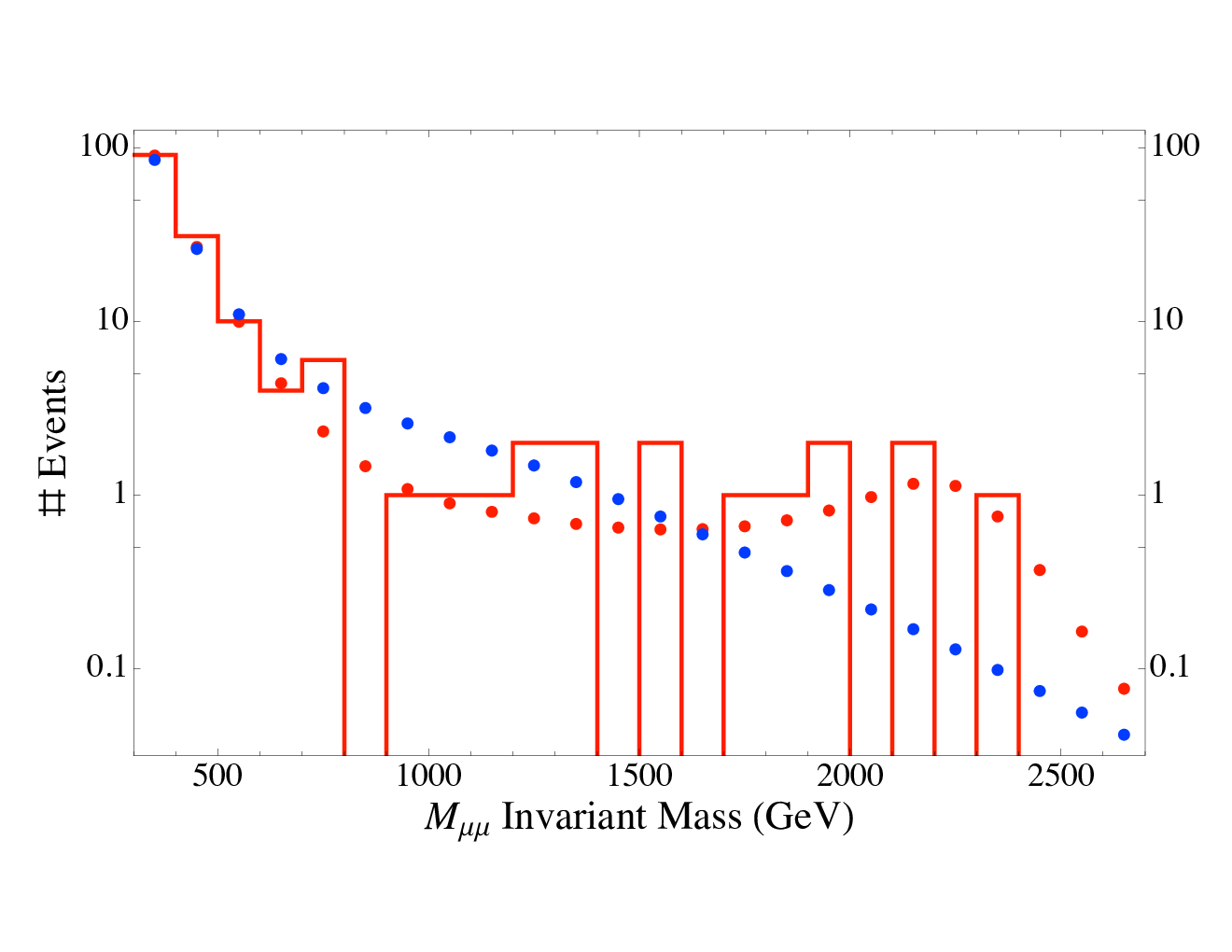
To illustrate the aforementioned difficulties in distinguishing different models of new physics through the invariant mass distribution, we ran two simulations showing possible outcomes of an experiment at and (see Fig. 3). We fit a resonance and a contact interaction to the data and, by sight, it seems that both might be consistent with the data up to statistical fluctuations. We want to see when it is possible to reliably distinguish between the two types of new physics, and how this discriminating capability varies with the parameters of the theory.11 1 If we take the resonance mass and coupling to be very large, we can integrate out the new physics and we do end up with a contact interaction. This, however, is not what we’re talking about here; rather, we are concerned about the case where the observed signal events are in the region around the resonance peak. In section 5, we will look at two methods for doing so. The first is relatively simple, looking for an absolute rise in the differential cross section. The second employs a statistic that is commonly used in experiments with few data points in each bin. We show that both of these methods can be used to distinguish resonances from contact interactions for most models predicting events in the early LHC running, though the more careful statistical method covers a larger range of parameters.

3 Models of new physics
In this section we define the two types of resonance models we use to demonstrate our methods, namely models of a new gauge boson, as well as RS models with at least one accessible KK graviton resonance. We also define the contact interaction models that we will compare with the resonances.
3.1 models
bosons commonly appear in physics beyond the SM (for a recent review, see [6]). The coupling of a to the SM can be written as
| (1) |
where
| (2) |
The charges will be discussed more in-depth shortly, although following [4], we will focus on that couple to and . We define the coupling in terms of the coupling by introducing the parameter :
| (3) |
We compute the differential and total cross sections to determine how these quantities scale with the model parameters. The partonic cross section has the form
| (4) |
where near the resonance or in the narrow width approximation, we have a partial width to states of mass
| (5) |
The partonic cross section evaluated at the pole is
| (6) |
and so the peak cross section decreases with higher , as expected. In a hadron collider, however, the partonic cross section, , is integrated against the corresponding parton luminosity function, , defined as follows:
| (7) |
where , to give the hadronic cross section
| (8) |
The hadronic cross section can be evaluated analytically only in the narrow width approximation, giving for CM energy
| (9) |
where . This is independent of the mass , except for the dependence on in the parton luminosity function. The parton luminosity function decreases monotonically with , as seen in Fig. 4.22 2 We probe the regime where the luminosity can no longer be taken as a simple power law: the total partonic luminosity from collisions at the LHC is approximately given by the expression .

phenomenology is dictated by the parameters and . In our analysis, we consider all values of these parameters consistent with experimental constraints. To observe higher-mass resonances, the coupling must be sufficiently large to compensate for the small parton luminosity, meaning that the models most visible during the early LHC running will be broad.33 3 Strictly speaking, this scaling argument only applies in the narrow width approximation, but we find a similar approximate power law scaling of hadronic cross section with even at large coupling, and our conclusion remains the same.
The only rigorous constraint on couplings comes from anomaly cancelation requirements. These can be satisfied in myriad ways - for instance, by the presence of hidden exotic states - but the simplest are “minimal models”, which consist purely of couplings to the SM plus right-handed neutrinos [3, 5]. The minimal models allow us to adequately study the various possibilities in a systematic way without introducing too many additional parameters, and we will restrict our attention to these. Anomaly cancelation then limits the overall charges to a linear combination of two independent charge assignments: hypercharge and . The hypercharge component leads to mixing with the and is tightly constrained by LEP measurements. In order to study models with stronger coupling to the SM, we will focus on of the type. Strictly speaking, the couplings will mix under renormalization group running [3], so models that unify with the SM at the GUT scale will generically see both types of charges, but this effect is small and, for the purposes of LHC phenomenology, we can ignore higher energies and simply examine the couplings at the TeV scale.
Although not as tightly constrained as a that couples to hypercharge, models are also strongly constrained by electroweak data if they are flavor-universal due to the constraints on electron-quark 4-fermion operators from LEP. If we only consider flavor-universal models, the LEP constraints are sufficiently strong to exclude all broad resonances with mass, and since these are the only type that will be visible in early LHC running, there will be no new parameter space open for exploration. A way around this is to couple the exclusively to muons in the leptonic sector [4, 7]; the theory will still be anomaly-free if the charges are . These non-universal models evade the bounds from LEP while giving large branching fraction to muon final states, enhancing the visible signal at the LHC. This means that there are regions of the parameter space that are accessible at the early LHC but that have not already been excluded at LEP. Our analysis generalizes that of [4] pertaining to coupling to , considering in particular the case of broad resonances and its experimental implications.
3.2 Brane RS models
Many of the best-motivated theories of new physics are those providing a solution to the hierarchy problem. One class of examples are RS models, in which the hierarchy between the Planck and electroweak scales is established with the addition of a warped extra dimension and the Higgs field confined to a brane at the IR scale [8]. For theories with the entire SM confined to the TeV brane, KK modes of the graviton could be detectable in early running if the TeV-brane energy scale is sufficiently low.
The couplings of higher KK modes of the graviton are suppressed by the warped scale . Here, is the AdS curvature scale and is the radius of the compact dimension. If the hierarchy problem is solved, then . The Lagrangian for the coupling of the KK graviton modes is
| (10) |
with energy-momentum tensor and -th KK graviton . The free parameters in this model can be taken to be and ; for phenomenological reasons, it is more convenient to exchange these for the dimensionless parameter and the first KK graviton mass
| (11) |
where is the first zero of the Bessel function . The subscript is used for the first mode because it is the graviton mode that will first appear at the LHC, and higher modes will likely be too heavy for discovery in the early running. These parameters are better-motivated from the standpoint of a resonance search and are directly analogous to the parameters and in models.
As with the , we compute the partonic and hadronic cross sections for lepton production–here via KK graviton exchange. For both gluon- and quark-initiated processes, the partonic cross section takes the form
| (12) |
where is the graviton self-energy. On-resonance, or in the narrow width approximation, the self-energy contribution can be simplified to give
| (13) |
where the graviton partial width to final states of mass scales as
| (14) |
The partonic cross section evaluated at the pole is
| (15) |
and the hadronic cross section is
| (16) |
where . This behavior is clearly analogous to that for a , and we are likewise led to the conclusion that strongly-coupled physics and broad resonances will appear first at the LHC.
Many analyses, beginning with [11], consider only RS models with coupling due to perturbativity constraints, restricting their studies to narrow resonances. This constraint, which comes from bounding the tree-level AdS curvature , neglects loop effects and is likely overly conservative.
3.3 Contact interactions
We now discuss contact interactions in more detail, as we saw in section 2 that, with small statistics, they might be confused with broad resonances. Contact interactions are convenient for parameterizing the low-energy behavior of new physics contributions. We consider generic contact interactions that are consistent with current experimental data and remain agnostic about possible UV completions of the theory.
The contact interactions most relevant to us are those involving quarks and muons. They are defined by a scale , and we use the parameterization [12]
| (17) |
where or 0 and can give chiral or axial/vector-like couplings.
Models with a vector-like coupling, denoted by VV, will have all couplings set to 1 or , each with the same sign. A left-handed model, denoted by LL, has only one non-zero coupling, , and thus only couples to left (right) handed quarks (anti-quarks) and muons (anti-muons). For these two models, the signs of the ’s determine the nature of the interference with the SM. The SM is recovered in the limit .
The contact interaction (17) arises from integrating out some spin-1 degrees of freedom. This seems like the best choice for mimicking a resonance, but at first glance, it may seem that a contact interaction generated by integrating out spin-2 degrees of freedom might do better at faking a graviton resonance. Such contact interactions, however, are dimension 8 and suppressed by extra powers of the scale . As a result, the event rate from such operators will not compete with the event rate from a broad resonance without running into serious conflict with existing experimental bounds. Thus, we find that even for RS gravitons, the interaction (17) is the best basis for comparison (we may also wish to consider scalar-type couplings, but as in the high energy limit, this only affects the angular distribution, we do not consider them here).
4 LHC dimuon cross sections
The current goal for early LHC running is at . To get a sense of the ultimate LHC reach, however, and also to see qualitatively what the possible outcomes of resonance searches may be at later times, we consider both the early run and also the cross sections at and , even though the analyses presented in this paper are mostly concerned with the first case. We consider the RS and models discussed in section 3 for different values of the mass and coupling. As anticipated in section 2, we demonstrate that the largest cross sections are in regions of parameter space with broad resonances, leading to the question of model discrimination between the broad resonance and a contact interaction that will be addressed in section 5.


We present our results for signal cross sections in Fig. 5 and 6 (for the flavor universal and non-universal cases, respectively), and our results for RS signal cross sections in Fig. 7. We mark contours of constant cross section, including the contours that will give 5 events at certain benchmark luminosities: at 7 TeV, at 10 TeV, and at 14 TeV. We indicate constraints using dashed lines. Details of the calculation and the relevant direct and indirect constraints follow later in this section. In the plots shown here, the regions of parameter space most ripe for exploration in the Drell-Yan channel at the LHC are those that couple strongly to muons, giving rise to broad resonances. The only exceptions are the models that are pure : since they couple universally to muons and electrons, the broad resonance regions are largely excluded by LEP. Indeed, even at high CM energy and luminosity, a will appear as a narrow resonance and the standard search strategies will apply.


We compute the differential cross sections at leading order in using the MSTW 2008 PDFs [13], with invariant-mass-dependent K-factors applied to quantify NLO QCD effects [14, 15]. Other necessary cuts due to detector geometry or triggering, for example and , are incorporated into the computation by employing an invariant-mass-dependent acceptance, following [3, 16]. The total cross section is then found by integrating the invariant mass distribution in some window. Typically, the width of this window is some multiple of the resonance width , but when we look at very broad resonances with , this will include events at very low invariant mass where SM background dominates. We therefore instead choose a lower cut-off for our window of , where is the invariant mass at which the signal differential cross section is twice as large than the background. Our upper cut-off for the window of integration will be , the CM energy of the collider.
We do not exclude any regions of parameter space solely for reasons of theoretical prejudice, but consider only experimental constraints. The most important ones for our study will be the bounds on 4-fermion operators from LEP [17] and the Tevatron [18]. The bounds from LEP in particular strongly constrain new physics coupling to electrons, such as the coupling to . One exception is the RS KK graviton that we have been discussing. It couples to the energy-momentum tensor and the lowest-dimension operator contributing to -channel graviton exchange is dimension 8, which is much less strongly constrained than the dimension-6 operators generated by massive vector exchange.
We also consider the strongest direct bounds on neutral resonances, which come from the Tevatron [19, 20]. These direct bounds do not extend much beyond 1 TeV because the Tevatron parton luminosity falls off very rapidly above this scale. Finally, we incoporate the bounds from muon experiments [21, 22, 23], although these do not strongly constrain RS models due to the cut-off dependence of the graviton contribution to , and so there are many values of and that can give the correct contribution. For models, the constraints from 4-fermion operators are stronger than those from .
5 Shape discrimination
5.1 Upturn analysis
As a simple first attempt at studying the shape of the distribution, we take advantage of one of the defining characteristics of a resonance: namely, the accompanying “bump”, or absolute rise and fall in the cross section. The background (or a contact interaction) will never actually give an increase in the cross section. We therefore look at regions of parameter space where we can, with confidence, say that there is a rise in the cross section over a flat background, indicative of a resonance with reasonable certainty. We find that for both KK gravitons and , the upturn analysis works for masses up to 1.5-2 TeV, and widths up to about 40% for and 90% for RS, depending on the mass.
To determine the reach of this analysis, we search for the local minimum of the differential cross section, as well as the corresponding point on the other side of the putative resonance peak. We then compute the integrated cross section in this region and compare it to a conjectured flat background. If we see a excess of events, then we know to a very high degree of confidence that we are seeing something new, since nowhere in the SM do we expect to see such behavior. We present our results for the upturn analysis at at the 7 TeV LHC in Fig. 8.
The behavior is as expected for narrow resonances, where nearly all of the signal events are above the upturn in cross section, and so the upturn analysis works everywhere that a normal counting experiment would. For very broad resonances (this definition depends on the precise model and resonance mass, but typically involves a ratio of width to mass that is larger than 50% for RS and 30% for ), the convolution with the falling parton luminosity function results in fewer events above the upturn (and, in some cases, no upturn at all), and they cannot be reached by this analysis.


This method is quick and easy but is overly conservative, since the background (and other, similar-looking types of new physics, such as contact interactions) are falling and not constant. Therefore, we are neglecting some broad resonances that should be distinguishable from background because they don’t show a particularly pronounced upturn in the differential cross section. We expect that the LHC reach for broad resonances should be more extensive than that shown here. Another shortcoming of this analysis is that it fails to account for statistical fluctuations in determining the start and endpoints for the integration window. An upturn could just as well come from a downward fluctuation in the lower-invariant-mass region, and our analysis does not consider this possibility.
5.2 Maximum likelihood method
We now present a more powerful method for discriminating resonances from contact interactions than the analysis presented above. We perform a full maximum likelihood anlysis [23] on the invariant mass distribution from a experiment. We simulate experiments assuming an underlying resonance as new physics, compare the maximum likelihood ratio obtained from resonance and contact interaction fits to the data, and determine over what parameters we can distinguish the two types of physics at the 95% confidence level based on the likelihood ratios. We outline details of our procedure here, and we present our results in section 5.3.
At very low statistics in each bin, as we expect to see if we restrict ourselves to high invariant mass events, we maximize the maximum likelihood function
| (18) |
where is the standard Poisson distribution and the are the means in each bin. Using the standard distribution to perform fits is not valid, as it assumes normally-distributed errors while the correct underlying distribution is Poisson [24]. The mean in each bin is found by integrating the differential cross section over the bin width. An unbinned analysis is also possible, but as the unbinned case can be obtained by taking the limit of the bin width to zero, we derive the results for a binned analysis and comment further on appropriate bin sizes in Appendix A.
The bin means are functionally dependent on the parameters of the theory; for instance, with contact interactions, we have , while for RS we have , with the index labeling bins.
With few high energy events, a better statistic than is [24]
| (19) |
where we define
| (20) |
which is the maximum likelihood ratio. The statistic has the property that , analogous to the . Maximizing is equivalent to minimizing , which is the criterion used for fitting, and good fits are characterized by small .
There are some important differences however from , which are seen when we apply the two statistics to a single bin (take to only have one value). Unlike the distribution, the mean and variance of is dependent on the mean of this bin [25]. For the , we always have an expectation value /d.o.f. (or /bin) of one, regardless of the bin mean. With small bin mean, we instead find . If we now sum over many bins, the total statistic will be dependent not only on the number of bins (like the ), but also on the means of those bins. Since the distribution is dependent on the bin means, which in turn are functions of the parameters of the theory, we have a different distribution of for each set of parameters. We therefore have no choice but to generate these through Monte Carlo simulations.
We will assume in everything that follows that the correct underlying new physics is a resonance model, and we will try to distinguish it from a contact interaction. To do so, we compare the values of that come from fitting resonance () and contact interaction () models to any simulated dataset. We compute
| (21) |
expecting for a dataset that looks more like a contact interaction and for a dataset that looks more like a resonance (the subscripts c and r stand for contact and resonance respectively).
Statistical fluctuations can make a contact interaction look more like a resonance and vice-versa, so it is not sufficient to examine the sign of . Our procedure for studying a resonance with mass and coupling is as follows:
- 1.
Generate data for a pseudoexperiment with at using a resonance model with parameters and .
- 2.
Perform fits of a resonance model ( and ) and a contact interaction with scale to the data , minimizing and respectively. The superscript shows that this is with respect to the data .
- 3.
Compute .
- 4.
To determine the values of that come from a contact interaction with scale faking a resonance, generate data based on a contact interaction with scale . Fit resonance and contact parameters to and compute . Repeat many times to generate a probability distribution over possible values of . The corresopnding cumulative distribution, given by the integral of , is .
- 5.
To distinguish the resonance in the data from a contact interaction at the 95% confidence level, we require . In words, if is bigger than 95% of the values based on fits to an underlying conctact interaction, then we can say with confidence that we have a broad resonance rather than a contact interaction.
The maximum likelihood ratio is well-known and used frequently in particle physics experiments in performing fits and determining the parameters of a theory from data, but we are here using it to directly compare two competing theories of new physics that may yield similar distributions of observables.
5.3 Results of statistical analysis
We now present the main results from our analysis. We apply the maximum likelihood analysis from the last section to the study of RS KK gravitons and non-universal discussed in section 3.44 4 In this section, we do not consider the flavor-universal case, as the LEP bounds imply narrow resonances in accessible regions of the parameter space at the LHC. We determine over what regions of parameter space we can distinguish such models from contact interactions. Examining Fig. 2, it is apparent that the destructively-interfering contact interactions will look most like a broad resonance. Whether it is LL or VV that most resembles the resonance depends on the nature of the resonance model’s coupling.
The analysis outlined in section 5.2 studies only a single arising from a single simulation of a resonance in of data. To quantify the effects of the statistical fluctuations over many different simulated experiments, we define reliability as the percentage of experiments in which we can distinguish a resonance from a contact interaction at the 95% confidence level. This essentially tells us the probability of being able to distinguish a resonance with at the LHC for various possible parameters.


Our results, showing the reliability curves for distinguishing resonances from contact interactions, are presented in Fig. 10 for RS and in Fig. 9 for the non-universal . Some of the key points from the figures that are true for both models are:
- 1.
It is most difficult to distinguish a resonance from a contact interaction that interferes destructively with the SM (in agreement with our earlier reasoning). For , it is the VV destructive contact interaction that is most likely to fake the resonance since that is the nature of the ’s own interference and coupling. For RS, where SM interference does not modify the total cross section, both destructive models do equally well, with only modest differences between the others.
- 2.
For narrow resonances (, ), the reliability curves track the cross section contours. Here, the relevant question is only the number of signal events required for detection: with five or more events, we can reliably distinguish between a resonance and contact interaction.
- 3.
For broad, low-mass resonances ( and TeV for RS, and TeV for ), we can universally discriminate between contact interactions and resonances because of the large number of events at . The effects of statistical fluctuations become negligible with many events.
- 4.
As expected, broad, high-mass resonances ( and TeV for RS, and TeV for ) are the hardest to distinguish from contact interactions at lower statistics. We find that it is still possible to detect broad resonances with confidence over most of the kinematically accessible parameter space, but the reliability of doing so diminishes when the width is greater than .


The analysis described above was done only for a single, isolated resonance. Generally, when we encounter strongly-coupled physics, we may find multiple resonances. We certainly expect to see additional resonances in the RS framework, namely the higher KK modes. The interference between resonances may be sufficiently high that we can no longer neglect the heavier modes, depending on resonance width and spacing.
As a check, we compute the contribution of multiple graviton KK modes (and their mutual interference) to the Drell-Yan process in RS. For , the effects of higher KK modes on the differential and total cross sections around are minimal. At higher coupling, we see enhancements to the cross section of up to %; most importantly, however, the shape is not distorted. Thus, these effects do not substantially change the outcome of the single-resonance analysis; the marginal increase in event rate will make at best make model discrimination slightly easier.
To better understand how the fitting procedure works, we plot the mean best-fit values of for RS resonances in Fig. 11, both for LL and VV destructive contact interactions. It is apparent that the best-fit values of are strongly correlated with the total number of events. The contact interaction most likely to fake a broad resonance is one that predicts the same number of events as the resonance, only with the events distributed in a different way. This is in accordance with our picture of unfortuitously distributed upward- and downward-fluctuations making a contact interaction look like a resonance.
In our analysis, we choose a bin size of 100 GeV, since that is on the order of the detector resolution for dimuon invariant masses around 1 TeV [26]. The range of invariant masses that we consider is 300 GeV to 4 TeV.55 5 Since the area around the peak is used to normalize the cross section and match the PDFs, we choose a lower value that safely avoids this region We have not included detector smearing effects. A discussion of the effects of including detector smearing and varying the bin size (justifying a binned analysis) is found in the Appendices.
5.4 Electrons and photons
The non-universal we have been considering evades the LEP bounds by coupling only to muons, and there will be no excess dielectron or diphoton final state events over the SM prediction. RS gravitons, however, couple to both electrons and photons, and these should make it easier to distinguish gravitons from contact interactions.
Electron and photon final states, like muons, have small SM backgrounds and are straightforward to detect. Depending on cuts imposed to minimize fake rates, detector efficiencies for electrons and photons can be as high as 60-85% [14]. The cross section for photon production by a KK graviton is twice that for muons, and so the total event rate increases by just under a factor of four when we include all channels (it is smaller than four because of the lower efficiencies for photons and electrons).

We plot our results for the RS cross section to electrons, muons, and photons in Fig. 12. We do not repeat the full statistical analysis and comparison to contact interactions because a) we expect the qualitative result to be the same, and b) it is difficult to systematically explore the full range of possible contact interactions, since we could have different coefficients for the operators involving different final states, etc. However, we do compare the cross section to that for muons alone and find that the new cross section contours are now shifted upward in mass by about 400 GeV. We therefore expect to be able to probe resonances to 400 GeV higher masses than if we relied only on muons, and the reliability regions would also shift accordingly, meaning that we have difficulty discriminating 2.8 TeV gravitons from contact interactions, rather than the 2.4 TeV gravitons we had with just muons.
6 Angular distribution
In this section we demonstrate how to use the pseudorapidity () distribution of the final state high muons to provide another handle in discriminating between models. We define a new variable called ellipticity, which measures how longitudinal the outgoing muons are in either the forward or backward directions, with no need to explicitly identify the direction of the quark vs. antiquark (as would be necessary for forward-backward asymmetry determination). We will see that this is a more efficient way to identify parity violation in new physics, particularly for broad resonances.
The SM violates parity, whereas new physics models may not. In a collider, this is encoded in the shape of the pseudorapidity distribution, as can be seen in Fig. 13, which shows the hadronic differential cross sections () for the standard model, where we have defined as the pseudorapidity of the outgoing from . The outgoing s are preferentially scattered forward relative to the quark in the SM, and since the quark could come from either proton, the distribution for the SM demonstrates a characteristic double peak structure. On resonance, new physics contributions that respects parity, such as the RS model, would wash out this effect, resulting in a transversely peaked distribution as shown on the right side of Fig. 13. Note that, at a collider, studying the forward backward asymmetry in the CM frame will not capture this effect since, without identifying the quark direction, the symmetry of the distribution would make the distinguishing peak structure cancel.
The shape of the distribution is significantly different than that of the distribution and requires explanation. The underlying hard interaction involves a valence quark whose momentum fraction is generally much larger than the antiquark’s and the resulting collision is boosted in the quark’s direction. Furthermore, the Standard Model preferentially scatters s into the same direction as the quarks as shown in Fig. 14, and when combined with the effect of the large boost, the resulting distribution is peaked away from the zero as shown by the dashed lines in Fig. 13. Since the valence quark could come from either proton, the distribution must be symmetric in and the two dashed curves are added to give the final double arched curve in Fig. 13. The cross section is more centrally peaked since the is preferentially scattered backwards from the quark and, after the boost, becomes more transverse with smaller rapidity. A collider would separately show the effects of parity violation in both of the distributions since these curves would are symmetric; however, the large boost at a collider magnifies the effect in the distribution while simultaneously diminishing the effect in .
Therefore, we study a new observable, the ellipticity (), to probe the shape of the distributions and we demonstrate its usefulness in discriminating between new physics models at the LHC. We calculate the ellipticity with the formula
| (22) |
where is the pseudorapidity of the outgoing . This quantity seeks to exploit the distinctive shape of the distributions. The end result is relatively insensitive to values of and , and so we have chosen , for this study. Ultimately, the value of could be optimized. Furthermore, studying a ratio has the usual advantage that some systematic uncertainties, such as the K-factor, integrated luminosity, PDF uncertainties, etc., will be common to both quantities and thus divide out.
We will also contrast ellipticity with the center-edge asymmetry [29] (), a related quantity based on the angular distribution in the CM frame that has been considered for spin determination. The center-edge asymmetry is defined using the quantity and is
| (23) |
This quantity attempts to exploit the differences in the distribution due the spin of the structure of the signal. For our study, we have taken and . A more thorough study of the variation of was carried out in [29]. Also, a modified version of center-edge asymmetry () was proposed in [30] that is based on instead of . Since , and behave similarly and any conclusions we draw for will also apply to . Notice that while and are defined analogously, with . We will demonstrate that, while and are both sensitive to the underlying spin structure, provides more discriminating power among models with different parity violating character.


Spin determination studies of narrow resonances have focused on the distribution of , where is the center of mass frame partonic scattering angle between the quark and the . Quantities that rely on differ from quantities that rely on for several reasons.
- •
depends on a difference of rapidities, which makes the quantity boost invariant. The boost magnifies the effects of parity violation and, since is boost invariant, the characteristic double peak feature of the standard model distribution is not present for .
- •
The forward-backward asymmetry () depends on and requires that one determine the direction from which the quark originated. This direction is not known in a collider a priori and the assignment of for each event is ambiguous. For very forward events, the boost required to bring the muons to the CM frame aligns with the direction of the quark’s momentum [28]. A rapidity cut to remove the low rapidity events would generate a sample for which we could measure ; however, it would also remove a majority of the signal events, which tend to be centrally peaked, and thus would not be useful until a significant amount of data has been recorded.
Another version of was proposed in [30] which probes differences in the distribution of . Since this variable is sensitive to the boost of the system, it behaves similarly to . Moreover, they showed that the inclusion of transverse events did not significantly affect the discriminating power of this variable and that it does not suffer the deficiency of the traditionally defined version of based on .
- •
cannot distinguish between models with the same spin structure, but with different amounts of parity violation. For example, the composite models being considered arise from integrating out a heavy spin one resonance, and so they share the same initial state and spin structure to the models. After convolving the partonic differential cross sections with the parton luminosity function, any parity violating effects are washed out as demonstrated in Fig. 15. These models are indistinguishable using . Conversely, not only can can distinguish models with similar spin structure, but with different amounts of parity violation.
- •
A difference in indicates either a different spin structure and/or coupling to initial state gluons. Thus can identify resonances mediated by an RS graviton, but it cannot distinguish between the rest of the models that we considered. In this regard, and are similar.


Figure 16: (left) and are shown for 1000 pseudo-experiments for TeV, fb-1 with GeV. The models shown are a RS model with GeV, (red), () model with GeV, (green), LL composite model with destructive interference and GeV (blue), and VV composite model with destructive interference and GeV (orange),
The calculation of the ellipticity is straightforward. The following expression gives the differential cross section in and , where is the rapidity of :
| (24) |
We have used the definitions
| (25) |
and the allowed region is
| (26) |
The two terms in braces in Eq. 24 represent the quark coming from either proton. The muon’s rapidity can be replaced with its pseudorapidity () at the energies we are considering, Inserting Eq. (24) into Eq. (22) gives the average value of the ellipticity. We similarly calculate the center-edge asymmetry using
| (27) |
which is then inserted to Eq. (23). Finally, when integrating over the invariant mass , one chooses different integration regions depending on the width of the resonance. When the resonance is narrow, events are selected in a single invariant mass bin around the resonances, which enhances signal over background. However, for broad resonances, there isn’t a convenient mass window that enhances the sample, and one is forced to include all of the events above a given invariant mass, , which will vary according to the shape and mass of the resonance. We have chosen the values of to be and GeV for the 7 and 10 TeV runs, respectively.
The appearance of (parity conserving) new physics above the mass cut will give larger values for the ellipticity due to the larger proportion of of centrally peaked s. For example, the representative RS model has a contribution to the DY cross section from the initial state gluons. These gluons tend to have comparable momentum fractions and so there isn’t a large boost as in the initial state; therefore, the distribution from tends to be centrally peaked. The contribution from shows a slight asymmetry, but it is dwarfed by the gluon contribution that washes out any distinctive shape.
The rather high invariant mass cut means there are only 100 or so events for 1 fb-1 at 7 TeV and so the observables will have large statistical uncertainties.


To model this uncertainty, a distribution of and was generated for 1000 pseudo-experiments for 1, 5 and 10 fb-1 at various CM energies. A representative set of distributions are shown in Fig. 16. The pseudo-experiments were generated with Pythia 8 [33, 34]. The LHC will only be able to make a single measurement and the distributions of Fig. 16 for the completing models are too similar for effective discrimination. There is some separation of the RS model from the rest, but to say the models are distinguishable is a bit of a stretch since there is significant overlap with the other distributions. We conclude that for masses greater than 1000 GeV, 1 fb-1 at 7 TeV is not enough integrated luminosity to be able to reliably distinguish among the models using these observables. Indeed, it is unlikely that any angular distribution observable will be able to discriminate models with so few statistics.
Discriminating power improves with more events, whether due to higher cross section (due to lighter new physics or higher CM energy) or higher integrated luminosity. The distributions are presented in Fig. 17 for TeV with 1 fb-1 (upper plots) and 5 fb-1 (lower plots) of luminosity for the same models as in Fig. 16, but with modified couplings and higher resonance masses or composite scales. The distributions in the lower plots show considerable separation indicating that for certain parameters, these models are distinguishable. For example, if the experiment measured a value of of 0.5, there is little chance that the LL composite model could be the underlying physics. The distributions shows clear separation between the RS model and the other spin 1 models, whereas the distribution distinguishes between the RS model, the LL composite model, and the parity conserving and VV composite models. This is a clear demonstration that has more sensitivity to parity violation than and will be a useful observable for model discrimination for broad resonances. Finally, and are complementary variables. Measuring will help discriminate between models of differing spin structure, after which a measurement of will further differentiate models based on their parity violating character. Once the models are distinguished, a more thorough investigation of the properties of the resonance can be performed.
7 Conclusions
In gearing up to study new physics at the LHC, we must consider the different features of the new collider. We have shown that, even in the first LHC run, its energy advantage over the Tevatron will allow it to probe new resonance physics, but only when couplings are sufficiently large to give sufficiently many signal events at relatively low luminosity. This has led us to the search for broad resonances. We have seen that careful statistical analyses will let us not only search for new resonances, but also discriminate them from contact interactions (as well as background).
We have furthermore considered angular distributions, a discriminator most likely to be useful only when the LHC runs at higher energy and luminosity. We demonstrated that the ellipticity is sensitive to parity-violation, even without knowing the quark direction, whereas the center-edge asymmetry is only sensitive to the spin structure of the interaction. Both observables provide complementary, useful, information.
8 Acknowledgements
We would like to thank Matthew Schwartz, Emily Thompson and Bob Cahn for helpful discussions about the project. We would also like to thank Ryan Kelley for his expert help with Pythia 8 and ROOT. LR is supported by NSF grant PHY-055611.
Appendix A Binning
We performed a binned analysis in section 5.3, which introduces uncertainties relative to an unbinned analysis that are proportional to the square of the bin size [27]. Nevertheless, we anticipate that the binned analysis gives comparable results to an unbinned analysis for the following reasons:


- 1.
The features of a broad resonance are on a scale , which is must larger than the 100 GeV bin width.
- 2.
With few events at high invariant mass, we never expect to see more than a single event (or two at most) per bin.
- 3.
At low invariant mass, where we expect more events, the distribution is dominated by SM interference, which we expect to be similar for different competing models of new physics (such as as vs. a destructively-interfering contact interaction. A counting experiment suffices in this region, as we don’t need high sensitivity to the shape of the invariant mass distribution here.
We present the results of a binned analysis with bin sizes 50 GeV and 25 GeV in Fig. 18, which are reduced relative to our standard 100 GeV bin size. It is evident that any differences between them are minor and do not affect our results qualitatively; therefore, the 100 GeV bin size is sufficiently small to give accurate results.
Reducing the bin size does have some advantages, however. In particular, the accuracy of the fit parameters is enhanced by performing an unbinned analysis, even though does not change much between them. In our case, however, we are not actually concerned with a precise determination of the resonance parameters, but whether characteristics of the invariant mass distribution allow us to generically distinguish it from other types of new physics, and this can be achieved accurately using a binned analysis.
Appendix B Detector smearing
The muon detectors at ATLAS and CMS have some finite resolution that introduces uncertainties into the invariant mass measurements. This has the tendency to smear the resulting distribution that comes out of the detector. The smearing should be applied both to the differential cross section used to generate the simulated data, as well as the contact and resonance distributions used to fit the data. This makes the whole simulation/fitting procedure much more computationally-intensive, particularly considering the number of fits that are required to scan over the parameter space and generate the distributions from the contact interactions.
Smearing tends to give otherwise narrow resonances a width of about the detector resolution, which at is still too small to leave any doubt that the new physics is a resonance. For broad resonances, however, it could further obscure the existing features of the resonance and make it look even more like a contact interaction. To determine the effects on our result, we repeated the analysis for a assuming Gaussian smearing using the detector resolution given by [26]. Our result is shown in Fig. 19.

The introduction of detector smearing does change the results, albeit by a relatively small margin (for broad resonances, we have loss in discriminatory power at fixed ). The detector effects do not, however, qualitatively change the results in any way, introducing only a small, horizontal shift in the reliability curves. Given that a proper analysis at ATLAS or CMS will require full-scale modeling of the detector, we are content to accept the non-smeared results as valid to within such a window.
References
- [1] C. W. Bauer, Z. Ligeti, M. Schmaltz, J. Thaler and D. G. E. Walker, Phys. Lett. B 690, 280 (2010) [arXiv:0909.5213 [hep-ph]].
- [2] R. Diener, S. Godfrey and T. A. W. Martin, arXiv:0910.1334 [hep-ph].
- [3] E. Salvioni, G. Villadoro and F. Zwirner, JHEP 0911, 068 (2009) [arXiv:0909.1320 [hep-ph]].
- [4] E. Salvioni, A. Strumia, G. Villadoro and F. Zwirner, JHEP 1003, 010 (2010) [arXiv:0911.1450 [hep-ph]].
- [5] L. Basso, A. Belyaev, S. Moretti, G. M. Pruna and C. H. Shepherd-Themistocleous, arXiv:1002.3586 [hep-ph].
- [6] P. Langacker, Rev. Mod. Phys. 81, 1199 (2008) [arXiv:0801.1345 [hep-ph]].
- [7] S. Davidson, S. Forte, P. Gambino, N. Rius and A. Strumia, JHEP 0202, 037 (2002) [arXiv:hep-ph/0112302].
- [8] L. Randall and R. Sundrum, Phys. Rev. Lett. 83, 3370 (1999) [arXiv:hep-ph/9905221].
- [9] T. Gherghetta and A. Pomarol, Nucl. Phys. B 586, 141 (2000) [arXiv:hep-ph/0003129].
- [10] K. Agashe, A. Delgado, M. J. May and R. Sundrum, JHEP 0308, 050 (2003) [arXiv:hep-ph/0308036].
- [11] H. Davoudiasl, J. L. Hewett and T. G. Rizzo, Phys. Rev. D 63, 075004 (2001) [arXiv:hep-ph/0006041].
- [12] E. Eichten, I. Hinchliffe, K. D. Lane et al., Rev. Mod. Phys. 56, 579-707 (1984).
- [13] A. D. Martin, W. J. Stirling, R. S. Thorne and G. Watt, Eur. Phys. J. C 63, 189 (2009) [arXiv:0901.0002 [hep-ph]].
- [14] ATLAS Collaboration, CERN-OPEN-2008-020 (2008).
- [15] Q. Li, C. S. Li and L. L. Yang, Phys. Rev. D 74, 056002 (2006) [arXiv:hep-ph/0606045].
- [16] CMS Collaboration, CMS PAS SBM-07-002 (2007).
- [17] J. Alcaraz et al. [ALEPH Collaboration and DELPHI Collaboration and L3 Collaboration and ], arXiv:hep-ex/0612034.
- [18] M. Titov [D0 Collaboration], PoS HEP2005, 314 (2006) [arXiv:hep-ex/0512006].
- [19] V. M. Abazov et al. [The D0 Collaboration], Phys. Rev. Lett. 104, 241802 (2010) [arXiv:1004.1826 [hep-ex]].
- [20] T. Aaltonen et al. [CDF Collaboration], Phys. Rev. Lett. 102, 091805 (2009) [arXiv:0811.0053 [hep-ex]].
- [21] C. S. Kim, J. D. Kim and J. H. Song, Phys. Lett. B 511, 251 (2001) [arXiv:hep-ph/0103127].
- [22] S. C. Park and H. S. Song, Phys. Lett. B 506, 99 (2001) [arXiv:hep-ph/0103072].
- [23] C. Amsler et al. [Particle Data Group], Phys. Lett. B 667, 1 (2008).
- [24] S. Baker and R. D. Cousins, Nucl. Instrum. Meth. 221, 437 (1984).
- [25] J. G. Heinrich, CDF/MEMO/CDF/CDFR/5718 v. 2 (2001).
- [26] O. Kortner, arXiv:0707.0905 [hep-ex].
- [27] R. Cahn, personal correspondence (2010).
- [28] M. Dittmar, Phys. Rev. D 55, 161 (1997) [arXiv:hep-ex/9606002].
- [29] P. Osland, A. A. Pankov, N. Paver and A. V. Tsytrinov, Phys. Rev. D 78, 035008 (2008) [arXiv:0805.2734 [hep-ph]].
- [30] R. Diener, S. Godfrey and T. A. W. Martin, Phys. Rev. D 80, 075014 (2009) [arXiv:0909.2022 [hep-ph]].
- [31] F. del Aguila, M. Cvetic and P. Langacker, Phys. Rev. D 48, 969 (1993) [arXiv:hep-ph/9303299].
- [32] T. G. Rizzo, arXiv:hep-ph/0610104.
- [33] T. Sjostrand, S. Mrenna and P. Z. Skands, JHEP 0605, 026 (2006) [arXiv:hep-ph/0603175].
- [34] T. Sjostrand, S. Mrenna and P. Z. Skands, Comput. Phys. Commun. 178, 852 (2008) [arXiv:0710.3820 [hep-ph]].