Whole Earth Telescope Observations of the subdwarf B star KPD 1930+2752: A rich, short period pulsator in a close binary.
Abstract
KPD 1930+2752 is a short-period pulsating subdwarf B (sdB) star. It is also an ellipsoidal variable with a known binary period just over two hours. The companion is most likely a white dwarf and the total mass of the system is close to the Chandresakhar limit. In this paper we report the results of Whole Earth Telescope (WET) photometric observations during 2003 and a smaller multisite campaign from 2002. From 355 hours of WET data, we detect 68 pulsation frequencies and suggest an additional 13 frequencies within a crowded and complex temporal spectrum between 3065 and 6343 Hz (periods between 326 and 157 s). We examine pulsation properties including phase and amplitude stability in an attempt to understand the nature of the pulsation mechanism. We examine a stochastic mechanism by comparing amplitude variations with simulated stochastic data. We also use the binary nature of KPD 1930+2752 for identifying pulsation modes via multiplet structure and a tidally-induced pulsation geometry. Our results indicate a complicated pulsation structure that includes short-period ( h) amplitude variability, rotationally split modes, tidally-induced modes, and some pulsations which are geometrically limited on the sdB star.
Keywords:
stars: general — oscillations: individual(KPD1930+2752)1 Introduction
Subdwarf B (sdB) stars are thought to have masses about 0.5M⊙ with thin (M⊙) hydrogen shells and temperatures from 22 000 to 40 000 K (Heber 1984; Saffer et al. 1994). Shell hydrogen burning cannot be supported by such thin envelopes and it is likely they proceed directly to the white dwarf cooling track without reaching the asymptotic giant branch (Saffer et al. 1994).
Pulsating sdB stars with periods of a few minutes (officially V361 Hya, and also known as EC 14026 or sdBV stars) were first observed by Kilkenny et al. (1997); nearly simultaneous to their predicted existence by Charpinet et al. (1996, 1997). The sdBV stars have pulsation periods ranging from 90 to 600 seconds with amplitudes typically near or below 1%. The pulsations are likely modes driven by the mechanism due to a diffusive iron-group opacity bump in the envelope (Charpinet et al. 1997, Jeffery & Saio 2007). Subdwarf B pulsators are typically found among the hotter sdB stars, with T34 000 K and . Reviews of this pulsation class include Reed et al. (2007a) for an observational review of 23 resolved class members and Charpinet et al. (2001) for a description of the pulsation mechanism. Another class of pulsating sdB stars have periods longer then 45 minutes, are likely mode pulsations and are designated V1093 Her, but commonly known as PG 1716 stars (Green et al. 2003; Reed et al. 2004a). General reviews of sdB stars and pulsators are Heber (2009) and Østensen (2009). Our target is a -mode, sdBV-type pulsator.
KPD 1930+2752 (also V2214 Cyg and hereafter KPD 1930) was discovered to be a variable by Billéres et al. (2000; hereafter B00), who obtained data during four nights within one week. Their longest run was five hours, yet within this limited data set, they detected 45 separate frequencies, which indicates that KPD 1930 is an interesting and complex pulsator. A velocity study confirmed the binary period and, using the canonical sdB mass of 0.5 , determined the companion mass to be (Maxted, Marsh, & North 2000). As the companion is not observed either photometrically or spectroscopically, it is likely a white dwarf, placing the mass of the system over the Chandrasekhar limit. A study by Ergma, Fedorova, & Yungelson (2001) suggested that the binary will shed sufficient mass to avoid a type Ia supernova and will merge to form a massive white dwarf. With a rich, unresolved pulsation spectrum and the opportunity to learn some very interesting physics via asteroseismology, KPD 1930 was chosen for observation by the Whole Earth Telescope (WET). KPD 1930 also has an infrared companion away (Østensen, Heber, Maxted 2005).
2 Observations
KPD 1930 was the target of the WET run Xcov 23. Nearly 355 hours of data were collected at 17 observatories from 15 August to 9 September, 2003. The individual runs are provided in Table 1. Overall, these data have an observational duty-cycle of 36% which is less than typical WET campaigns. Because of the crowded field, most of the data were obtained with CCD photometers, but some data were obtained with photoelectric (PMT) photometers. The photoelectric data were reduced in the usual manner as described by Kleinman, Nather, & Phillips (1996). The standard procedures of CCD image reduction, including bias subtraction, dark correction and flat field correction, were followed using IRAF packages. Differential intensities were determined via aperture photometry with the aperture optimized for each individual run with varying numbers of comparison stars depending on the field of view.
We will also examine a small multisite campaign that obtained data during July, 2002. In total, almost 45 hours of data were obtained from McDonald (the 2.1 m Otto Struve Telescope), San Pedro-Martir (1.5 m) and Suhora (0.6 m) observatories. Specifics of these runs are in Table 2.
| Run | Length | Date | Observatory | Run | Length | Date | Observatory |
|---|---|---|---|---|---|---|---|
| (Hrs) | UT | (Hrs) | UT | ||||
| t081403 | 5.5 | 15 Aug. | Mt. Cuba 0.4m | loi2708 | 3.0 | 27 Aug. | Loiano 1.5m |
| phot081503 | 6.4 | 16 Aug. | Mt. Cuba 0.4m | gv30808 | 5.8 | 27 Aug. | OHP 1.9m |
| phot081703 | 0.7 | 18 Aug. | Mt. Cuba 0.4m | a0688 | 2.0 | 28 Aug. | McDonald 2.1m |
| hunaug18 | 3.1 | 18 Aug. | Piszkesteto 1.0m | mdr245 | 0.9 | 28 Aug. | KPNO 2.1m |
| NOT_Aug19 | 7.8 | 19 Aug. | NOT 2.6m | haw28aug | 3.0 | 28 Aug. | Hawaii 0.6m |
| phot081903 | 6.5 | 19 Aug. | Mt. Cuba 0.4m | lulin28aug | 7.5 | 28 Aug. | Lulin 1.0m |
| hunaug19 | 4.3 | 19 Aug. | Piszkesteto 1.0m | turkaug28 | 2.5 | 28 Aug. | Turkey 1.5m |
| NOT_Aug20 | 8.6 | 20 Aug. | NOT 2.6m | jr0828 | 3.7 | 28 Aug. | Moletai 1.65m |
| lna20aug | 4.4 | 20 Aug. | LNA 0.6m | retha-0031 | 3.4 | 28 Aug. | SAAO 1.9m |
| phot082003 | 6.9 | 20 Aug. | Mt. Cuba 0.4m | phot082903 | 4.9 | 29 Aug. | Mt. Cuba |
| hunaug20 | 4.6 | 20 Aug. | Piszkesteto 1.0m | a0690 | 0.2 | 29 Aug. | McDonald 2.1m |
| hunaug21 | 4.8 | 21 Aug. | Piszkesteto 1.0m | mdr246 | 3.8 | 29 Aug. | KPNO 2.1m |
| NOT_Aug21 | 8.8 | 21 Aug. | NOT 2.6m | haw29aug | 3.0 | 29 Aug. | Hawaii 0.6m |
| lna21aug | 4.5 | 21 Aug. | LNA 0.6m | turkaug29 | 5.5 | 29 Aug. | Turkey 1.5m |
| lulin21aug | 7.0 | 21 Aug. | Lulin 1.0m | retha-0041 | 3.9 | 29 Aug. | SAAO 1.9m |
| NOT_Aug22 | 8.7 | 22 Aug. | NOT 2.6m | gv30809 | 5.7 | 29 Aug. | OHP 1.9m |
| lna22aug | 1.3 | 22 Aug. | LNA 0.6m | mdr247 | 6.8 | 30 Aug. | KPNO 2.1m |
| haw22aug | 1.0 | 22 Aug. | Hawaii 0.6m | haw30aug | 2.4 | 30 Aug. | Hawaii 0.6m |
| lulin22aug | 2.4 | 22 Aug. | Lulin 1.0m | turkaug30 | 4.3 | 30 Aug. | Turkey 1.5m |
| suh-114 | 3.9 | 22 Aug. | Suhora 0.6m | retha-0051 | 3.9 | 30 Aug. | SAAO 1.9m |
| gv30801 | 2.5 | 22 Aug. | OHP 1.9m | loi0830 | 0.1 | 30 Aug. | Loiano 1.5m |
| NOT_Aug23 | 6.5 | 23 Aug. | NOT 2.6m | mdr248 | 6.5 | 31 Aug. | KPNO 2.1m |
| lna23aug | 3.1 | 23 Aug. | LNA 0.6m | haw31aug | 2.9 | 31 Aug. | Hawaii 0.6m |
| haw23aug | 3.6 | 23 Aug. | Hawaii 0.6m | turkaug31 | 5.5 | 31 Aug. | Turkey 1.5m |
| lulin23aug | 6.8 | 23 Aug. | Lulin 1.0m | se0103q1 | 2.6 | 01 Sep. | SSO 1.0m |
| gv30803 | 1.1 | 23 Aug. | OHP 1.9m | turksep01 | 5.0 | 01 Sep. | Turkey 1.5m |
| lna24aug | 4.8 | 24 Aug. | LNA 0.6m | mdr249 | 3.6 | 02 Sep. | KPNO 2.1m |
| phot082403 | 6.9 | 24 Aug. | Mt. Cuba 0.4m | se0203q1 | 4.6 | 02 Sep. | SSO 1.0m |
| haw24aug | 0.5 | 24 Aug. | Hawaii 0.6m | turksep02 | 4.9 | 02 Sep. | Turkey 1.5m |
| gv30805 | 3.5 | 24 Aug. | OHP 1.9m | haw03sep | 2.3 | 03 Sep. | Hawaii 0.6m |
| phot082503 | 3.8 | 25 Aug. | Mt. Cuba 0.4m | se0303q1 | 4.5 | 03 Sep. | SSO 1.0m |
| haw25aug | 0.7 | 25 Aug. | Hawaii 0.6m | wise03sep | 6.0 | 03 Sep. | Wise 1.0m |
| lulin25aug | 0.2 | 25 Aug. | Lulin 1.0m | haw04sep | 2.4 | 04 Sep. | Hawaii 0.6m |
| suh-116 | 3.1 | 25 Aug. | Suhora 0.6m | se0403q1 | 4.6 | 04 Sep. | SSO 1.0m |
| gv30806 | 4.5 | 25 Aug. | OHP 1.9m | wise04sep | 3.8 | 04 Sep. | Wise 1.0m |
| phot082603 | 6.6 | 26 Aug. | Mt. Cuba 0.4m | hunsep04 | 1.7 | 04 Sep. | Piszkesteto 1.0m |
| a0684 | 0.5 | 26 Aug. | McDonald 2.1m | haw05sep | 2.5 | 05 Sep. | Hawaii 0.6m |
| a0685 | 0.3 | 26 Aug. | McDonald 2.1m | wise05sep | 7.0 | 05 Sep. | Wise 1.0m |
| lulin26aug | 7.0 | 26 Aug. | Lulin 1.0m | haw06sep | 2.2 | 06 Sep. | Hawaii 0.6m |
| retha-0020 | 0.7 | 26 Aug. | SAAO 1.9m | wise06sep | 7.0 | 06 Sep. | Wise 1.0m |
| gv30807 | 4.9 | 26 Aug. | OHP 1.9m | hunsep06 | 4.8 | 06 Sep. | Piszkesteto 1.0m |
| lna27aug | 3.5 | 27 Aug. | LNA 0.6m | haw07sep | 1.2 | 07 Sep. | Hawaii 0.6m |
| lulin27aug | 7.4 | 27 Aug. | Lulin 1.0m | hunsep07 | 4.6 | 07 Sep. | Piszkesteto 1.0m |
| retha-0021 | 3.7 | 27 Aug. | SAAO 1.9m | hunsep09 | 0.7 | 09 Sep. | Piszkesteto 1.0m |
| Run | Length | Date | Observatory | Run | Length | Date | Observatory |
|---|---|---|---|---|---|---|---|
| (Hrs) | UT | (Hrs) | UT | ||||
| 20710 | 3.5 | 10 July | Suhora 0.6m | A0302 | 4.0 | 14 July | McDonald 2.1m |
| 20711 | 1.8 | 11 July | Suhora 0.6m | A0304 | 3.9 | 15 July | Suhora 0.6m |
| A0296 | 2.0 | 11 July | McDonald 2.1m | 20717 | 5.9 | 15 July | McDonald 2.1m |
| 20712 | 5.3 | 12 July | Suhora 0.6m | sp1 | 2.4 | 17 July | Suhora 0.6m |
| A0300 | 0.3 | 13 July | McDonald 2.1m | 20720 | 2.2 | 17 July | S.P. Martir 1.5m |
| A0301 | 4.5 | 13 July | McDonald 2.1m | sp2 | 2.4 | 20 July | Suhora 0.6m |
| 20714 | 1.4 | 14 July | Suhora 0.6m | 20715 | 4.2 | 20 July | S.P. Martir 1.5m |
As sdB stars are substantially hotter than typical field stars, differential light curves are not flat due to atmospheric reddening. A low-order polynomial was fit to remove nightly trends from the data. Finally, the lightcurves were normalized by their average flux and centered around zero so the reported differential intensities are . Amplitudes are given as milli-modulation amplitudes (mma), with 10 mma corresponding to 1.0% or 9.2 millimagnitudes.

| Group | Inclusive dates | Res. | Limit |
|---|---|---|---|
| I | 15 Aug. - 9 Sep. | 0.45 | 0.44 |
| II | 18 Aug. - 7 Sep. | 0.60 | 0.31 |
| III | 19 - 23 Aug. | 2.69 | 0.44 |
| IV | 27 - 31 Aug. | 2.58 | 0.52 |
| V | 3 - 6 Sept. | 3.75 | 0.77 |
| VI | 2002, 10 - 21 July | 1.87 | 0.59 |
3 Analysis
3.1 Orbital Parameters
The largest variation in the lightcurve is caused by an ellipsoidal variation of the sdB star. In removing this variation to examine the pulsations, we can deduce some of the orbital properties. We defer attempting a complete binary solution to a work in progress (Pablo et al. private communication), but rather provide some basic information that are obvious from the data. Non-linear least-squares (NLLS) fitting to the data (2002 and 2004) provides a frequency of ellipsoidal variation of Hz. The binary period is twice that at or . Our value is within that found by B00 but outside the errors of the period determined by Geier et al. (2007; hereafter G07). G07 had 2900 spectroscopic data points unevenly scattered throughout four years while we have 36% coverage during 26 days in 2003 and hours spanning 7 days in 2002. As the epochs of our data overlap, period change can be ruled out and it is most likely that one (or both) of us are underestimating our errors. Figure 2 shows modified XCov 23 data folded over the binary period. The pulsations make the lightcurve very broad and it even appears that a pulsation frequency is an integer multiple of the binary period. However that is not the case, but rather there are many pulsation frequencies between 33 and 34 times the orbital frequency (see §3.2). To transform the broad pulsation-included lightcurve into a narrower, prewhitened form, we used our best data (Group II), prewhitened by all 61 pulsation frequencies. Then we phase-folded the data over the orbital period, did a 60-point ( s) smoothing, and fitted an additional three frequencies. We then prewhitened these three frequencies from the original, non-phase folded data, phase folded again, and smoothed by 60 ( s), 168 ( s), and 335 ( s) points. The differently smoothed data did not affect the maxima and minima of the orbital variations, and so we used the 335-point smoothed data, shown as a line in Fig. 2, to examine the ellipsoidal variations.

Using radial velocity data, G07 estimate the orbital inclination as . At that inclination, the white dwarf companion should eclipse the sdB star. An eclipse is shown for in Fig. 8 of G07 and using the orbital parameters of G07, we produced a simulated lightcurve with Binary Maker 311 1 See www.binarymaker.com.. Our simulation was not intended to fit the actual data, but rather to illustrate the eclipse shape. From the simulation, the eclipse duration would be s, or nearly three of our binned data points (at a binning of 335 points) with a depth of 0.2%. While the observed minima are uneven, the shape and depth do not match that of an eclipse. We can therefore rule out inclinations for which an eclipse should occur; namely , based on G07. The uneven minima indicates what would be expected based on the tidal distortion (gravity darkening). The gravity of the white dwarf makes the sdB star very slightly egg-shaped. When the marginally pointier end is facing us, the line-of-sight angle does not go as deep at one optical depth as it does when the blunter end is facing us. This produces a fainter minimum when the sdB is furthest from us and we view the slightly pointier end. A vastly exaggerated schematic of this is shown in Fig. 4 (a reconstructed image based on Fig. 2 of Veen et al. 2002). We fitted regions spanning 0.2 in phase with Gaussians to determine each maximum and minimum. The minimum at is % fainter than the other one and using detailed models, this information, along with the amplitude of the ellipsoidal variation should be sufficient to constrain the shape and limb darkening of KPD 1930. The uneven minima allows us to define closest approach of the sdB star, and like Maxted et al. (2000), we define that as the zero-point of the orbital phase.


The lightcurve maxima are also not quite even. Using the same Gaussian fitting technique, the maximum at , which is when the sdB component is traveling towards us, is % brighter then at , when the star is traveling away from us. Doppler boosting and Doppler shifting affects the flux by a factor of (G07; Maxted et al. 2000) which, using K1 from G07, should result in a Doppler brightening semi-amplitude of 0.11%. This is at the upper-limit of our measurement. Instead of using the measured velocity to deduce flux differences in maxima, two of us (SDK and HP) attempted to constrain the velocity from the lightcurve itself. Using low-pass filtering of the light curve, we obtained approximate values for the flux increase and converted that to velocity. The estimate of the maximum radial velocity is which is the same order as the radial velocity measurements of G07. The error estimate is the error of the fit to the light curve and does not include the (large) systematic error of the spectrum estimate. More on this measurement and its effects on the binary will be discussed in a future paper (Pablo et al. in preparation). So Doppler effects could be responsible for the difference in maxima. Interestingly, such special-relativistic effects have been detected in another sdB binary at the expected level (Bloemen et al., in press).
3.2 Pulsation analysis
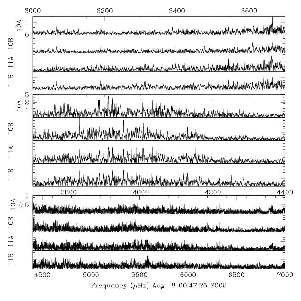
In a standard manner for long time-series data (i.e. Kilkenny et al. 1999; Reed et al. 2004b, 2007b), we analyzed the data in several different groupings. We can use these groups to examine frequency and amplitude stability, look for consistent frequencies, and amplitude variations. The groups are provided in Table 3 and pertinent sections of their temporal spectra (Fourier transforms; FTs) are shown in Figs. 5 and 6. Table 3 also lists the temporal resolution (defined as where is the run duration) and the detection limit determined for the range from 1 000 – 3 000 and 8 000 – 10 000 Hz. Group I data includes all of the XCov 23 data. Group II excludes noisy data, which is defined as a limit above 2 mma, and has been trimmed so that for any overlapping data, only the best quality data were kept. Groups III, IV, and V contain data obtained over 4 or 5 days of relatively good coverage during three different weeks of the 2003 campaign. Group VI is the 2002 small multisite campaign. Figure insets show the window functions, which are a single sine wave temporally sampled as the actual data. The central peak is the input frequency while other peaks are aliases which can complicate the data. Groups I and II are relatively well-sampled, with alias peaks less then 40% of the input amplitude whereas the remaining groups have obvious aliases that will contribute to the overall noise of the data.
A glance at the figures provides two simple observations: i) KPD 1930 is multiperiodic, pulsating in several tens of modes, confirming what was found in the discovery data (B00). ii) The pulsation frequencies are short-lived. This is evident in that the highest-amplitude peaks change between the shortest data sets (Groups III through VI) and the groups with the longest data sets (I and II) have the lowest amplitudes.


As peak amplitudes in FTs show a mixture of the median amplitude and effects of phase stability, prewhitening of the combined data sets could not be expected to accurately remove variations in amplitudes and/or phases (see Koen 2009 and Reed et al. 2007a). However, because of the frequency density shorter duration data sets would likely have unresolved frequencies. This does not mean that least-squares fitting and prewhitening are not of use, just that they need to be used with caution. We did the usual method of simultaneously fitting and prewhitening the data using non-linear least-squares (NLLS) software independently for all the groups in Table 3 until we could not discern peaks (as in Fig. 7). However, because of the rich pulsation spectrum we added an additional step. When searching the FT for pulsation peaks, we also plotted a window function made from the prewhitening information gathered for all fitted frequencies. In this manner, we could view cumulative windowing effects and better judge the impact of prewhitening on the FT. (A prewhitening sequence of Group IV’s data is provided as Fig. 1 in on-line supporting materials.)
Frequencies were deemed intrinsic to the star if they were detected in at least two Groups above the detection limits. Table 4 provides a list of detected pulsation frequencies. The first column lists a designation, the second gives the frequency from the highest temporal-resolution Group and the NLLS error in parentheses. Subsequent columns list the fitted amplitude from each group (NLLS error in parentheses) along with any pertinent notes: NF indicates that the frequency was not NLLS fitted; and frequencies fitted, but off by a daily aliases are noted as or for one daily alias away or or for two daily aliases away. The last column notes other frequencies that are within Hz of the daily alias as this could make prewhitening difficult, depending on the window function. Table 5 lists other frequencies that we suspect are intrinsic to the star, but did not meet our requirements. Figure 7 is an expanded FT for Group II’s data. Each two-panel section shows the original FT and the residuals after prewhitening. The dashed (blue) line is the detection limit. There are regions where the residuals remain higher then the detection limit because either NLLS fitting and prewhitening did not effectively remove all of the amplitude (most likely caused by amplitude and/or phase variations or another, unresolved frequency) or because remaining peaks were not observable in the original FT.
| Group | I | II | III | IV | V | VI | ||
| limit | 0.44 | 0.31 | 0.44 | 0.52 | 0.77 | 0.59 | ||
| Resolution | 0.45 | 0.60 | 2.69 | 2.58 | 3.75 | 1.87 | ||
| ID | Frequency | Amplitudes | Alias | |||||
| 3065.085 (49) | 0.70 (8) | 0.62 (8) | 0.56 (13) | 0.75 (13) | .. | 0.79 ( 14) | ||
| 3188.864 (44) | 0.68 (8) | 0.69 (8) | 0.62 (13) | 0.88 (13) | 0.61 (14) | |||
| 3308.382 (66) | 0.44 (8) | 0.45 (8) | NF | + | 0.63 (14)+ | |||
| 3422.386 (92) | .. | 0.32 (8) | .. | .. | .. | 0.56 (14)+ | ||
| 3489.608 (80) | 0.48 (8) | 0.38 (8) | .. | .. | .. | |||
| 3543.258 (60) | 0.52 (8) | 0.50 (8) | .. | 0.75 (13) | .. | .. | ||
| 3653.074 (54) | 0.55 (8) | 0.59 (9) | 1.13 (14) | .. | .. | .. | f8 | |
| 3664.968 (29) | 0.92 (9) | 1.10 (9) | .. | 1.09 (14) | 1.91 (24) | 1.25 (15) | f7 | |
| 3683.269 (63) | 0.41 (8) | .. | 0.95 (14) | .. | .. | 1.17 (16) | ||
| 3731.065 (38) | 0.84 (9) | 0.79 (8) | 1.40 (14)+ | 1.08 (15) | 1.15 (24) ++ | 1.06 (16)- | ||
| 3783.460 (17) | 1.51 (9) | 1.88 (9) | 2.35 (14) | 1.84 (15) | 1.52 (26) | 1.55 (19) | ||
| 3791.545 (41) | NF | 0.79 (9) | .. | NF | .. | 1.15 (19)+ | ||
| 3804.693 (41) | .. | 0.79 (9) | .. | .. | .. | 1.67 (17) | ||
| 3822.646 (39) | 0.70 (9) | NF | 1.28 (14)+NF | 0.90 (15)++ | 1.96 ( 26) | .. | ||
| 3852.709 (19) | 1.64 (9) | 1.90 (9) | 1.63 (14) | 2.27 (15) | NF | .. | f16 | |
| 3862.952 (34) | .. | 1.06 (9) | NF | .. | .. | 1.57 (16) | f15 | |
| 3908.614 (17) | 2.26 (11) | 2.09 (9) | .. | 3.76 (15) | .. | 2.85 (17)- | f18 | |
| 3920.717 (27) | 1.07 (10) | 1.40 (10) | NF | NF | NF | 1.04 (16) | f17 | |
| 3921.901 (28) | 1.22 (9) | 1.29 (9) | 2.40 (14) | .. | .. | .. | ||
| 3924.426 (26) | 1.30 (9) | 1.24 (9) | .. | .. | 3.94 (25) | .. | ||
| 3926.008 (25) | 1.11 (9) | .. | .. | .. | .. | 1.77 (16) | ||
| 3958.804 (35) | 0.66 (9) | 0.94 (9) | .. | .. | .. | .. | ||
| 3964.686 (30) | 0.93 (9) | .. | 1.72 (15) | .. | .. | .. | f24 | |
| 3974.320 (19) | 1.60 (9) | 1.68 (9) | 1.29 (15) | 1.97 (15) | 3.16 (25) | 1.76 (16) | f23 | |
| 3990.848 (29) | 0.65 (9) | 1.12 (9) | 1.04 (16) | 1.99 (15) | 1.74 (25) | .. | ||
| 4004.192 (25) | .. | 1.31 (9) | .. | .. | 2.01 (25) | .. | ||
| 4018.289 (27) | 1.22 (9) | 1.19 (9) | 1.85 (14) | 1.51 (15) | .. | 2.11 (16) | ||
| 4027.241 (27) | 1.04 (9) | .. | NF | 2.19 (16) | .. | .. | ||
| 4034.710 (31) | 0.90 (9) | .. | .. | 1.37 (16) | .. | .. | ||
| 4049.223 (29) | 0.86 (9) | 1.12 (9) | 1.23 (14) | 1.27 (15) | .. | .. | ||
| 4066.443 (33) | 0.84 (9) | 0.98 (9) | 1.21 (14) | .. | NF | .. | ||
| ID | Frequency | I | II | III | IV | V | VI | |
|---|---|---|---|---|---|---|---|---|
| 4120.459 (48) | 0.78 (9) | 0.65 (8) | .. | NF | 1.57 (24) | 1.41 (16)- | ||
| 4129.667 (32) | 0.69 (9) | 0.95 (9) | 1.34 (13) | .. | .. | 1.59 (16) | ||
| 4152.155 (33) | 0.55 (9) | 0.92 (9) | 1.02 (13) | 1.42 (14) | .. | .. | ||
| 4168.331 (36) | 0.92 (9) | 0.85 (8) | .. | 1.19 (14) | .. | 1.81 (15)+ | ||
| 4195.364 (51) | 0.65 (9) | 0.59 (8) | .. | 0.75 (14) | 1.03 (22) | 0.98 (14) | ||
| 4262.566 (69) | .. | 0.44 (8) | .. | 0.57 (14) | .. | .. | ||
| 4297.849 (58) | 0.44 (8) | 0.43 (8)- | 0.76 (17) | 0.57 (13) | .. | .. | ||
| 4453.34 (31) | .. | .. | 0.66 (13) | .. | .. | 0.62 (14)- | ||
| 4480.61 (57) | .. | .. | .. | .. | 0.78 (22) | 0.89 (14) | ||
| 4507.884 (62) | .. | 0.48 (8) | 0.50 (13)- | .. | NF | 0.57 (15)+ | ||
| 4524.708 (56) | 0.66 (8) | 0.53 (8) | 0.99 (13)- | 0.70 (13) | .. | 0.61 (14) | ||
| 4549.152 (69) | .. | 0.44 (8) | 0.49 (13) | .. | .. | .. | ||
| 4572.412 (42) | 0.61 (8) | NF | 0.51 (13)- | .. | 1.2 (22) | .. | ||
| 4716.271 (67) | NF | 0.45 (8) | .. | 0.60 (13)++NF | 0.98 (22) | NF- | ||
| 4769.657 (67) | 0.53 (8) | 0.45 (8) | 0.58 (14)- | .. | .. | .. | ||
| 4781.042 (94) | .. | 0.31 (8) | 0.67 (14) | .. | .. | .. | ||
| 4847.885 (84) | .. | 0.35 (8) | 0.55 (13) | .. | .. | 0.65 (14)- | ||
| 5184.009 (86) | .. | 0.34 (8) | .. | .. | .. | 0.64 (14) | ||
| 5207.451 (68) | NF | 0.44 (8) | NF | 0.67 (13) | .. | |||
| 5210.203 (78) | .. | 0.38 (8) | 0.50 (13) | .. | .. | .. | ||
| 5230.003 (41) | 0.63 (8) | .. | .. | .. | NF++ | 0.51 (14)++ | ||
| 5379.426 (79) | .. | 0.38 (8) | 0.57 (13) | .. | .. | .. | ||
| 5384.750 (83) | .. | 0.36 (8) | .. | 0.57 (13) | 0.71 (22) | 0.93 (14)+NF | ||
| 5416.641 (74) | .. | 0.40 (8) | 0.72 (13) | 0.65 (14)++ | .. | .. | ||
| 5451.930 (57) | .. | 0.53 (8) | 0.72 (17) | 0.73 (14) | NF | 0.58 ( 15) | ||
| 5459.529 (47) | 0.51 (8) | 0.64 (8) | 0.56 (17) | .. | 0.57 (15) | |||
| 5529.22 (37) | .. | .. | 0.54 (13) | .. | .. | .. | ||
| 5572.909 (74) | .. | 0.40 (8) | 0.51 (13) | .. | 0.72 (22)+ | .. | ||
| 5616.391 (65) | 0.51 (8) | 0.46 (8) | .. | 0.94 (13) | NF | .. | ||
| 5670.540 (79) | .. | 0.38 (8) | .. | 0.64 (13) | .. | 0.61 (14) | ||
| 5702.901 (51) | NF | 0.59 (8) | 0.98 (13) | .. | .. | 0.79 (15) | ||
| 5709.319 (79) | .. | 0.38 (8) | .. | .. | .. | 0.56 (15)+ | ||
| 5737.037 (83) | 0.35 (8) | 0.47 (13)+ | .. | .. | .. | |||
| 5938.582 (60) | 0.42 (9) | 0.54 (8) | .. | 0.74 (13) | .. | 0.51 (14)- | ||
| 5950.308 (68) | 0.44 (9) | .. | + | 0.61 (13) | .. | 0.74 (15) | ||
| 6319.148 (69) | 0.54 (9) | 0.44 (8) | .. | 1.03 (13) | 0.83 (22)+ | 1.40 (22 )+ | ||
| 6342.994 (62) | 0.52 (9) | 0.49 (8) | - | .. | .. | 0.75 (22) | ||
| ID | Frequency | I | II | III | IV | V | VI |
| Group | I | II | III | IV | V | VI | Alias | |
| 3448.361 (85) | .. | 0.35 (8) | .. | .. | .. | .. | ||
| 3885.715 (28) | 1.03 (10) | .. | .. | .. | NF | .. | ||
| 3995.235 (27) | 1.01 (9) | .. | .. | .. | NF | .. | ||
| 4030.437 (29) | 1.09 (9) | .. | .. | NF | NF | .. | ||
| 4232.67 (25) | .. | .. | 0.91 (14) | .. | .. | .. | ||
| 4246.23 (31) | .. | .. | 0.74 (14) | .. | .. | .. | ||
| 4307.84 (29) | .. | .. | 0.87 (17) | .. | .. | .. | ||
| 4897.000 (78) | .. | 0.38 (8) | .. | .. | .. | .. | ||
| 4949.582 (94) | .. | 0.31 (8) | .. | .. | .. | .. | ||
| 4965.63 (10) | .. | 0.36 (8) | .. | .. | .. | .. | ||
| 5140.42 (12) | .. | 0.25 (8) | .. | .. | .. | .. | ||
| 5769.48 (11) | .. | 0.28 (8) | .. | .. | .. | 0.55 (14) | ||
| 6083.547 (83) | .. | 0.35 (8) | + | .. | .. | .. |

3.3 The frequency content
In total, we detected 68 independent pulsation frequencies and 13 suspected ones. Here we summarize some generalities which will be used in subsequent sections. Only three frequencies are detected in all six data Groups while nearly is. Six other frequencies are detected in five data Groups and 13 are detected in four data Groups. 38 frequencies are within a 650 Hz region between 3650 and 4300 Hz. Unlike most sdBV stars, which contain several frequencies above 3 mma, KPD 1930 does not have any in the integrated data (Groups I and II). Only has an amplitude in all detections, though it is only detected in four Groups. 11 of the 68 frequencies have Group I amplitudes and these always have higher amplitudes in the shorter data sets (Groups III through VI), if detected. These simple observations again lead to the conclusion that pulsations of KPD 1930 are highly variable in amplitude and/or phase over the course of our observations. Combine that with the density in the main region of pulsations and accurate deciphering of the temporal spectrum will be difficult. Additionally, the pulsations in uncrowded regions have low amplitudes which will make them difficult to detect in short data sets.
4 Discussion
4.1 Comparison with the discovery data
By combining their four nights of data, B00 obtained a resolution of 1.89 Hz and their estimate of a mean noise level is 0.021%, giving their data a detection limit of 0.84 mma. By comparison, our XCov 23 data have better resolution and our detection limit is about half. Frequencies that match those of B00 are marked with a ⋄ in Tables 4 and 5 while those that are a daily alias away are marked with a ⋆. 26 of our 81 frequencies are related to the 44 listed in B00. Of the eight frequencies listed in B00 with amplitudes greater than 2 mma, seven are detected in our data. For comparison, there are 21 frequencies which we have detected in at least five of our Groups or have amplitudes in at least two groups (one of which must be Group I or II), and of these, eight are related to frequencies detected in B00. This also indicates a substantial amount of amplitude and/or phase change since the B00 observations.
4.2 Amplitude and phase stability
KPD 1930 shows characteristics similar to the sdBV star PG 0048+091 (Reed et al. 2007b), which has pulsation properties normally associated with stochastic oscillations. These properties include frequencies that are inconsistent between data sets and lower amplitudes in longer duration data. Of the 69 frequencies in Table 4, only , , and are detected in all six Groups of data, while is detected in five groups, with a peak just below in the sixth. Six more frequencies are detected and fitted in five of the six groups. Unfortunately, unlike PG 0048+091’s well-spaced frequencies, most of those in KPD 1930 are packed tightly between 3600 and 4200 Hz. Outside of this main region of power, the amplitudes are quite low, making detection difficult.
Despite these complications, we analyzed data sets of varying length with the goal of reaching timescales shorter than the timescale of amplitude and/or phase variations. Such data would be free of the resultant complications, allowing the amplitudes and phases to be more accurately measured. These could then be examined over the duration of our observations for changes. For the shortest possible time scale, we examined every individual run for which the detection limit was better then 2.0 mma; totaling 32 runs. We also created 13 daily data sets combining low-noise runs that were contiguous, or nearly so. The lengths of the daily data ranged from 7 to 27 hours, with a median value of 16.5 hours. Including the data for Groups III, IV, and V, we have data sets sampling time scales near 0.25, 0.67, and 4 days.
To resolve frequencies from individual runs and daily data sets, we selected frequencies from Table 4 that were isolated by at least Hz which included through , , , , through , and . We then attempted to fit amplitudes and phases for each of the frequencies for all of the data subsets. As expected, most of the fits failed as the pulsation amplitudes were well below the detection limits. Only for five frequencies were we able to fit phases and amplitudes to some of the shorter data sets. From the 48 data subsets, we fit 52 of a possible 480 phases and amplitudes for the five frequencies. Phases are determined as the time of first maximum amplitude after BJD=2452871.5 and converted to fractional phases by dividing by the period. In this manner, an error of 0.1 represents a 10% change in phase. The fractional phases and amplitudes are shown in Figs. 8 and 9 (and provided in tabular form in the on-line supporting materials). Horizontal bars indicate the time span of the data for the daily and Group sets. Note that some of the amplitudes are just below the detection limit. We include them because the peaks were fairly obvious in the FT and since the frequency is known, a lower detection limit is not unreasonable.


| All (54) | |||||
|---|---|---|---|---|---|
| #det | 7 | 16 | 8 | 14 | 16 |
| 0.79 | 1.07 | 1.43 | 1.33 | 1.04 | |
| 0.19 | 0.27 | 0.45 | 0.60 | 0.45 | |
| 0.24 | 0.25 | 0.31 | 0.45 | 0.43 | |
| 0.78 | 0.64 | 0.43 | 0.35 | 0.42 | |
| (%) | 4.3 | 12.4 | 19.7 | 17.8 | 17.1 |
| Individual runs (37) | |||||
| #det | 0 | 8 | 4 | 10 | 9 |
| .. | 1.11 | 1.72 | 1.47 | 1.20 | |
| .. | 0.29 | 0.45 | 0.64 | 0.51 | |
| .. | 0.26 | 0.26 | 0.44 | 0.43 | |
| .. | 1.67 | 2.35 | 2.75 | 2.41 | |
| .. | 0.66 | 0.73 | 0.53 | 0.50 | |
| .. | 0.62 | 0.35 | 0.31 | 0.37 | |
| .. | 1.05 | 0.65 | 0.76 | 0.87 | |
| .. | 0.79 | 0.72 | 0.41 | 0.59 | |
| .. | 0.41 | 0.26 | 0.17 | 0.18 | |
| .. | 0.70 | 0.47 | 0.40 | 0.43 | |
| .. | 0.53 | 0.53 | 0.22 | 0.29 | |
| (%) | .. | 14.6 | 26.0 | 19.2 | 13.6 |
| Daily runs (13) | |||||
| #det | 3 | 4 | 3 | 3 | 3 |
| 0.90 | 1.17 | 1.11 | 1.11 | 1.04 | |
| 0.05 | 0.13 | 0.26 | 0.25 | 0.13 | |
| 0.06 | 0.11 | 0.23 | 0.23 | 0.13 | |
| 0.95 | 1.28 | 1.35 | 1.40 | 1.17 | |
| 0.95 | 0.91 | 0.82 | 0.79 | 0.89 | |
| 0.69 | 0.59 | 0.55 | 0.41 | 0.42 | |
| 0.79 | 0.75 | 1.12 | 0.55 | 0.68 | |
| 0.65 | 0.54 | 0.45 | 0.33 | 0.38 | |
| 0.75 | 0.69 | 0.92 | 0.44 | 0.61 | |
| (%) | 4.0 | 14.5 | 8.0 | 15.2 | 12.2 |
| Groups III - VI | |||||
| #det | 4 | 4 | 1 | 1 | 4 |
| 0.71 | 0.88 | 1.24 | 0.61 | 0.71 | |
| 0.22 | 0.29 | .. | .. | 0.33 | |
| 0.31 | 0.33 | .. | .. | 0.46 | |
| 1.01 | 1.28 | 1.24 | 0.61 | 1.06 | |
| 0.70 | 0.69 | .. | .. | 0.67 | |
| 0.87 | 0.78 | 0.49 | 0.75 | 0.62 | |
| 0.61 | 0.54 | 0.49 | 0.75 | 0.42 | |
| (%) | 4.9 | 3.4 | .. | .. | 14.0 |
Table 6 examines the amplitude and phase properties organized by time domain. While is not detected in any individual runs, the phase is stable to within the errorbars. shows deviations of 12% and , , and have deviations all near 18%. Phase errors for individual measurements are under 10% (except for one) with an average of 5.0%. Phase variations are provided in Table 6 labeled as (%). While the deviations appear similar for , , and , has one discrepant value while , and appear phase variable, particularly from the individual runs (black circles in Fig 8). However none of the phases appear randomly distributed nor do they appear bimodal, which would be an indicator of unresolved frequencies.
The amplitudes show a larger variety. and are the most stable (the smallest ), but the amplitudes for are so small that it is not detected in any individual runs and only three of 13 daily runs. As such, it is clear that the number of detections will significantly affect amplitude stability as smaller, and therefore more deviant amplitudes will not have been measured. For these five frequencies, none are detected more than 30% of the time. Therefore our measure of amplitude variability, should be considered a lower limit. Likewise, the variations for , and must be higher then what we report as they have some relatively high amplitudes yet are not detected in all runs. For the amplitudes, temporally nearby runs can have different amplitudes and consistently, longer time domains have lower amplitudes. As these frequencies are reasonably separated from others for all of the timescales considered and their amplitudes do not appear bimodal, it is unlikely that beating plays a role in the amplitude variations. They are most likely intrinsic to the pulsations.
The original goal of this subsection was to determine the timescale of phase and amplitude variations. Indicators of that timescale are the standard deviations, the ratios between the average and maximum amplitudes, and comparing these between the sets. For example, if the timescale of variation is longer then a day, then the average and maximum values of the daily runs and the individual ones should be similar and should have near one. For , the average daily amplitude is slightly larger then that for the individual runs while that for the group sets is significantly smaller. This indicates that the timescale for amplitude variations is near to or longer than 16 hours but shorter than 72 hours.
4.3 Stochastic properties
An indicator for stochastic pulsations in solar-like oscillators is a ratio near 0.52 (Christensen-Dalsgaard et al. 2001). Pereira & Lopes (2005) also derived this ratio and were the first to apply it in testing whether pulsating sdB stars could be stochastically excited. Their results for the pulsating sdB star PG 1605+072, based on seven nights of data, indicated that those pulsations were driven rather than stochastically excited. The ratios for and are near to this value. However in solar-like oscillators the amplitude decay timescale is long compared to the re-excitation timescale, and so this ratio may not be a good indicator for sdBV stars. Other features that could indicate stochastic oscillations include significant amplitude variability, amplitudes that are reduced in longer-duration data sets (caused by phase variations), and matches with simulated stochastic data.
Just like for PG 0048+091, we produced Monte-Carlo simulations for stochastic oscillations with varying decay and re-excitation timescales appropriate for the various data sets and groups we have for KPD 1930. As there are many amplitude ratios to work with from Table 6, it was hoped that tight constraints for amplitude variations could be deduced by matching the simulations with the observations. However, such was not the case and the best we could do was produce loose timescales. The best results for indicate short amplitude decay timescales (four to six hours) and long re-excitation timescales (20 to 30 hours); those for indicate medium decay timescales (nine to 15 hours) and medium to long re-excitation timescales (12 to 27 hours); those for indicate short decay timescales (four to nine hours) and medium re-excitation timescales (eight to 16 hours); those for indicate short to medium decay timescales (four to 15 hours) and long re-excitation timescales (25 to 40 hours); and those for indicate short to medium decay timescales (four to 20 hours) and long re-excitation timescales (15 to 28 hours). The resultant timescales are fairly consistent in that the decays are always short compared to the re-excitations, but they are not nearly as clear as for PG 0048+091, certainly owing to the complexity of KPD 1930’s pulsation spectrum. However, the pulsation phases do not appear randomly distributed, as would be expected for stochastic oscillations. So we are left with some indications that stochastic processes may be present, and some contrary information against stochastic oscillations. From these data, we cannot discern between them.
4.4 Observed multiplets
From the ellipsoidal variations in KPD 1930, we can strongly infer it to be tidally locked, which means we also know the rotation period. In standard spherical harmonics, each can produce azimuthal values separated by the orbital frequency and the Ledoux constant (which is very small for modes in sdB stars)., we can search for multiplets to impose observational constraints on the mode degrees (). Table 7 lists multiplets detected to splittings of four times the orbital frequency of 121.7 Hz.As there are many pulsation frequencies related by a multiple of the rotation/orbital frequency, the order of the frequencies is the same as in Table 4 with the numbers in parentheses indicating the multiple of the rotation/orbital frequency between it and the previous (smaller) frequency. The leftmost frequency is just the lowest for each multiplet but has no significance otherwise.
| Des. | Designations of related frequencies | |
| 1 | f1: | f2 (1), f3 (1) |
| 1,1 or 3 | f4: | f6 (1), f8 (1), f17 (2), s72 (1), f34 (1) |
| 2 | f5: | f10 (2), f15 (1), f24 (1) |
| 2 or 4 | f7: | f27 (3), f37 (2), f41 (2) |
| 2 | f9 : | f13 (1), f21 (1), f30 (1), f35 (1) |
| 1 | f11: | f28 (2) |
| 1 | f12: | f29 (2) |
| 3 | f14: | f31 (2), s75 (2), f43 (2) |
| 1 | s70: | f33 (2) |
| 1 or 3 | f23: | f39 (4), f44 (1) |
| 2 | f25: | s73 (2) |
| 3 or 5 | s71: | f40 (4), f48 (3), f51 (3) |
| 1 | f26: | s74 (2) |
| 1 | f42: | f46 (2) |
| 2 | s76: | s79 (2), f55 (2) |
| 4 or 3 | s78: | f50 (2), f56 (2), f59 (1), f65 (3) |
| 2 | f49: | f61 (4) |
| 1 | f57: | f62 (2) |
| 1 | f60: | f64 (1) |
| 1 | f63: | f66 (2) |
4.4.1 Classical interpretation
In total, 61 of our 81 frequencies are related by a multiple of the rotation/orbital frequency. In a classical asteroseismological interpretation, we would assume the spin axis is aligned with the orbital axis and the stars are tidally locked. As such, we are viewing the spin axis close to equator-on, or an inclination near and the multiplets are caused by stellar rotation.
As each degree can have azimuthal orders, , the number of orbital splittings provides a minimum value and constrains where the is. For example, the triplet is best interpreted as an triplet with at . The multiplet beginning with has sufficient frequencies to warrant an interpretation. However, modes have low amplitudes caused by geometric cancellation, making such an interpretation unlikely. More feasible is that there are two multiplets with their outside components at a chance separation of nearly . Column 1 of Table 7 gives the minimum degree based on the number of orbital splittings. For entries with multiple possibilities, the most likely is given first. (On-line supporting material includes a color-coded figure showing the multiplets and a figure showing just the components with their corresponding degree.)
We can also use the pulsation amplitudes to place some constraints on the modal degrees. Using Groups I and II as a guide, all of the amplitudes are within a factor of 7 of each other, while most are within a factor of 4. Table 8 lists the geometric cancellation factors for azimuthal orders through for rotation axes of and . These factors indicate how much a pulsation amplitude would be reduced relative to a radial mode, which suffers no geometric cancellation. As column 2 indicates, for the classical interpretation, all of the modes have amplitudes reduced by factors less than 5 to 8, depending on orientation. This is roughly in agreement with the observed amplitude range. By contrast, all modes have amplitudes reduced by factors (except for depending on viewing angle). Since we don’t observe this range of amplitudes in KPD 1930, it is unlikely that these multiplets are being observed.
| Classical | Tipped | |
| 4.81 (2.44) | 1.69 (1.77) | |
| 1.20 (1.26) | 2.40 (2.52) | |
| 3.35 (4.70) | 4.18 (4.59) | |
| 7.28 (3.87) | 5.15 (5.65) | |
| 2.57 (2.82) | 5.48 (7.67) | |
| 48.2 (28.9) | 39.9 (45.9) | |
| 32.9 (70.6) | 860 (72.6) | |
| 51.7 (28.9) | 73.0 (57.8) | |
| 22.3 (25.7) | 68.1 (51.8) | |
| 32.9 (7,911) | 34.6 (41.8) | |
| 41.7 (4.81) | 7.46 (8.04) | |
| 30.0 (151) | 55.0 (45.9) | |
| 173 (21.4) | 64.2 (57.2) | |
| 81.4 (98.1) | 282 (218) |
Ignoring high-degree modes, there remains multiplets as evidence of 12 and four modes. There are also 20 frequencies which show no relations to other frequencies via an orbital overtone. These are all candidates for radial modes. As there is no geometric cancellation for radial modes, they would be expected to have some of the higher amplitudes. and all have amplitudes greater than 1 mma for all of their detections. Yet none of these have amplitudes significantly higher than the other frequencies. Therefore it is also possible they are modes with only one frequency visible.
4.4.2 Tipped-axis interpretation
Another interpretation would be that the pulsation axis is aligned with the tidal force of the companion. As described by Reed, Brondel, & Kawaler (2005), such a pulsation geometry would precess, completing a revolution every orbital period. The change in viewing pulsation geometry incorporates three additional pieces of information into the lightcurve which can be used to uniquely identify the pulsation degree and the absolute value of the azimuthal order . These are: a pattern of peaks in the FT of the integrated lightcurve; two or more flips in pulsation phase over an orbital period; and recovery of the “true” peak in the FT of the phase-separated data. As in Reed et al. (2005), we will not seek analytic solutions, but will use simulated data of precessing pulsation geometries to guide us. These simulations and any tipped-axis analysis make the assumption that spherical harmonics apply.
We begin by searching for patterns in the FT of the integrated data of KPD 1930. To guide our search, we produced simulated data for modes from through for an orbital/rotation axis of and a pulsation axis of relative to the rotation axis. This geometry seems reasonable for what we know of the orbital inclination and with tidal forces larger than the maximum Coriolis force. Changes of five to ten degrees in either axis make little difference in the patterns. The simulated FTs are shown in Fig. 10. The amplitudes are relative to the (radial) mode and along with the geometric cancellation factors of Table 8 indicate that high-degree modes are unlikely to be observed. The frequency patterns of Fig. 10 are what we are looking for in the observed data.

Eighteen of the multiplets from Table 4 match patterns from simulated tipped-axis pulsations22 2 These are shown schematically in Fig. 2 of the on-line supporting materials.. The next step is to divide the data into orbital regions of like and opposing pulsation phases (Reed et al 2005 show this procedure in detail) for the different modes. If the intrinsic frequencies predicted by the tipped-axis model are recovered, and their phases are opposite in appropriate data sets, this would be a reasonable indicator of a tipped pulsation axis. As can be seen in Fig. 10, the intrinsic frequency for tipped modes and will have a corresponding frequency in the combined data. As such, recovering the peak in the divided data is less important but detecting a phase shift of 0.5 will be vitally important for associating those frequency patterns with tipped pulsation modes.
We separated the data for Groups I through V into orbital regions of like and opposing phases appropriate for modes through and searched each Group not only for the frequencies predicted from the observed multiplets, but for any previously unobserved frequencies above the noise33 3 The phased data sets for Group II with and are shown in Fig. 5 of the on-line supporting materials.. The simplest data sets are those for as the orbit is divided into halves, with set A of going from an orbital phase of 0.0 to 0.5 and set B covering the other half. Those for are shifted by in phase. Table 9 provides the results of the search. Column 1 provides a unique mode identifier (with a corresponding identifier from Table 4 in parentheses, if there was one), column 2 the frequency, column 3 indicates the mode the data was phase-separated for and the remaining columns give the phase difference (set A minus set B) for each group.
| ID | Freq. | MODE | GI | GII | GIII | GIV | GV |
|---|---|---|---|---|---|---|---|
| 3913 | 1,0 | - | - | - | - | - | |
| 4008 | 1,0 | -0.50 (2) | 0.82 (2) | - | - | - | |
| 4113 | 1,0 | - | - | - | - | - | |
| 4126 | 1,0 | - | - | - | - | - | |
| 4647 | 1,0 | 0.55 (6) | -0.45 (5) | 0.27 (4) | -0.43 (6) | - | |
| 5581 | 1,0 | - | - | - | - | - | |
| 5831 | 1,0 | - | - | - | - | - | |
| 3187 | 1,1 | -0.55 (3) | 0.49 (5) | - | 0.46 (4) | - | |
| 3543 | 1,1 | -0.67 (3) | -0.64 (3) | -0.51 (4) | 0.39 (4) | 0.41 (4) | |
| 3853 | 1,1 | -0.08 (3) | -0.07 (2) | -0.16 (3) | -0.01 (2) | -0.13 (3) | |
| 4030 | 1,1 | -0.25 (2) | -0.26 (2) | - | -0.39 (2) | -0.26 (3) | |
| 4263 | 2,0 | - | 0.51 (2) | - | -0.31 (4) | - | |
| 5140 | 2,0 | - | - | - | - | - | |
| 3731 | 2,2 | -0.22 (2) | - | - | -0.27 (2) | - | |
| 3926 | 2,2 | - | - | - | - | - | |
| 5207 | 3,1 | - | - | - | - | - | |
| 4210 | 3,2 | -0.54 (5) | - | - | -0.63 (3) | - | |
| 4188 | 4,3 | - | - | - | - | - | |
| 4188 | 4,4 | 0.61 (4) | - | -0.47 (5) | - | - |
As anticipated considering the complexity of the data, the results are not straightforward. In the split data sets the aliasing is significantly worse and the pulsation amplitudes are very low. Evidence also suggests that amplitudes and phases are changing throughout the campaign.Most of the predicted frequencies are not detected. Those that are detected have amplitudes only marginally above the noise. But the strongest evidence will be consistent phase differences of one half in the various data sets. Frequency shows no phase shift between sets for all groups and so cannot be a tipped pulsation mode. Frequencies and have intermediate values, again indicating that they are likely not tipped pulsation modes, but rather that their phases are not stable over the course of the observations. Frequencies and are only detected in two of the five data sets, and while one phase difference is near one half, the other has an intermediate value. As is also seen in the integrated lightcurve, but shouldn’t be for an mode, it is unlikely a tipped mode. Frequencies , and do fit what we expect for tipped pulsations. is detected with a similar phase difference in all five groups, has consistent phase differences for the three data sets in which it can be detected, and has consistent phase differences in three of four detections. Additionally, is not detected in the integrated data, as should be the case. More surprising are the results for and , both of which are only detected in two of the five groups, but have phase differences near to one half. These modes are unlikely to be observed because the geometric cancellation factors are very high (73 and 282, respectively), meaning the intrinsic amplitudes would need to be much higher than the others. Monte Carlo simulations were produced with random phases between data sets. This could be appropriate for purely stochastic pulsations, but for driven pulsations, the phases should not be random at all, but rather close to a fixed number. As tipped pulsations have a phase shift of 0.5 which is very unexpected for driven pulsations, the significance of the simulations are somewhat startling. Our phase detections for and only occur in 0.1% of our simulations while those for occur 1.0% of the time. Those for and occur 6.7 and 4.9% of the time, repectively.
Of the 18 frequency multiplets in the combined data sets, three possess indicators for tipped pulsation modes. Nine have no detections at all, two have phase differences near zero, and two more have marginally appropriate phase differences, but would indicate modes that are unlikely to be detected because of geometric cancellation. Still, particularly for , which is not observed in the integrated data, the phase difference is a precise indicator for tipped pulsation modes. The chance of this occurring randomly is quite small.
4.5 Orbital dependence
While searching for tipped-axis pulsations, we stumbled upon the unexpected finding that some frequencies appeared to only occur for some stellar orientations44 4 These can be seen in Fig. 5 of the supporting materials.. So we divided the data up into four, eight, and 10 subsets according to orbital phase and examined the pulsation spectra of each. We found that quadrants, centered around the orbital phases 0 (QI), 0.25 (QII), 0.5 (QIII), and 0.75 (QIV) sufficiently differentiated the orbital dependence of the frequencies. Temporal spectra of Group II’s data, split into four quadrants are shown in Fig. 11. The dashed lines indicate likely intrinsic frequencies while the dotted lines are more likely aliases, with the arrows indicating which frequency they are an alias of.

It is obvious that there is an orbital dependence on some frequencies, particularly , which is clearly and only seen in QI. This most likely means that the pulsation geometry, as normally described by spherical harmonics, is more complex for these frequencies. Describing the pulsation geometry for such modes is beyond the scope of this paper, but we provide frequencies which have a detectable orbital dependence in Table 10. Outside of the main area of power, there is little sign of this uniqueness other then (5459) has a slightly higher amplitude in quadrant and (6319) is higher in quadrants and . Undoubtedly the lack of other detections is caused by low amplitudes combined with severe aliasing.
| ID | Freq. | QI | QII | QIII | QIV |
|---|---|---|---|---|---|
| 3787 | X | ||||
| 3799 | X | ||||
| 3831 | X | ||||
| 3865 | X | o- | |||
| 3882 | X | ||||
| 3963 | d+ | X | |||
| 4008 | X | ||||
| 4031 | X | o- | X |
5 Results
We have analyzed WET data spanning 26 days in August and September 2003, supplemented by 45 hours of multisite data obtained in July 2002. These data were used to examine the orbital properties and pulsation spectrum of the sdB+WD binary KPD 1930. We used the ellipsoidal variation to affirm the orbital period and folded the data over that period. No signs of eclipse were detected, constraining the inclination to . Additionally, we noted that the minima are uneven, indicating that KPD 1930 is very slightly asymmetric and marginally detect anticipated Doppler effects from possibly uneven maxima.
As implied from the discovery data (B00), we have found KPD 1930 to be an extremely complex pulsator with frequencies and amplitudes that can vary on a daily timescale. In these data, we confidently detect 68 pulsation frequencies and suggest a further 13. Of these, only 26 are related to frequencies observed by B00; a surprisingly small number that attests to KPD 1930’s pulsational complexity. Our WET data, which cover more than three weeks during 2003, have over four times better temporal resolution and one half the detection limit of B00.
We examined amplitude and phase stability by analyzing subsets of data over several time scales for well-separated frequencies. Unfortunately the low amplitude of these frequencies hampered our investigation and we were unable to detect them in most of the subsets. For the times we could detect them, we found the pulsation amplitudes to be fairly variable, although all ratios are short of the 0.52 used in solar-like oscillators to indicate stochastic oscillations (Christensen-Dalsgaard et al. 2001). The low ratio could be an artefact of only a few amplitude detections or caused by an amplitude decay timescale shorter then the re-excitation timescale. To investigate timescales we compared the observed amplitude ratios for several subsets with simulated stochastic oscillations. The simulations could easily fit the observed ratios and broadly found decay timescales near 12 hours and re-excitation timescales near 25 hours. As such, the pulsations do have some qualities normally associated with stochastic oscillations, however the phases are relatively stable which argues against stochastic oscillations. As such, it is possible that the amplitude variations have a different cause.
We have found 20 separate multiplets including up to 61 frequencies. Assuming the classical interpretation which aligns the pulsation axis with the rotation axis, these would indicate 12 , four , and/or possibly (but unlikely) four , two , and one modes. We also searched for indicators of a tidally-induced tipped pulsation axis which would precess with each orbit. While the complexities of the pulsations made searching for tipped modes difficult, three frequencies were found which indicated tipped modes and two further modes had some indications of tipped-modes, but were for and , which are unlikely to be observed. We also detected frequencies which only appeared during certain orbital phases, which indicates that some frequencies are affected by the slight asymmetry of the star. Figure 12 schematically shows these results with the arrow height indicating degree (except as noted below). Classically interpreted multiplet components are shown as solid arrows (with multiple possible frequencies connected by a horizontal line as in Fig. 10 and color-coded in the electronic version); modes from the tipped axis interpretation are shown as dashed arrows, with the value above the arrow; frequencies which only appear during certain orbital phases are shown as dotted arrows (at an arbitrary height of 1.5 since we have no indication of their degree). Any frequencies that were not involved in the above cases were (somewhat arbitrarily) deemed to be modes and are indicated as such in the figure with solid arrows. Note that the classically-interpreted mode which could have its component at 4453 or 4572 is marked with a question mark. This is part of the tipped multiplet and so if the tipped mode is correct, then the classical mode would be invalid. The small “3” and “2” under the axes are to indicate that there are three and two closely-spaced frequencies, all of which fit the conditions we ascribe to modes that would be unresolvable in the figure.

In the end, KPD 1930 is a star that incorporates a little bit of everything; many pulsation frequencies, multiplets, indications of a tidally-induced pulsation geometry, non-sphericity, relativistic Doppler effects, amplitude variations, and ellipsoidal variations, all wrapped up in a likely pre-Type Ia supernova binary. Unfortunately, all these effects complicate the analysis, making it a bit of an unruly mess. While we have tried to unravel it, our results indicate that even the WET fails to fully resolve the complexity of the pulsation spectrum and we can only imagine that perhaps MOST or Kepler-like data55 5 For information see http://www.astro.ubc.ca/MOST/ and http://astro.phys.au.dk/KASC/ would be required to improve this situation. Unfortunately, the Kepler field just misses KPD 1930. KPD 1930 remains a fascinating star that warrants further attempts to understand its complexities.
Acknowledgments
This material is based upon work supported by the National Science Foundation under Grant No. 0307480. Any opinions, findings, and conclusions or recommendations expressed in this material are those of the author(s) and do not necessarily reflect the views of the National Science Foundation. This research was supported in part by NASA through the American Astronomical Society’s Small Research Grant Program. MDR was partially funded by a Summer Faculty Fellowship provided by Missouri State University, would like to acknowledge HELAS travel funding, and thank Dr. Conny Aerts for helpful discussions. MAM, SLH, SP, JRE, and AMQ were suported by the Missouri Space Grant Consortium, funded by NASA. We would also like to thank several other observers who assisted with observing, including E. Brassfield, D. McLemore, J. Peacock, R. Knight, T. Kawasaki, E. Hart, N. Purves, A. Nishimura, M. Hyogo, and E. Rau.
References
- [1] Billéres M., Fontaine G., Brassard P., Charpinet S., Liebert J., & Saffer R.A. 2000, ApJ, 530, 441
- [2] Charpinet S., Fontaine G., Brassard P., Dorman B. 1996 ApJL, 471, 103
- [3] Charpinet S., Fontaine G., Brassard P., Chayer P., Rogers F.J., Iglesias C.A., Dorman B. 1997, ApJL, 483, 123
- [2001] Charpinet S., Fontaine G., Brassard P., 2001, PASP, 113, 775
- [4] Christensen-Dalsgaard J., Kjeldsen H., Mattei J.A. 2001, ApJ, 562, L141
- [5] Ergma E., Fedorova A.V., Yungelson L.R. 2001, A&A, 376, 9
- [6] Geen E.M., et al. 2003, ApJL, 583, 31
- [7] Geier S., Nesslinger S., Heber U., Przybilla N., Napiwotzki R., Kudritzki R.-P. 2007, A&A, 464, 299
- [8] Heber U., 2009, ARA&A, 47, 211
- [9] Heber U., Hunger K., Jonas G., Kudritzki R. P. 1984 A&A, 130, 119
- [10] Jeffery C. S., Saio H. 2007, MNRAS, 378, 379
- [11] Kilkenny D., Koen C., O’Donoghue D., Stobie R.S. 1997, MNRAS, 285, 640
- [12] Kilkenny D., et al. 1999, MNRAS, 303, 525
- [13] Kleinman S.J., Nather R.E., Phillips T. 1996, PASP, 108, 356
- [14] Koen Chris 2009, MNRAS, 392, 190
- [15] Maxted P.F.L., Marsh T.R., North R.C. 2000, MNRAS, 317, 41
- [16] Østensen R., 2009, Communications in Asteroseismology, 159, 75
- [17] Østensen R., Heber U., Maxted P., 2005, 14th European Workshop on White Dwarfs, ASP Conference Series, Vol. 334, 435, Ed. D. Koester, S. Moehler
- [18] Pereira Tiago M.D., Lopes Ilídio P., 2005, ApJ, 622 1068
- [19] Reed M.D., et al. 2004a, ApJ, 607, 445
- [20] Reed M.D., et al. 2004b, MNRAS, 348, 1164
- [21] Reed M.D., Brondel B.J., Kawaler S.D. 2005, ApJ 634, 602
- [22] Reed M. D., Terndrup D. M., Zhou A.-Y., Unterborn C. T., An D., Eggen J. R. 2007a, MNRAS 378, 1049
- [23] Reed M.D. et al. 2007b, ApJ 664, 518
- [1994] Saffer R. A., Bergeron P., Koester D., Leibert J., 1994, ApJ, 432, 351
- [24] Veen P. M., van Genderen A. M., van der Hucht K. A. 2002, A&A, 385, 619
6 Supporting Information
- •
Figure S1: Detailed prewhitening sequence of Group IV data between 3 600 and 4 250 Hz.
- •
Table S1: Pulsation phases and amplitudes for frequencies separated by Hz for individual runs, daily combined runs, and Groups of data.
- •
Figure S2: Schemitic of frequency spacings commensurate with the orbital frequency.
- •
Figure S3: Schematic associating pulsation frequencies with modes for traditionally-interpreted multiplets.
- •
Figure S4: Schematic associating pulsation frequencies with possible tipped modes.
- •
Figure S5: Pulsation spectra of Group II’s data, separated into opposing phases appropriate for and tipped pulsation axis modes.
7 On-line Only Material

| Phase () | Amplitude (mma) | ||||||||||
| Run: | |||||||||||
| not20aug | .. | 0.81 (6) | .. | -0.23 (7) | .. | .. | 0.8 (3) | .. | 0.8(3) | .. | 0.80 |
| not21aug | .. | 0.87 (4) | .. | .. | .. | .. | 1.1 (3) | .. | .. | .. | 0.79 |
| not22aug | .. | 0.77 (6) | 0.28 (4) | .. | .. | .. | 0.9 (3) | 1.3 (3) | .. | .. | 0.81 |
| not23aug | .. | .. | .. | .. | .. | .. | .. | .. | .. | .. | 0.82 |
| lulin27aug | .. | 0.98 (7) | .. | .. | 0.18 (7) | .. | 1.0 (4) | .. | .. | 1.1 (4) | 1.02 |
| a0688 | .. | .. | .. | 0.11 (3) | .. | .. | .. | .. | 2.8 (5) | .. | 1.48 |
| lulin28aug | .. | .. | .. | .. | 0.23 (9) | .. | .. | .. | .. | 0.9 (5) | 1.20 |
| gv30809 | .. | .. | .. | .. | 0.31 (4) | .. | .. | .. | .. | 1.4 (4) | 1.30 |
| turkaug29 | .. | .. | .. | .. | 0.34 (9) | .. | .. | .. | .. | 2.4 (1.4) | 1.98 |
| saao30aug | .. | 0.88 (4) | .. | .. | .. | .. | 1.7 (5) | .. | .. | .. | 1.81 |
| mdr248 | .. | 0.90 (7) | .. | -0.19 (4) | .. | .. | 1.0 (3) | .. | 1.3 (3) | .. | 1.01 |
| haw31aug | .. | .. | .. | -0.14 (5) | .. | .. | .. | .. | 2.1 (7) | .. | 1.81 |
| turkaug31 | .. | .. | .. | -0.13 (8) | .. | .. | .. | .. | 1.6 (8) | .. | 1.45 |
| turksep01 | .. | .. | -0.11 (9) | .. | .. | .. | .. | 1.5 (8) | .. | .. | 1.58 |
| turksep02 | .. | .. | .. | 0.32 (12) | 0.27 (13) | .. | .. | .. | 1.2 (9) | 1.2 (9) | 1.19 |
| wise03sep | .. | .. | 0.43 (6) | .. | .. | .. | .. | 1.6 (5) | .. | .. | 1.46 |
| haw05sep | .. | .. | 0.46 (5) | .. | .. | .. | .. | 2.4 (7) | .. | .. | 1.96 |
| hunsep06 | .. | .. | .. | 0.23 (6) | .. | .. | .. | .. | 1.3 (5) | .. | 1.82 |
| wise06sep | .. | 0.68 (5) | .. | 0.16 (8) | .. | .. | 1.4 (5) | .. | 1.4 (7) | .. | 1.48 |
| hunsep07 | .. | .. | .. | 0.01 (5) | .. | .. | .. | .. | 1.8 (6) | .. | 1.53 |
| aug25 | .. | .. | .. | 0.17 (5) | 0.48 (4) | .. | .. | .. | 1.0 (3) | 1.2 (3) | 1.41 |
| aug27 | .. | 1.06 (4) | .. | .. | .. | .. | 1.2 (3) | .. | .. | .. | 1.22 |
| aug28 | 0.40 (5) | 0.86 (3) | 0.52 (5) | -0.02 (7) | 0.24 (4) | 0.9 (3) | 1.3 (3) | 0.8 (3) | 1.4 (3) | 1.0 (3) | 1.10 |
| aug29 | 0.42 (5) | .. | .. | .. | 0.33 (4) | 1.0 (2) | .. | .. | .. | 0.9 (2) | 0.90 |
| aug30 | 0.34 (5) | 0.89 (4) | .. | -0.12 (5) | .. | 0.9 (3) | 1.0 (3) | .. | 0.9 (3) | .. | 0.96 |
| sep3 | .. | .. | 0.43 (5) | .. | .. | .. | .. | 1.1 (4) | .. | .. | 1.24 |
| sep4 | .. | .. | 0.36 (4) | .. | .. | .. | .. | 1.4 (4) | .. | .. | 1.30 |
| sep5 | .. | 0.70 (5) | .. | .. | .. | .. | 1.2 (4) | .. | .. | .. | 1.36 |
| Group III | 0.39 (4) | 0.83 (4) | .. | .. | -0.11 (7) | 0.5 (1) | 0.6 (1) | .. | .. | 0.3 (1) | 0.44 |
| Group IV | 0.37 (3) | 0.89 (3) | .. | 0.21 (4) | 0.22 (2) | 0.7 (1) | 0.9 (1) | .. | 0.6 (1) | 1.1 (1) | 0.52 |
| Group V | 0.39 (9) | 0.81 (3) | 0.40 (3) | .. | 0.11 (6) | 0.6 (2) | 0.8 (1) | 1.2 (2) | .. | 0.9 )2) | 0.77 |
| 0.04 | 0.12 | 0.20 | 0.18 | 0.17 | 0.19 | 0.27 | 0.45 | 0.60 | 0.45 | ||
| 0.24 | 0.25 | 0.31 | 0.45 | 0.43 | |||||||