Dimensional reduction and confinement from five dimensions
Abstract:
We study non-perturbatively five-dimensional gauge theories by means of the mean-field expansion on the lattice. On the anisotropic torus we show that a continuum limit can be defined where the anisotropy is a relevant parameter. The analysis of the static force supports the fact that the four-dimensional hyperplanes decouple from each other in the continuum limit. Clear signs of confinement are found in the static potential along the hyperplanes. We present first results from Monte Carlo simulations on the phase diagram.
WUB/10-27
June 14-19, 2010
Villasimius, Italy
1 Introduction and conclusions
Five-dimensional gauge theories are known to be perturbatively trivial, i.e. removing the ultraviolet cut-off leads to a free theory of photons [1]. The epsilon expansions [2, 3] suggests that there might be a non-perturbative ultraviolet fixed point, where the cut-off could be removed yielding an interacting theory, but this has been elusive so far in Monte Carlo simulations. Recently [4, 5] a ultraviolet fixed point was found within a mean-field computation. The computation is performed using the regularization of a pure gauge theory on an anisotropic Euclidean lattice and the continuum limit can be taken numerically at fixed physical box size and fixed anisotropy . The latter is defined as the ratio of the lattice spacing along the usual four dimensions and the one along the extra dimension, . The continuum limit can be taken when , a region of phase space that was not yet explored.
Monte Carlo simulations of five-dimensional gauge theories concentrated so far in the region where [6, 7], where dimensional reduction from five to four dimensions is expected to occur because the fifth dimension compactifies. The authors of [6] provided numerical evidence for the existence of a critical radius of the extra dimension ( is the string tension), below which the theory is four-dimensional.
In this talk we will concentrate on the regime . We first review the results of the mean-field computation adding to the data of [5] results from a larger lattice. Dimensional reduction seems to happen due to a localization mechanism. We will then present the exploration of the phase diagram through Monte Carlo simulations. So far we located a line of first order bulk phase transitions. It has been recently claimed in [8] that this phase transition could be of second order for parameters that are outside the range we investigate in this talk (see Fig. 4). We also see second order phase transitions due to compactification of one of the usual four dimensions. Detailed results of our Monte Carlo simulations will be presented in a forthcoming publication [9].
2 The mean-field laboratory for five-dimensional gauge theories
The mean-field expansion for gauge theories is reviewed in [10]. Path integral expectation values of operators over gauge links with action are replaced by integrals over complex matrices and Lagrange multipliers
| (1) | |||||
| (2) | |||||
| (3) |
The mean-field saddle point (or background) is defined by the minimization of the classical effective action in terms of constant fields
| (4) |
Gauge invariance is not broken, since arbitrary gauge transformations of the constant background solution Eq. (4) also fulfill the saddle point equations [10]. Corrections are calculated from Gaussian fluctuations around the saddle point solution
| and | (5) |
We impose a covariant gauge fixing on . In [11] it was shown that this is equivalent to gauge-fix the original links .
Our setup is a gauge theory formulated on a Euclidean lattice with anisotropic Wilson plaquette action [12]
| (6) |
where the sums run over all the four-dimensional and separately all the five-dimensional plaquettes counted with both orientations and is the product of the link variables around the plaquette . The dimensionless bare gauge coupling is defined through . We include the anisotropy factor . At tree level in the gauge coupling . Due to the anisotropy, the mean-field background is along directions and along the fifth dimension. We compute the following observables to leading order in the mean-field expansion [4]: the static potential along the four-dimensional hyperplanes orthogonal to the fifth dimension, the static potential along the fifth dimension, the scalar (or “Higgs”) mass and the vector gauge boson mass .


3 Dimensional reduction and continuum limit
The phase diagram of the theory can be mapped through the values of the mean-field background. There is a confined phase (, ), a layered phase (, ) and a deconfined phase (, ). By looking at the short distance behavior of we can decide, whether dimensional reduction occurs, in which case the potential has a four-dimensional Coulomb form (as opposed to a five-dimensional Coulomb law ). We identify two dimensionally reduced regions in the deconfined phase [4]: one at (compact phase) and one at close to the phase boundary with the layered phase (we call it the “d-compact” phase, where “d” stands for dual to the compact phase, since they are related by ). In the following, we study the properties of the d-compact phase.


In the left plot of Fig. 1 we show the results for the scalar mass at . It goes to zero when the phase boundary with the layered phase at is approached. It obeys the scaling law of the inverse correlation length of a second order phase transition with exponent fitted to . The value is the one of the four-dimensional Ising model and is in agreement with the analysis of [13]. The vector gauge boson mass is essentially independent of and (at leading order in the mean-field expansion) and depends essentially only on through with . This means that in the infinite volume limit the gauge boson is massless, i.e. no spontaneous gauge symmetry breaking takes place.
The existence of a second order phase transition means that we can take the continuum limit. We define lines of constant physics (LCP) by keeping
| and | (7) |
constant. We set and take the continuum limit by computations on a series of lattices . In the right plot of Fig. 1 we show the ratio of the static force along the extra dimension to the static force along the four dimensional hyperplanes. In order to plot physical quantities we need a way to set the lattice spacing, i.e. a quantity which is in principle measurable in four dimensions. Since the vector boson is massless, we cannot take . Instead we define a scale similarly to [14] from the static force through the equation . In Fig. 1 we plot the force ratio as a function of . We observed that the has a finite continuum limit [5]. The data shown in Fig. 1 suggests that goes to zero as . The interpretation of this result is that the system reduces in the continuum to a set of non-interacting four-dimensional hyperplanes. Dimensional reduction occurs through localization.
Since at short distance the static potential has a four-dimensional Coulomb form (see [5]), we fit it for on the lattices along the LCP Eq. (7) to the form
| (8) |
We do the fits locally, i.e. the coefficients , , and are functions of . In the range the coefficients have simultaneous plateaus, which we plot in Fig. 2 and Fig. 3 together with their continuum extrapolations linear in . We make the coefficients dimensionless by appropriate powers of . The continuum limit of the coefficient is consistent with the universal value of the Lüscher term [15, 16] in . This is our strongest evidence for dimensional reduction. In the continuum, we get a positive string tension together with a large and negative logarithmic correction. We cannot explain at the moment the origin of the negative logarithmic term, it hints to a dimensionally reduced theory in four dimensions different than a pure gauge theory, where such a term does not occur.

4 The phase diagram from Monte Carlo simulations
The mean-field calculation gives a consistent picture of a second order phase transition at anisotropy parameter . The next question is if this picture is validated by Monte Carlo simulations.
In Fig. 4 we summarize our Monte Carlo results for the phase diagram. We denote by symbols the location of phase transitions in the and plane. The red empty squares and the shaded line denote the bulk phase transition, which was first studied in [17]. It separates a confined phase, where the expectation values of the Polyakov lines are zero, from a deconfined phase, where they are non-zero along every direction and regardless of the lattice size. The bulk phase transition is of first order everywhere in the range of parameters plotted. This is signaled by a hysteresis curve in the plaquette observables and by a double peak in its susceptibility (when plotting simulation results from both cold and hot starts). In order to see this hysteresis the lattice volume has to be large enough and this is an issue in particular for the parameter region where (or ), since there one has to make the number of points in four directions large.
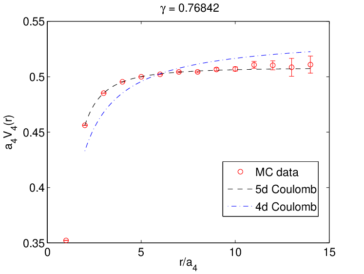
We study dimensional reduction by computing the static potential from Wilson loops. We distinguish two classes of Wilson loops, the ones in the four-dimensional hyperplanes (in directions , and ) and the ones along the fifth dimension in directions . From the former we extract the static potential , from the latter . In computing the Wilson loops, we use the multi-hit (or one-link) method [18] for the temporal links and two levels of HYP smearing [19] in directions for the spatial links. As an example, we show in Fig. 5 preliminary data for the static potential in the deconfined phase at . It can be perfectly fitted by a five-dimensional Coulomb potential.
At present, the only second order phase transitions that we could locate correspond to finite temperature (compactification). At we confirm the results of [6]. For the situation is shown in Fig. 4, in the region below the dashed line corresponding to . We located lines of phase transitions due to compactification of the fifth dimension or of the temporal dimension, signaled by a peak in the susceptibility of the respective Polyakov loop. As they evolve in the parameter space these lines cannot cross the line of the bulk transition, they will instead accumulate on it becoming always of first order. For the case of compactification with points (blue empty circles) or of with points (cyan filled circles), the finite temperature transition is always of second order if it happens far enough from the bulk phase transition. The order with points (green filled squares) is still under investigation. We will report in detail in [9].
Acknowledgments.
N.Irges thanks the Alexander von Humboldt Foundation and A. Rago the German Science Foundation (DFG) for support. The Monte Carlo simulations were carried out on the Cheops supercomputer at the RRZK computing centre of the University of Cologne and on the cluster Stromboli at the University of Wuppertal and we thank both Universities.References
- [1] K. R. Dienes, E. Dudas, T. Gherghetta, Grand unification at intermediate mass scales through extra dimensions, Nucl. Phys. B 537 (1999) 47.
- [2] H. Gies, Renormalizability of gauge theories in extra dimensions, Phys. Rev. D 68 (2003) 085015.
- [3] T. R. Morris, Renormalizable extra-dimensional models, JHEP 0501 (2005) 002.
- [4] N. Irges, F. Knechtli, Mean-Field Gauge Interactions in Five Dimensions I. The Torus, Nucl. Phys. B 822 (2009) 1, erratum: Ibid. 840 (2010) 438.
- [5] N. Irges, F. Knechtli, A new model for confinement, Phys. Lett. B 685 (2010) 86.
- [6] S. Ejiri, J. Kubo, M. Murata, A Study on the nonperturbative existence of Yang-Mills theories with large extra dimensions, Phys. Rev. D 62 (2000) 105025.
- [7] P. de Forcrand, A. Kurkela, M. Panero, The phase diagram of Yang-Mills theory with a compact extra dimension, JHEP 1006 (2010) 050.
- [8] K. Farakos, S. Vrentzos, Exploration of the phase diagram of 5d anisotropic SU(2) gauge theory, [arXiv:1007.4442].
- [9] F. Knechtli, M. Luz, A. Rago, in preparation.
- [10] J. -M. Drouffe, J. -B. Zuber, Strong Coupling and Mean Field Methods in Lattice Gauge Theories, Phys. Rept. 102 (1983) 1.
- [11] W. Rühl, The Mean Field Perturbation Theory Of Lattice Gauge Models With Covariant Gauge Fixing, Z. Phys. C 18 (1983) 207.
- [12] K. G. Wilson, Confinement of Quarks, Phys. Rev. D 10 (1974) 2445.
- [13] B. Svetitsky, L. G. Yaffe, Critical Behavior At Finite Temperature Confinement Transitions, Nucl. Phys. B 210 (1982) 423.
- [14] R. Sommer, A New way to set the energy scale in lattice gauge theories and its applications to the static force and in SU(2) Yang-Mills theory, Nucl. Phys. B 411 (1994) 839-854.
- [15] M. Lüscher, K. Symanzik, P. Weisz, Anomalies of the Free Loop Wave Equation in the WKB Approximation, Nucl. Phys. B 173 (1980) 365.
- [16] M. Lüscher, Symmetry Breaking Aspects of the Roughening Transition in Gauge Theories, Nucl. Phys. B 180 (1981) 317.
- [17] M. Creutz, Confinement and the criticality of space-time, Phys. Rev. Lett. 43 (1979) 553.
- [18] G. Parisi, R. Petronzio, F. Rapuano, A Measurement of the String Tension Near the Continuum Limit, Phys. Lett. B 128 (1983) 418.
- [19] A. Hasenfratz, F. Knechtli, Flavor symmetry and the static potential with hypercubic blocking, Phys. Rev. D 64 (2001) 034504.