Diassociative algebras and Milnor’s invariants for tanglesThanks: The second author was partially supported by the ISF grant 1343/10
Abstract.
We extend Milnor’s -invariants of link homotopy to ordered (classical or virtual) tangles. Simple combinatorial formulas for -invariants are given in terms of counting trees in Gauss diagrams. Invariance under Reidemeister moves corresponds to axioms of Loday’s diassociative algebra. The relation of tangles to diassociative algebras is formulated in terms of a morphism of corresponding operads.
Key words and phrases:
tangles, -invariants, planar trees, dialgebras, operads2010 Mathematics Subject Classification
57M25; 57M27; 18D50; 16S371. Introduction
The theory of links studies embeddings of several disjoint copies of into and thus has to deal with a mixture of linking and self-knotting phenomena. The theory of link-homotopy was developed by Milnor [7] in order to isolate the linking phenomena from the self-knotting ones and to study linking separately. A fundamental set of link-homotopy invariants is given by Milnor’s invariants [7] with non-repeating indices . Roughly speaking, these describe the dependence of the -th parallel on the meridians of the components. The simplest invariant is just the linking number of the corresponding components. The next one, , detects Borromean-type linking of the corresponding 3 components and together with the linking numbers classify 3-component links up to link-homotopy.
There is no semi-group structure defined on multi-component links such as one existing for knots. Namely, connected sum, while well-defined for knots, is not defined for links. On the level of invariants, this is manifested by a complicated recurrent indeterminacy in the definition of the -invariants (reflected in the use of notation , rather than ). Introduction of string links in [3] remedied this situation, since connected sum is well-defined for string links. A version of -invariants modified for string links is thus free of the original indeterminacy; to stress this fact, we use the notation for these invariants from now on. Milnor’s invariants classify string links up to link-homotopy ([3]).
1.1. Brief statement of results
Tangles generalize links, braids and string links. We define Milnor’s invariants for tangles with ordered components along the lines of Milnor’s original definition, that is in terms of generators of the (reduced) fundamental group of the complement of a tangle in a cylinder, using the Magnus expansion.
On the other hand, tangles may be encoded by Gauss diagrams (see [10, 2]). We follow the philosophy of [10] to define invariants of classical or virtual tangles by counting (with appropriate weights and signs) certain subdiagrams of a Gauss diagram. Since subdiagrams used in computing these invariants correspond to rooted planar binary trees, we call the resulting invariants tree invariants.
Invariance of tangle diagrams under Reidemeister moves gives rise to several equivalence relations among the corresponding trees. We study these relations and find (Theorem 3.3) that they could be interpreted as defining relations of a diassociative algebra. The notion of diassociative algebra was introduced by Loday [6]. A diassociative algebra is a vector space with two associative operations – left and right multiplications. The five defining axioms (equation 2) of diassociative algebra describe invariance under the third Reidemeister move.
We explicitly write out the linear combinations of trees used in computing invariants of degrees 2,3 and 4. In particular, tree invariants and are computed and subsequently shown to coincide with the corresponding Milnor invariants.
Then we discuss the properties of tree invariants of (classical or virtual) tangles. In particular, we study their dependence on orderings and orientations of strings. Moreover, we show that these invariants satisfy certain skein relations, reminiscent of those satisfied by the Conway polynomial and the Kauffman bracket. The skein relations for Milnor invariants were determined by the second author in [8]. Similarity of skein relations of tree invariants to Milnor’s invariants allows us to show that tree invariants coincide with Milnor’s -invariants when . This also allows us to extend Milnor’s -invariants to virtual tangles.
To describe the operadic structure on tangles we introduce the notion of a tree tangle. For tree tangles there is an appropriate operation of grafting, which allows us to define the operad of tree tangles. We show that there is a map from tangles to tree tangles by an operation called capping. We describe a morphism of operads between the operad of tree tangles and the diassociative algebra operad .
The paper is organized in the following way. In Section 2 the main objects and tools are introduced: tangles, Milnor’s -invariants, and Gauss diagram formulas. In Section 3 we review diassociative algebras and introduce tree invariants of tangles and prove their invariance under Reidemeister moves. Section 4 is devoted to the properties of the invariants and their identification with the -invariants. Finally, in Section 5 we discuss the operadic structure on tree tangles and the corresponding morphism of operads.
The authors are grateful to Paul Bressler, Frédéric Chapoton and Jean-Louis Loday for stimulating discussions, and to the French consulate in Israel for a generous travel support.
2. Preliminaries
2.1. Tangles and string links
Let be the unit disk in -plane and let , be some prescribed points in the interior of . For definiteness, we can chose the disk to have the center at and the points lying on the -axis.
Definition 2.1.
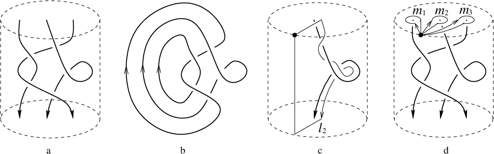
An (ordered, oriented) -tangle without closed components in the cylinder is an ordered collection of disjoint oriented intervals, properly embedded in in such a way, that the endpoints of each embedded interval belong to the set in . See Figure 1a. We will call embedded intervals the strings of a tangle. Tangles are considered up to an oriented isotopy in , fixed on the boundary.
We will always assume that the only singularities of (the image of) the projection of a tangle to the -plane are transversal double points. Such a projection, equipped with the indication of over- and underpasses in each double point, is called a tangle diagram. See Figure 1b.

String links form an important class of tangles which is comprised by -tangles such that the -th arc ends in the points , see Figure 2a. By the closure of a string link we mean the braid closure of . It is an -component link obtained from by an addition of disjoint arcs in the -plane, each of which meets only at the endpoints of , as illustrated in Figure 2b. The linking number of two strings of is their linking number in .
Two tangles are link-homotopic, if one can be transformed into the other by homotopy, which fails to be isotopy only in a finite number of instants, when a (generic) self-intersection point appears on one of the arcs.
2.2. Milnor’s -invariants
Let us briefly recall the construction of Milnor’s link-homotopy -invariants (see [7] for details, [5] for a modification to string links, and [8] for the case of tangles). We will first describe the well-studied case of string links, and then indicate modifications needed for the general case of tangles.
Let be an -component string link and consider the link group with the base point on the upper boundary disc . Choose canonical parallels , represented by curves going parallel to and then closed up by standard non-intersecting curves on the boundary of so that ; see Figure 2c. Also, denote by , the canonical meridians represented by the standard non-intersecting curves in with , as shown in Figure 2d. If is a braid, these meridians freely generate , with any other meridian of in being a conjugate of . For general string links, similar results hold for the reduced link group .
Given a finitely-generated group , the reduced group is the quotient of by relations , for any . One can show (see [3]) that is generated by , proceeding similarly to the usual construction of Wirtinger’s presentation. Let be the free group on generators . The map defined by induces the isomorphism of the reduced groups [3]. We will use the same notation for the elements of and their images in .
Now, let be the ring of power series in non-commuting variables and denote by its quotient by the two-sided ideal generated by all monomials, in which at least one of the generators appears more than once. The Magnus expansion is a ring homomorphism of the group ring into , defined by . It induces the homomorphism of the corresponding reduced group rings. In particular, for the case of being the link group of a link there is the homomorphism of reduced group rings .
Milnor’s invariants of the string link are defined as coefficients of the Magnus expansion of the parallel :
In particular, if passes everywhere in front of the other components, all the invariants vanish. Modulo lower degree invariants , where are the original Milnor’s link invariants [7].
The above definition of invariants may be adapted to ordered oriented tangles without closed components in a straightforward way. The canonical meridian of is defined as a standard curve on the boundary of , making a small loop around the starting point of (with ). A canonical parallel of is a standard closure of a pushed-off copy of (with ). See Figure 3. The only difference with the string link case is that for general tangles there is no well-defined canonical closure (some additional choices – e.g. of a marked component – are needed).

Remark 2.2.
Note that the invariants significantly depend on the order of indices and (e.g., in general ). Under a permutation , -invariants change in an obvious way: , where is the tangle with changed ordering: .
2.3. Gauss diagrams
Gauss diagrams provide a simple combinatorial way to encode links and tangles. Consider a tangle diagram as an immersion of disjoint copies of the unit interval into the -plane, equipped with information about the overpass and the underpass in each crossing.
Definition 2.3.
Let be a -tangle and its diagram. The Gauss diagram corresponding to is an ordered collection of intervals with the preimages of each crossing of connected by an arrow. Arrows are pointing from the over-passing string to the under-passing string and are equipped with the sign: of the corresponding crossing (its local writhe).
We will usually depict the intervals in a Gauss diagram as vertical lines, assuming that they are oriented downwards and ordered from left to right. See Figure 4.

The Gauss diagram of a tangle, , encodes all the information about the crossings, and thus all the essential information contained in the tangle diagram , in a sense that, given endpoints of each string, can be reconstructed from uniquely up to isotopy. Reidemeister moves of tangle diagrams may be easily translated into the language of Gauss diagrams, see Figure 5. Here fragments participating in a move may be parts of the same string or belong to different strings, ordered in an arbitrary fashion, and the fragments in and may have different orientations. It suffices to consider only one oriented move of type three, see [1, 9].

2.4. Virtual tangles
Note that not all collections of arrows connecting a set of strings can be realized as a Gauss diagram of some tangle. Dropping this realization requirement leads to the theory of virtual tangles, see [4, 2]. We may simply define a virtual tangle as an equivalence class of virtual (that is, not necessary realizable) Gauss diagrams modulo the Reidemeister moves of Figure 5.
The fundamental group may be explicitly deduced from a Gauss diagram of a tangle . It is easy to check that the fundamental group is invariant under the Reidemeister moves. Thus, the construction of Section 2.2 may be carried out for virtual tangles as well, resulting in a definition of -invariants of virtual tangles.
The only new feature in the virtual case is the existence of two tangle groups. This is related to a possibility to choose the base point for the computation of the fundamental group either in the front half-space (see Figure 2 and Section 2.2), or in the back half-space . While for classical tangles Wirtinger presentations obtained using one of these base points are two different presentations of the same group , for virtual tangles we get two different - the upper and the lower - tangle groups. See [2] for details. The passage from the upper to the lower group corresponds to a reversal of directions (but not of signs!) of all arrows in a Gauss diagram. Using the lower group in the construction of Section 2.2, we would end up with another definition of -invariants, leading to a different set of “lower -invariants” in the virtual case. We will return to this discussion in Remark 4.9 below.
2.5. Gauss diagram formulas
Definition 2.4.
An arrow diagram on strings is an ordered set of oriented intervals (strings), with several arrows connecting pairs of distinct points on intervals, considered up to orientation preserving diffeomorphism of the intervals.
See Figure 6. In other words, an arrow diagram is a virtual Gauss diagram in which we forget about realizability and signs of arrows.

Given an arrow diagram on strings and a Gauss diagram with intervals, we define a map as an embedding of into which maps intervals to intervals and arrows to arrows, preserving their orientations and ordering of intervals. The sign of is defined as . Finally, define a pairing as
and if there is no embedding of then For example, for arrow diagrams of Figure 6 and Gauss diagrams , shown in Figure 4, we have , and . We extend to a vector space generated by all arrow diagrams on strings by linearity.
For some special linear combinations of arrow diagrams the expression is preserved under the Reidemeister moves of , thus resulting in an invariant of (ordered) tangles. See [10] and [2] for details and a general discussion on this type of formulas. The simplest example of such an invariant is a well-known formula for the linking number of two components:
| (1) |
The right hand side is the sum over all maps of to . In other words, it is just the sum of signs of all crossings of , where passes under .
Remark 2.5.
Note that for string links one has
For general tangles, however, these two invariants may differ. For example, for a tangle diagram with just one crossing, where passes in front of , we have and depending on the sign of the crossing. This is a simple illustration of a general phenomenon: symmetries, which usually hold for classical links and string links, break down for tangles and virtual links. We will return to this observation in Section 3.
In the next section we introduce Gauss diagram formulas for a family of tangle invariants which includes all Milnor’s link-homotopy -invariants.
3. Tangle invariants by counting trees
In what follows, let , and .
3.1. Tree diagrams
Definition 3.1.
A tree diagram with leaves on strings numbered by and a trunk on -th string is an arrow diagram which satisfies the following conditions:
- •
An arrowtail and an arrowhead of an arrow belong to different strings;
- •
There is exactly one arrow with an arrowtail on -th string, if , and no such arrows if ;
- •
All arrows have arrowheads on strings;
- •
All arrowheads precede the (unique) arrowtail for each , as we follow the -th strand string in the sense of its orientation.
Note that the total number of arrows in a tree diagram is ; we will call this number the degree of . Our choice of the term tree diagram is explained by the following. Consider as a graph (with vertices being heads and tails of arrows and beginning and ending points of the strings). Removing all -strings where , and cutting off the part of each of the remaining strings after the corresponding arrowtail, we obtain a tree with leaves on the beginning of each -string with and the root in the endpoint of -th string. We will also say that is a tree with leaves on and a trunk on . See Figure 7, where some tree diagrams with , , are shown together with corresponding trees.

Note that every tree could be realized as a planar graph. The tree diagram is called planar, if in its planar realization the order of the leaves coincides with the initial ordering of the strings as we count the leaves starting from the root clockwise. For example, diagrams in Figure 7a are planar, while the one in Figure 7b is not. Let denote the set of all planar tree diagrams with leaves on and a trunk on and let .
3.2. Diassociative algebras and trees
Let the sign of an arrow diagram be , where is the number of right-pointing arrows in . Given a Gauss diagram of a tangle with the marked -th string, we define the following quantity, taking value in a free abelian group generated by planar rooted trees11 1 Note that this sum is always finite, since the Gauss diagram contains a fixed number of strings.:
While this formal sum of trees fails to be a tangle invariant, it becomes one modulo certain equivalence relations on trees. These relations turn out to be the axioms of a diassociative algebra (also known as associative dialgebra):
Definition 3.2.
([6]) A diassociative algebra over a ground field is a -space equipped with two -linear maps
called left and right products and satisfying the following five axioms:
| (2) |
Diagrammatically, one can think about a free diassociative algebra as follows. Depict products and as elementary trees shown in Figure 8a. Composition of these operations corresponds then to grafting of trees, see Figure 8b,c.


3.3. Tree invariants
Let denote the equivalence class of a planar tree in , and be the Gauss diagram of a tangle. Then is defined as
| (3) |
being the tree corresponding to the tree diagram . We call the tree invariant of a tangle which has as its Gauss diagram, since it satisfies the following
Theorem 3.3.
Let be an ordered (classical or virtual) tangle and let be a Gauss diagram of . Then is an invariant of ordered tangles.
Proof.
It suffices to prove that is preserved under the Reidemeister moves – for Gauss diagrams (Figure 5). Given a Gauss diagram , invariance of under and follows immediately from the definition of tree diagrams. Indeed, a new arrow appearing in has both its arrowhead and its arrowtail on the same string, so it cannot be in the image of a tree diagram . Hence the (3) rests intact under the first move. It is also invariant under the second move for the following reason. Two new arrows which appear in have their arrowtails on the same string, so they cannot simultaneously belong to the image of a tree diagram, while maps which contain one of them cancel out in pairs due to opposite signs of the two arrows.
It remains to verify invariance under the third Reidemeister move depicted in Figure 5. Denote by and Gauss diagrams related by . Note that there is a bijective correspondence between the summands of and those of . Indeed, since only the relative position of the three arrows participating in the move changes, all terms which involve only one of these arrows do not change. No terms involve all three arrows, since such a diagram cannot be a tree diagram. It remains to compare terms which involve exactly two arrows. Note that a diagram which involves two arrows can be a tree diagram only if the fragments participating in the move belong to three different strings. There is a number of cases, depending on the ordering of these three strings. Using for simplicity indices for such an ordering, we can summarize the correspondence of these terms in the table below.
![[Uncaptioned image]](1011.0117v2/table.png)
We see that invariance is assured exactly by the diassociative algebra relations, see Figure 9. For four orderings out of six the correspondence is bijective, while for the two last orderings, pairs of trees appearing in the bottom row have opposite signs (due to different number of right-pointing arrows), so their contributions to cancel out. ∎
4. Properties of the tree invariants
The tree invariant takes values in the quotient of the free abelian group generated by trees by the diassociative algebra relations. The equivalence class of a tree with trunk on depends only on the set of its leaves, so it is the same for all arrow diagrams in the set of all planar tree arrow diagrams with leaves on and trunk on .
Let be the coefficient of corresponding to trees with leaves on , namely, . For we set .
4.1. Invariants in low degrees
Let us start with invariants for small values of .
Counting tree diagrams with one arrow we get
| (4) |
Note that if is a string link .
For diagrams with two arrows we obtain
| (5) |
In particular, . Also, , where is the tangle with reflected ordering of strings.
Example 4.1.
Consider a tangle with corresponding diagram depicted in Figure 4 and let us compute using formula (5). The corresponding Gauss diagram contains three subdiagrams of the type , two of which cancel out, while the remaining one contributes ; there are no subdiagrams of other types appearing in (5). Hence, .
When an orientation of a component is reversed, invariants change sign and jump by a combination of lower degree invariants. For example, denote by the 3-string tangle obtained from by reversal of orientations of . Then,
But it is easy to see that , thus we obtain
Let us write down explicitly 3-arrow diagrams with trunk on the first string:
| (6) |
For diagrams with trunk on the second or third strings we have , . Finally, for we have , where is obtained from by the reflection of the ordering.
4.2. Elementary properties of tree invariants
Unlike -invariants discussed in Section 2.2 which had simple behavior under change of ordering (see Remark 2.2), tree invariants depend significantly on the order of and . Namely, if for some , , then, in general, is not directly related to . However, in some simple cases dependence of tree invariants on ordering and their behavior under simple changes of ordering and reflections of orientation can be deduced directly from their definition via planar trees:
Proposition 4.2.
Let be an ordered (classical or virtual) tangle on stringsand let , with .
- (1)
For we have
where and .
- (2)
Denote by the tangle with reflected ordering: , , where , so . Then
- (3)
Finally, denote by the tangle the tangle obtained from by cyclic permutation of strings of (that is, for and ), followed by the reversal of orientation of the last string . Then
Proof.
Indeed, a planar tree with trunk on consists of the “left half-tree” with leaves on and the “right half-tree” with leaves on . Thus the first equality follows directly from the definition of the invariants.
Also, the reflection of ordering simply reflects a planar tree with respect to its trunk, exchanging the left and the right half-trees and changing all right-pointing arrows into left-pointing ones and vice versa, so the second equality follows (since the total number of arrows is ).
Finally, let us compare planar tree subdiagrams in the Gauss diagram of and in the corresponding Gauss diagram of . Cyclic permutation of ordering, followed by the reversal of orientation of the trunk, establishes a bijective correspondence between planar tree diagrams with leaves on and trunk on and planar tree diagrams with leaves on and trunk on . Given a diagram , we can obtain the corresponding diagram in two steps: (1) redraw the trunk of on the right of all strings, with an upwards orientation; (2) reverse the orientation of the trunk so that it is directed downwards. See Figure 10.

Signs of these diagrams are related as follows: , where is the number of arrows with arrowheads on the trunk (since all such arrows become right-pointing instead of left-pointining). Now note that when we pass from to , the reflection of orientation of has similar effect on the signs of arrows, namely, the sign of each arrow in with one end on the trunk (and the other end on some other string) is reversed, so . These two factors of cancel out to give and the last statement follows. ∎
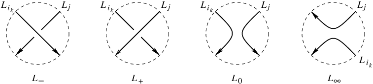
Tree invariants satisfy the following skein relations. Let , , and be four tangles which differ only in the neighborhood of a single crossing , where they look as shown in Figure 11. In other words, has a positive crossing, has a negative crossing, is obtained from by smoothing, and is obtained from by the reflection of orientation of , followed by smoothing. Orders of strings of , and coincide in the beginning of each string. See Figures 11 and 12. We will call , and a skein quadruple.
Theorem 4.3.
Let and . Let , , and be a skein quadruple of tangles on strings which differ only in the neighborhood of a single crossing of -th and -th components, see Figure 11. For denote , . Then
| (7) |
| (8) |
Here we used the notation to stress that .
Remark 4.4.
Example 4.5.

Proof.
To prove Theorem 4.3 consider Gauss diagrams of , in a neighborhood of the arrow corresponding to the crossing of , see Figure 13a.

Here if passes under in the crossing of , and otherwise. There is an obvious bijective correspondence between tree subdiagrams of and which do not include , so these subdiagrams cancel out in pairs in . Since we count only trees with the root on -th string, the only subdiagrams which contribute to are subdiagrams of which contain if , and subdiagrams of which contain if . Note that in each case the arrow is counted with the positive sign (since if , it appears in ). Without loss of generality we may assume that . Thus,
where denote the sum of all maps such that . See the left hand side of Figure 14.

Interpreting and in terms of Gauss diagrams as shown in Figure 13b, and using Proposition 4.2, we immediately get equality (7). See the top row of Figure 14.
Subdiagrams which appear in the equality (8) are shown in the bottom row of Figure 14. To establish (8), it remains to understand why subdiagrams which contain arrows with arrowheads on under cancel out in . Fix and let and be two tree arrow diagrams together with maps , . Suppose that one of the subdiagrams and of contains an arrow, which ends on -th string under . Denote by the lowest such arrow in (as we follow -th string along the orientation). Without loss of generality, we may assume that it belongs to . See Figure 15.

Since ends on the common part of the trunks of and , we may rearrange pieces of to get two different tree diagrams with the same set of arrows as . Namely, removal of from splits it into two connected components and , so that contains strings and contains strings for some . Then is a tree subdiagram of (with trunk on and leaves on ), and is a tree subdiagram of (with the trunk on and leaves on ). See Figure 15. Their contribution to cancels out with that of and to . Indeed, while contain the same set of arrows as , the arrow is now right-pointing, so it is counted with additional factor of . This completes the proof of the theorem. ∎
4.3. Identification with Milnor’s -invariants
It turns out, that for , the tree invariant coincides with a Milnor’s -invariant:
Theorem 4.6.
Let be an ordered (classical or virtual) tangle on strings and let . Then
Proof.
Theorem 3.1 of [8] (together with Remark 2.2) implies that satisfies the same skein relation as (7), that is
Moreover, these invariants have the same normalization for any tangle with the -th string passing in front of all other strings. The skein relation and the normalization completely determines the invariant. ∎
Example 4.8.
Remark 4.9.
Note that in the proof of Theorem 3.3 we did not use the realizability of Gauss diagrams in our verification of invariance of tree invariants under Reidemeister moves in Figure 5, so Theorems 3.3 and 4.6 hold for virtual tangles as well. Recall, however, that in the virtual case there is an alternative definition of ”lower” -invariants of virtual tangles via the lower tangle group, see Section 2.4. To recover these invariants using Gauss diagram formulas we simply reverse directions of all arrows in the definition of the set of tree diagrams .
5. Operadic structure of the invariants
5.1. Tree tangles
Definition 5.1.
A tree tangle is a -tangle without closed components. The string ending on the bottom (that is, on ) is called the trunk of .
We will assume that tree tangles are oriented in such a way that the trunk starts at the top and ends on the bottom of . To simplify the notation, for a tree tangle with the trunk on the -th string we will denote by . There is a natural way to associate to a -tangle with a distinguished string a tree tangle by pulling up all but one of its strings. Namely, suppose that the -th string of a -tangle starts at the top and ends on the bottom. Then can be made into a tree -tangle with the trunk on -th string by the operation of capping shown in Figure 16.

Gauss diagrams of and are the same (since crossings of are the same as in ), so their tree invariants coincide: .
5.2. Operadic structure on tree tangles
Denote by the set of tree tangles on strings. Tree tangles form an operad . The operadic composition
is defined as follows. A partial composition corresponds to taking the satellite of the -th component of a tangle:
Definition 5.2.
Let and be tree tangles, and let . Define the satellite tangle as follows. Cut out of a tubular neighborhood of the -th string of . Glue back into a copy of a cylinder which contains , identifying the boundary with the boundary of in using the zero framing22 2 In fact, the result does not depend on the framing since only one component of ends on the bottom of the cylinder. of . See Figure 17. Reorder components of the resulting tree tangle appropriately.

Now, given a tangle and a collection of tree tangles ,…, , we define the composite tangle by taking the relevant satellites of all components of (and reordering the components of the resulting tangle appropriately).
The following theorem follows directly from the definition of the operadic structure on and the construction of the map from tangles to diassociative trees given by equation (3), Section 3.3.
Theorem 5.3.
The map is a morphism of operads.
References
- [1] S.Chmutov, S.Duzhin, J.Mostovoy. Introduction to Vassiliev knot invariants. Draft, September 9, 2010, 514pp, http://www.pdmi.ras.ru/duzhin/papers/cdbook/
- [2] M. Goussarov, M. Polyak, O. Viro, Finite type invariants of virtual and classical knots, Topology 39 (2000), 1045–1068.
- [3] N. Habegger, X.-S. Lin, The classification of links up to link-homotopy, J. Amer. Math. Soc. 3 (1990), 389–419.
- [4] L. Kauffman, Virtual knot theory, European J. Combin. 20 (1999), no. 7, 663–690.
- [5] J. Levine, The -invariants of based links, In: Differential Topology, Proc. Siegen 1987 (ed. U.Koschorke), Lect. Notes 1350, Springer-Verlag, 87–103.
- [6] J.-L. Loday, Dialgebras, In: Dialgebras and related operads, 7–66, Lecture Notes in Math., 1763, Springer, Berlin, 2001.
- [7] J. Milnor, Link groups, Annals of Math. 59 (1954), 177–195; Isotopy of links, Algebraic geometry and topology, A symposium in honor of S.Lefshetz, Princeton Univ. Press (1957).
- [8] M. Polyak, Skein relations for Milnor’s -invariants, Alg. Geom. Topology 5 (2005), 1471–1479.
- [9] M. Polyak, Minimal generating sets of Reidemeister moves, Quantum Topology 1 (2010), 399–411.
- [10] M. Polyak, O. Viro, Gauss diagram formulas for Vassiliev invariants, Int. Math. Res. Notices 11 (1994), 445–454.