ISW-LSS cross-correlation in coupled Dark Energy models with massive neutrinos
Abstract
We provide an exhaustive analysis of the Integrated Sach–Wolfe effect (ISW) in the context of coupled Dark Energy cosmologies where a component of massive neutrinos is also present. We focus on the effects of both the coupling between Dark Matter and Dark Energy and of the neutrino mass on the cross-correlation between galaxy/quasar distributions and ISW effect. We provide a simple expression to appropriately rescale the galaxy bias when comparing different cosmologies. Theoretical predictions of the cross–correlation function are then compared with observational data. We find that, while it is not possible to distinguish among the models at low redshifts, discrepancies between coupled models and CDM increase with . In spite of this, current data alone seems not able to distinguish between coupled models and CDM. However, we show that upcoming galaxy surveys will permit tomographic analysis which allow to better discriminate among the models. We discuss the effects on cross-correlation measurements of ignoring galaxy bias evolution, , and magnification bias correction and provide fitting formulae for for the cosmologies considered. We compare three different tomographic schemes and investigate how the expected signal to noise ratio, , of the ISW–LSS cross–correlation changes when increasing the number of tomographic bins. The dependence of on the area of the survey and the survey shot noise is also discussed.
Subject headings
(cosmology:) cosmic microwave background; cosmology: miscellaneous; cosmology: observations; cosmology: theory; cosmology: large-scale structure of universeI. Introduction
Several observations made over the recent years, related to a large extension to Large Scale Structures (LSS) and anisotropies of the Cosmic Microwave Background (CMB) as well as the magnitude–redshift relation for type Ia Supernovae have given us a convincing picture of the energy and matter density in the Universe [70, 75, 82, 83, 39].
Baryonic matter accounts for no more than 30 of the mass in galaxy clusters while the existence of a large clustered component of Dark Matter (DM) seems now firmly established, although its nature is still unknown. However, they contribute to the total energy density of the Universe with only a few percent and about 25 respectively.
No more than another few percent could be accounted for by massive neutrinos, but only in the most favorable, but unlikely case. According to Kristiansen et al [37] (see also Elgarøy et al [21]) the total mass of neutrinos cannot exceed the limit of 1.43 (see, however, La Vacca et al [40], La Vacca et al [42], Kristiansen et al [38] for a recent analysis on neutrino mass limits in coupled dark energy models). A very small part of the total energy density is due to massless neutrinos and CMB radiation.
The model suggested by observations is only viable if the remaining 75 is ascribed to the so–called Dark Energy (DE) responsible for the present day cosmic acceleration.
Although strongly indicated by the observations, the existence of DE is even more puzzling than DM. It can be identified with a cosmological constant or with a yet unknown dynamical component with negative pressure. On the other hand, its manifestation can be interpreted as a geometrical property of the gravity on large scales resulting from a failure of General Relativity (GR) on those scales (see Copeland et al [17] for a review).
Within the context of GR, as an alternative to the cosmological constant, DE is usually described as a scalar field , self–interacting through a suitable potential , or a cosmic fluid with negative pressure Peebles & Ratra [68] (see Koivisto & Mota [35], Koivisto, Mota & Pitrou [36], Li, Barrow & Mota [45] for alternatives and references therein).
Scalar fields naturally arise in particle physics. Furthermore, if they are tracker fields [77], fine tunings associated to the small value of the present DE energy density can be significantly alleviated unlike the cosmological constant case.
In addition to self–interaction, a scalar field can in principle be coupled to any other field present in nature. However, in order to drive the cosmic acceleration, its present time mass is expected to be, at least on large scales, ( being the present Hubble parameter). Such a tiny mass gives rise to long–range interactions which could be tested with fifth–force type experiments. Couplings to ordinary particles are strongly constrained by such a kind of experiments but limits on the DM coupling are looser (constraints on coupling for specific models were obtained in Maccio’ et al [49], Amendola & Quercellini [4], Olivares et al [65], Lee et al [43], Guo et al [27], Mainini & Bonometto [50] from CMB, N-body simulations and matter power spectrum analysis).
A possible common origin of DM and DE and/or a their direct coupling [86, 2, 23, 7, 16, 76, 22]. would ease one of the most critical problems in modern cosmology, the so–called coincidence problem: why expansion started to accelerate just at the eve of our cosmic epoch, after decelerating during all epochs after inflation? Why DE and DM have similar densities just now? Because of the coupling DM and DE densities keep similar values during a long period and the only peculiar feature of the present epoch is the recent overtaking of DM density by DE density.
If present, DM–DE coupling could have a relevant role in the cosmological evolution affecting not only the overall cosmic expansion but also modifying the DM particles dynamics with relevant consequences on the growth of the matter density perturbations in both linear and nonlinear regime (e.g., on halo density profiles, cluster mass function and its evolution, see Wang & Steinhardt [85], Mainini et al [51], Mainini et al [52], Klypin et al [33], Dolag et al [19], Maccio’ et al [49], Perrotta et al [71], Mota & Barrow [58], Olivares et al [66], Nunes et al [63], Mota & van de Bruck [59], Maor & Lahav [56], Nunes et al [63], Wang [84], Manera & Mota [55], Nunes & Mota [64], Dutta & Maor [20], Mota et al [60], Mainini [53], Shaw & Mota [81], Mota [57], Mainini [54], Baldi et al [5], Wintergest & Pettorino [87], Baldi & Pettorino [6]. LSS is then a powerful probe of DE nature which permit to put significant constraints on DE parameters. Constraints often become even more stringent when data from other probes are simultaneously taken into account.
CMB is another powerful probe of DE nature. In principle, by joining anisotropy and polarization data, DE parameters can be significantly constrained. CMB and LSS probe the universe at different epochs and are therefore complementary to each other. Future data from high resolution CMB experiment like PLANCK 11 1 http://www.rssd.esa.int/index.php?project=planck and LSS surveys (EUCLID 22 2 http://www.euclid-imaging.net/, LSST 33 3 http://www.lsst.org/lsst, DES 44 4 https://www.darkenergysurvey.org/, JDEM 55 5 http://jdem.gsfc.nasa.gov/, etc) will allow to constrain DE up to an unprecedented accuracy.
In this paper we will focus on the Integrated Sachs Wolfe (ISW) effect [78]. ISW effect is a secondary anisotropy of the CMB and a direct signature of DE. The effect arises when a photon from the last scattering surface passes through a time–dependent gravitational potential changing its energy so that additional temperature anisotropies are generated. Decay of gravitational potentials may occur through cosmic curvature, in the presence of DE or in alternative gravity models.
Assuming General Relativity is the correct theory of gravity and that the Universe is spatially flat, large–scale gravitational potentials do not evolve significantly in the matter era. Cosmic acceleration, however, causes the gravitational potentials to decay making the ISW effect highly sensitive to the presence of DE.
Though difficult to detect directly in the CMB, ISW signal can be measured by cross–correlating the CMB with tracers of LSS and has recently been detected using WMAP data of CMB in combination with several LSS surveys at the the confidence level providing independent evidence for the existence of the DE (see Giannantonio et al [25], Xia et al [88] and references therein).
Cross-correlation then provides a powerful method to discriminate among different DE models and, in particular, to detect a possible interaction between DE and DM other than investigate the clustering properties of DE on large scales. If present, DM–DE coupling changes both the scaling of the DM energy density and the growth rate of matter perturbations yielding a significant evolution of the metric potentials even in the matter era.
The aim of this paper is to provide an exhaustive analysis of the ISW effect in the contest of the so called coupled DE cosmologies [3] mainly focusing on the effects of the DM–DE coupling on the cross–correlation between galaxy/quasar distributions and ISW effect.
Such models can be motivated in the contest of scalar–tensor theories of gravity or describe the low energy limit of a more fundamental theory beyond the standard model of particle physics, e.g. string theory.
The models which we aim to investigate differ from the standard CDM in three different aspects: (i) DE is a self–interacting scalar field rather than a cosmological constant . We shall consider a class of self–interaction potentials admitting tracker solutions. (ii) A linear DM–DE coupling is allowed. (iii) We allow neutrinos to be massive.
The effects of massive neutrinos in cosmology have been studied thoroughly for many years (for a review see Lesgourgues & Pastor [44]). Cosmological observations are mostly sensitive to the sum of neutrino masses, . Currently, the strongest upper limit on neutrino mass scale comes from cosmology. One of the effects of massive neutrinos is to induce a small decay of the gravitational potentials during both matter and DE domination so that, in principle, ISW effect would also provide information on their mass. Furthermore, as recently outlined in La Vacca et al [40], La Vacca et al [42], Kristiansen et al [38] the effects that massive neutrinos have on the angular power spectrum of the CMB anisotropies, , and matter power spectrum, , are almost opposite to those of the DM–DE coupling, resulting in a strong degeneracy between the coupling strength and . A recent analysis by means of Monte Carlo Markov Chain method has shown that a cosmology with significant and is statistically preferred to one with no coupling and almost massless neutrinos. Further, when priors on the neutrino mass from earth-based neutrino mass experiments (Heidelberg-Moscow neutrinoless double -decay, KATRIN tritium -decay 66 6 http://www-ik.fzk.de/katrin/publications/documents/Design Report2004-12Jan2005.pdf) are added to the analysis, a detection of a DM-DE coupling is found.
The plan of the paper is as follows: in Section 2 we describe our model while the ISW effect theory is reviewed in Section 3 where we also discuss how the ISW signal depends on the main parameters of the model. In Section 4 we discuss galaxy bias and magnification bias. Comparison between theoretical prediction and observation data is presented in Section 5 while a tomographic analysis is performed in Section 6. Section 7 is devoted to the conclusions.
II. The model
We assume a spatially flat Friedmann–Robertson–Walker (FRW) background with metric ( is the conformal time) filled with baryons, photons, neutrinos, DM and a component of DE which will be ascribed to a scalar field self–interacting through a potential . In the following, the indexes , , and will denote baryons, cold DM, massive neutrinos and DE. Photons and massless neutrinos will be referred as radiation and denoted by .
In addition to self–interaction we also consider a possible interaction between the scalar field and DM. Here we give only the equations for baryons, DM and DE being the equations for the other components the usual ones (see, e.g Ma & Bertschinger [48]).
The Friedmann equation for the scale factor , the continuity equations for baryons and DM and the evolution equation for the scalar field read:
| (1) | |||
| (2) | |||
| (3) | |||
| (4) |
where denotes the derivative with respect to , , is the energy density of the component and the constant parametrizes the DM–DE coupling strength.
Working in the conformal Newtonian gauge the metric of a perturbed flat FRW Universe takes the form:
| (5) |
where plays the role of the Newtonian potential, is the Newtonian spatial curvature, and:
| (6) | |||
| (7) |
where , , , and are the density parameter, density contrast, four–velocity divergence, shear and state parameter of the component ( and being the pressure of the component and the critical density of the Universe).
Linear perturbation equations for DM and baryons read:
| (8) | |||
| (9) | |||
| (10) | |||
| (11) |
where is the baryon sound speed, is the standard term describing momentum exchange with photons due to Thomson scattering (see, e.g Ma & Bertschinger 1995) and is the perturbation to the scalar field which evolves according to:
| (12) |
As we are interested in the cross–correlation between ISW effect and galaxy distributions, above equations can be simplified. At late time radiation and massive neutrinos can be neglected so that no shear stresses are present and . Furthermore, the cross–correlation signal comes from scales well within the horizon, Mpc, so that the second term in (6) can be neglected.
The above equations then reduce to the usual Poisson equation for the gravitation potential:
| (13) |
a modified Jeans equation for DM and the usual one for baryons:
| (14) |
and a Poisson–like equation for the scalar field perturbation:
| (15) |
where we have defined the dimensionless coupling parameter:
( is the Planck mass).
As clearly visible from the above equations and widely discussed in Amendola [3], coupling affects the dynamics of DM particles. As a consequence baryons and DM develop a bias , i.e. . Notice that, this bias, which origin is to ascribe to the coupling, is something completely different from the galaxy bias due to hydrodynamical effects, discussed in the subsequent sections.
It is also worth mentioning that, unlike the uncoupled case, in the presence of coupling, Universe goes through an evolutionary phase named –matter dominated era (MDE) just after matter–radiation equivalence. In this period the scalar field behaves as () having a non–negligible kinetic energy which dominates over the potential one. After this stage, the usual matter era follows before entering in the accelerated regime with a final De Sitter attractor. Notice also that, because of the MDE and the non–usual scaling of the DM energy density, i.e. , after equivalence the background expansion law will differ from the usual .
II.1. Potential


We shall consider the Ratra–Peebles (RP) [74] and SUGRA self–interaction potentials [12], reading
and
respectively; they allow tracker solutions for any . For both potentials, once and are assigned, the present time DE density parameter is uniquely defined.
Limits on these models without coupling between DE and CDM have been studied in La Vacca & Kristiansen 2009. They find, that only quite small are allowed. In the SUGRA case in particular only is allowed. Such small values are well below the range motivated by particle physics. Therefore the physical appeal of the SUGRA potential is spoiled.
Let us however outline that, when the degree of freedom is opened, values as large as 30 GeV become allowed, at the 1-- level, while, at the 2– level, no significant constraint on the energy scale remains. Even for the RP potential, for which a limit held, in the absence of coupling, values become allowed (La Vacca et al 2009).
In the absence of DM–DE coupling, RP yields quite a slowly varying state parameter. On the contrary, SUGRA yields a fast varying . Although coupling causes a behavior significantly different from the uncoupled case, one could again consider these potentials as examples of rapidly or slowly varying .
The results shown in the next two sections are qualitatively the same for RP and SUGRA models. We will show them only for SUGRA cosmologies while the results for RP models will be shown only when comparing the theoretical predictions with observational data and dealing with redshift tomography.
III. ISW effect
ISW effect arises when CMB photons from the last scattering surface pass through a time–dependent gravitational potential changing its energy so that additional temperature anisotropies are generated. The ISW temperature fluctuation, , is given by:
| (16) |
where is the CMB temperature and is the visibility function of the photons.
As outlined in previous section, we will deal with scales within the horizon and redshifts such that radiation and any anisotropic stress can be neglected () . In the matter era and in the absence of DM–DE coupling (), Poisson equation reads:
| (17) |
( and are the total matter density parameter and density contrast respectively) from which one can appreciate that the gravitational potential stays constant, , and no ISW effect arises. However, when DE starts to dominate the cosmic expansion, is no longer constant and ISW effect generates secondary anisotropies in the CMB.
On the other hand, as explained in the previous section, DM-DE coupling affects both the background and density perturbation evolution, resulting in a variation of even during the matter domination.
Figure 1 shows how and affect the time evolution of the sum which time derivative forms the source of the ISW effect. Evolution of the gravitational potentials is obtained by a modified version of the public code CMBFAST integrating the fully relativistic equations and taking into account the contributions of all of the components, i.e, photons, DM, baryons, neutrinos and DE.
Notice how and affect in an opposite fashion.
Performing a measurement of the ISW effect is, however, a difficult task because of its small signal compared with that of primary anisotropies ( times larger). Furthermore, while on small scales the small differences in temperature tend to cancel out, the large scales, from which the most ISW effect contributes come from, are strongly affected by the cosmic variance.
The problem can be overcome by cross–correlating the ISW anisotropies with some tracers of the matter density, e.g. astrophysical objects like galaxies.
The observed galaxy density contrast in the direction is:
| (18) |
where is the normalized selection function of the galaxy survey and is the galaxy bias, which will be discussed in the next section, relating the galaxy density contrast to the inhomogeneities in the mass distribution, . Since is related to the gravitational potential through the Poisson equation, the observed galaxy density will be correlated with the ISW anisotropies in the nearby direction :
| (19) |
The 2–point angular cross–correlation function (CCF) and auto–correlation function (ACF) in the harmonic space are then defined as:
| (20) | |||||
where , ’s are the Legendre polynomials and the cross– and auto–correlation power spectra are given by:
| (21) |
where is the primordial power spectrum of scalar perturbations and the integrands and are:
| (22) | |||
| (23) |
(here are the spherical Bessel functions, and is the comoving distance).

In the following we use our modified CMBFAST code to calculate the theoretical CCF and ACF. In order to better understand the effects of , and on them, we start to compute the ISW-matter CCF and ACF, and , and power spectra, and , the values of which are obtained similar to (20) and (21) by replacing and with:
| (24) | |||
| (25) |
where the only difference from and is the bias factor. Here, we model as a narrow Gaussian centered at two different redshifts, z=0.3 and z=3. This will permit to obtain some information about the time evolution of the correlations. Realistic selection functions will be considered in the next sections. Cosmological parameters are assumed to be the same as in the WMAP 5 years best fit CDM model [34].
III.1. Dependence on , and
Let us consider first the uncoupled case () and no massive neutrinos. Figure 2 shows the redshift evolution of the gravitational potentials (left panel) and the source of ISW effect (right panel) for different values of . The dependence on of the ISW-matter correlations and is then displayed in Fig. 3 at two different redshifts, and . When increasing , both and show an opposite behavior at low and high redshifts. This reflects the behavior of .
In the presence of coupling one can distinguish between two different behaviors for small and large ’s. This is shown in Figs. 4 and 5 for . In the first case, the evolution of the gravitational potentials and the cross–correlation signal are almost independent from . It can be understood noticing that for small , MDE is very long and the usual tracker solution is (almost) never reached. In this phase, coupling terms in the field equations dominate so that the tracker solution is almost independent from . When increasing , MDE becomes shorter and the behavior resemble that of the uncoupled case. The transition between the two above regimes occurs around GeV.
Dependence on is shown in Figs 6 and 7. Again, the behavior of the cross–correlation reflects that of the ISW source. However, while coupling can have opposite effects on the cross-correlation at different redshifts, i.e. it can increase or decrease the signal, massive neutrinos always decrease the signal. It is shown in Fig. 8 which displays the behavior of as a function of at two different redshifts. Cross-correlation signal always decreases at the increasing of the neutrino mass.
IV. Galaxy bias and magnification bias
The galaxy bias can, in general, evolve both in redshift or as a function of the scale. However, on the large scales of interest for the ISW effect, the bias is usually assumed to be linear, spatially constant and only redshift–dependent, i.e. . This assumption is fully consistent with results from numerical simulations, redshift surveys and semi–analytic calculation in the contest of the so–called halo–model (see [9, 69]).
However, given a galaxy selection function picked at certain redshift , the bias can be approximated with an appropriated constant. In this case it will be
| (26) |
Within the above approximation, given a particular survey and assumed a cosmological model, the bias is usually estimated by fitting the theoretical matter–matter correlation function, , for the assumed cosmology, to the observed galaxy–galaxy correlation function, .
Biases have been estimated for different surveys by several authors assuming the WMAP best fit CDM cosmology (see Boughn & Critteden [11], Boughn & Critteden [10], Giannantonio et al [24], Myers et al [61], Rassat et al [73], Blake et al [8]). Since we are considering cosmological models different from a CDM, we need to appropriately rescale those biases to each of the our models. Note, however, how the estimation of in (26) depends on the normalization of the power spectrum in (see (21)). For a fixed normalization, taking into account (26), biases will be rescaled according to:
| (27) |
where indicates the average on the angular scales of interest.
However, (27) should be generalized when magnification bias effect due to gravitational lensing is non–negligible. Gravitational lensing by intervening matter changes the observed galaxy number density , leading a correction term being added to the intrinsic galaxy fluctuation
With this correction, the observed ACF becomes:
| (28) | |||||
where and the rescaled bias will then be the solution of:
| (29) |
Auto– and cross–correlations corrected for magnification bias are obtained considering in (25) the function [29]:
| (30) |
where is the slope of the number counts of galaxy number density as a function of the flux, . It depends on the choice of galaxy sample and is redshift dependent. The lensing window function (in a flat Universe) is:
Magnification bias increases with redshift and could be important when dealing with deep survey, e.g. quasars. This is shown in Fig. 9 which compares the effect of the magnification bias on the ISW-gal correlation at and . A detailed analysis on how magnification bias affects ACF and CCF can be found in LoVerde et al [46], Hui et al [31], LoVerde et al [47], Hui et al [32].


| Parameter | RP | SUGRA |
|---|---|---|
| 2.260 0.061 | 2.260 0.065 | |
| 0.1039 0.0062 | 0.1042 0.0084 | |
| 0.087 0.016 | 0.088 0.017 | |
| (eV) (95% C.L.) | 1.13 | 1.17 |
| (95% C.L.) | 0.17 | 0.18 |
| -4.2 | 6.3 | |
| 0.969 0.015 | 0.970 0.018 | |
| ln | 3.055 0.040 | 3.057 0.041 |
| (km/s/Mpc) | 71.8 2.5 | 71.9 2.7 |
| CDM | RP | SUGRA | |
|---|---|---|---|
| 2MASS | 1.40 | 1.46 | 1.47 |
| SDSS gal | 1.00 | 1.03 | 1.04 |
| LRG | 1.80 | 1.83 | 1.84 |
| NVSS | 1.50 | 1.53 | 1.54 |
| HEAO | 1.06 | 1.09 | 1.09 |
| QSO | 2.30 | 2.33 | 2.33 |


.

V. Comparison to observational data
Investigations of CMB–LSS correlations were made in a recent series of works which rely on
WMAP data and a variety of LSS probes [62, 1, 13, 14, 73, 72, 29, 25, 88].
There is an overall agreement among different groups in finding an evidence for a positive ISW effect at the confidence level. It was also found a substantial agreement between the observed cross-correlations and the expected signal arising from the ISW effect in the WMAP best fit CDM cosmology. Different DE mod
els were also considered in Olivares et al [67], Schäfer [79], Giannantonio et al [26].
In a recent work [25] a combined analysis of the ISW effect was performed by cross–correlating CMB map provided by the WMAP collaboration with all the relevant large scale data sets and modeling their covariance properties with different methods.
In this section, we compare our theoretical predictions based on the models described above with the measurements made in Giannantonio et al [25] by considering six different galaxy catalogues: the optical Sloan Digital Sky Survey (SDSS), the infrared 2 Micron All-Sky Survey (2MASS), the X-ray catalogue from the High Energy Astrophysical Observatory (HEAO) and the radio galaxy catalogue from the NRAO VLA Sky Survey (NVSS). In addition, given the high quality of the SDSS data, some further subsamples was extracted from it, consisting of Luminous Red Galaxies (LRG) and quasars (QSO).


As shown in Fig. 10 their redshift distributions, , span a redshift range . In order of increasing mean redshift of the sample we have: 2MASS, SDSS galaxies, LRG, NVSS, HEAO and QSO (for details on the catalogues see Giannantonio et al [25], Ho et al [29].
Constraints from CMB, SNIa and LSS on cosmologies with coupling and massive neutrinos have been obtained in La Vacca et al [42], Kristiansen et al [38] by means of Monte Carlo Markov Chain technique. Best fit parameters from their analysis will be used in this and in the next section when dealing with redshift tomography. Parameters are summarized in Table 1 where are the physical baryon and cold dark matter density parameters, , where is the dimensionless Hubble parameter, is the optical depth to reionization, is the scalar spectral index, denotes the amplitude of the scalar fluctuations at a scale of , , assuming 3 equal neutrino masses , denotes the energy scale in DE potentials, while is the coupling parameter between DM and DE. In the following we will use and for RP and SUGRA respectively which correspond to the For the three splitting schemes described above 1– limits. Best fit parameters for coupling and neutrino mass are approximately the same for both model, i.e. and .
For each catalogue and model, biases are shown in Table 1 and calculated according to (27) using for the values given in Giannantonio et al [25]. Given the low mean redshifts of the catalogues we neglect the magnification bias effect which amounts to a few percent only in the case of quasars. It will be, however, considered in the next Section when dealing with redshift tomography and higher . We will also discuss how good to approximate with a constat is.
For each catalogue, we then determine the expected CCFs for our models.
Comparison with observational data is shown in Fig. 11 for SUGRA and RP models. The predictions for the CDM is also displayed. Note that, because of know contamination from Sunyaev–Zeldovich effect in the 2MASS data [41], the four smallest angle bins should be disregarded. While it is not possible to distinguish among the models at low redshifts, discrepancies between coupled models and CDM increase with even though RP and SUGRA models remain indistinguishable. In spite of this, however, current data alone seem not able to discriminate between coupled models and CDM.
VI. Redshift tomography
As already outlined, unlike uncoupled DE models with massless neutrinos, both coupling and massive neutrinos causes the gravitational potentials to evolve even in the matter dominated epoch. Therefore, a detection of a non–vanishing ISW effect signal at such high redshifts would rule out a vast class of DE models indicating a possible interaction in the dark sector. Upcoming galaxy surveys will cover a large redshift range. One goal will be to use the photometric redshifts of the galaxies to split the survey into multiple redshift bins allowing for tomographic analysis.
Following the procedure of Hu & Scranton [30], given a galaxy distribution, , the galaxies can be divided into photometric bins, labelled with index :
Assuming a distribution of the standard form:
| (31) |
and that the photometric redshift errors are Gaussian distributed with an rms fluctuation , the resulting photometric redshift distributions are given by:
We now propose to study how a tomographic analysis is affected when considering different splitting schemes. This will permit to single out the optimal splitting choices which guarantee a signal to noise ratio, , high enough to distinguish among different DE models.
As we are interested in high , we model the overall distribution according to (31) with , and . These values provide a good fit of the quasar distribution from SDSS DR6 considered in the previous section [88]. We assume the shape of such a distribution to be approximately the same as for that expected from future surveys.
| quasar bias | magnification bias | snr |
|---|---|---|
| no | 4.56 | |
| no | 4.31 | |
| yes | 4.61 | |
| yes | 4.38 |
| quasar bias | magnification bias | |
|---|---|---|
| a) | no | |
| b) | no | |
| c) | yes | |
| d) | yes | |
| e) | yes |


Further, we assume as expected from future experiments, and consider three different splitting schemes, each with bins in the redshift range from to :
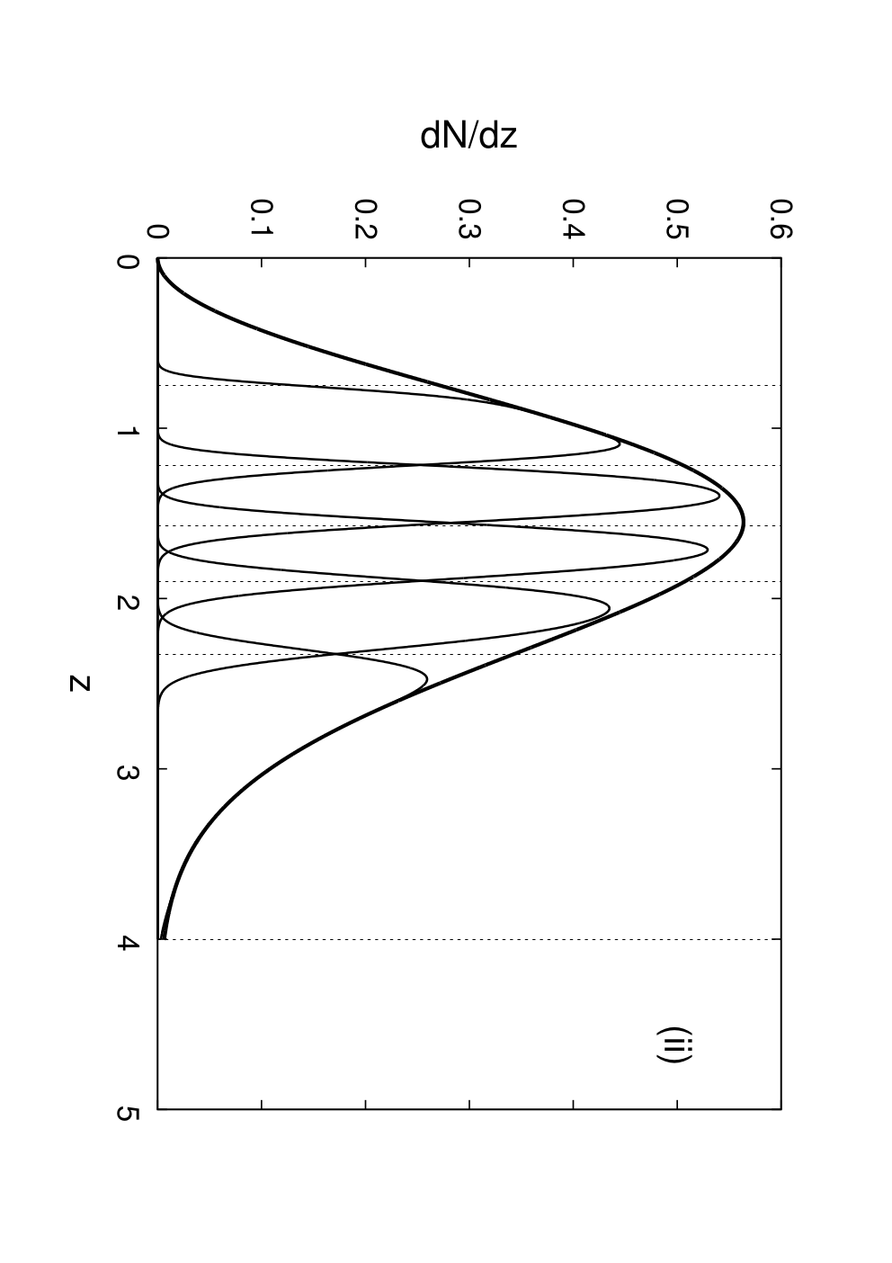
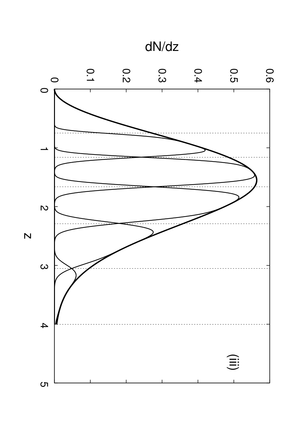
(i) bins equally spaced in , with ;
(ii) same number of galaxies, , in each bin;
(iii) bin sizes increasing proportionally to the photometric error, .
The three splitting schemes are shown in Fig. 12. The thick line is the overall quasar distribution while the other curves are the true (spectroscopic) distributions that correspond to the divisions (vertical lines) in photo-z space.
We also take into account magnification bias effect which can be important at higher . In a recent analysis by Ho et al [29], the slope of the quasar counts, , entering in (30), was found to be redshift dependent. They found in the photometric redshift range and for . For simplicity, we assume a constant slope as in Xia et al [88].
VI.1. Dependence on galaxy bias evolution and magnification bias
Before comparing the different models we discuss the effects of ignoring magnification bias and quasar bias evolution. This is done for the CDM cosmology. Results, however, are valid for RP and SUGRA as well.
Notice that implications of galaxy bias evolution on ISW measurements and parameter estimation has been considered in a pioneer work of Schaefer et al 2009.
For the quasar bias evolution in CDM, we use the empirical formula derived by Croom et al [18]:
| (32) |
which provides a good fit of the recent observational findings by Xia et al [88].
We first consider the overall quasar distribution and calculate the expected signal–to–noise ratio, snr, of the cross–correlation in the following cases: constant quasar bias (where is the mean redshift of the survey) and as given by (32). For each of them, the snr is obtain by neglecting or considering the magnification bias correction. Results are summarized in table 4.
For Gaussian fileds, the expected is given by (see e.g. [15]):
| (33) |
where is the noise contribution to the ISW ( and being the total anisotropy contribution and any detector noise contribution, negligible on the scales we are interested in) while , is the shot noise associated with the galaxy/quasar catalog ( is the surface density of galaxies/quasars per steradians). is the fraction of sky common to CMB and galaxy/quasar survey maps.
Note that (33) is strictly true only in the case of Gaussian fields and full–sky coverage, . In this section, we assume that to be the case other than a negligible . These assumptions will be relaxed in the following. Anyway, for partial sky coverage, one can, in first approximation, multiply for the values of here presented.
The value of the lowest multipole, , can be approximately set to in order to account for the loss of low multipole modes. Anyway, although a significant part of the ISW signal comes from lower multipoles, we set in order to avoid effects of gauge correction on very large scales recently discussed by [90] even if this implies a reduction of . The maximum multipole, , is set to . However, we will show later that the contribution to from multipoles is negligible.
From Table 4, it follows that cross–correlation measurements are more affected by errors when ignoring the quasar bias evolution rather than the magnification bias correction. In fact, in this last case, an error of on snr is obtained while in this last case while the error raises to if the quasar bias is approximated by a constat value, ( being the mean redshift of the quasar distribution) and it is of if both quasar bias evolution and magnification bias are neglected.
We now turn to tomography. According to (33), the signal to noise ratios, , in the i–th tomographic bin are calculated for each of the cases listed in Table 4. Fig. 13 shows the errors relative to the case for each bin of the three splitting schemes described above. Unlike the overall quasar distribution, in each bin, distributions are very narrow and the quasar bias can be approximated by a constant, ( being the mean redshift of the –th bin), leading to only a minor error on (case ). On the other hand, ignoring magnification bias correction might be critical at high (, case ) and if a constant bias, , is used for all bins, the error can reach at higher redshifts.


However, since photometric redshift errors cause the bins to overlap and magnification of the galaxies at probes structures at , cross–correlation measurements at high are quite correlated with those at low redshifts. Taking into account such correlations, the net accumulated for measurements from all the bins up to is given by:
| (34) |
| (35) |
The relative error on is shown in Fig. 14 for the same cases as in Fig. 13. In all cases, despite the significant differences in in high bins, errors are always . This is understood because most of the cumulative snr comes from low redshifts. However, in the case , errors considerably increase if the shot noise associated to the catalog is non–negligible. Fig. 15 compares the relative errors on (top panel) and (bottom panel) in the case of negligible shot noise and assuming a SDSS DR6–like survey with a number density of quasars, , of . In this last case, the error on the cumulative ranges from , to , depending on the number of bins considered while the error on can also reach the in bins at higher redshift.
VI.2. Model comparison
In the previous section we have shown that when dealing with narrow tomographic bins, we can approximate the galaxy bias in each bin with a constant committing an error of no more than a few percent.
Then, after calculating the cross–correlation power spectra for the best fit CDM, SUGRA and RP models we apply (29) to each bin of the three splitting schemes. The rescaled biases and are then fitted with an expression similar to (32) obtaining:
for RP and
for SUGRA. These expressions, which will be used in the rest of the paper, are valid up to leading a galaxy bias evolution only slightly different from that of CDM.
In Fig. 16, we show the cross–correlation power spectra for the splitting (i). Lower frames of each panel display the ratio between the SUGRA and RP spectra and the CDM spectrum. Mean redshifts of the true bin distributions are also indicated. A similar redshift evolution could be obtained by considering (ii) or (iii). As clearly visible from the figure, a better discrimination among the models is expected at higher redshifts.
The expected and for the different splitting schemes are shown in Figs. 17 and 18 respectively, for the cosmologies considered. Despite the same qualitative behavior for all the models, higher are expected in the SUGRA case; RP being in the between of SUGRA and CDM. Horizontal lines in Fig. 18 indicate the obtained by using the full distribution.
For each splitting scheme, in Figs. 19, we plot the ratio between the RP and SUGRA and values and those expected in the CDM case. A first thing to note is the overlapping, for both RP and SUGRA, of the three curves corresponding to the different splittings indicating that the three schemes considered perform equally well in discriminating among the models. A better discrimination is however achieved looking at high redshifts.
In Fig. 20, we investigate how changes when increasing the number of the bins (left panel) and whether a greater number of bins could permit to better discriminate between models (right panel). Results are shown for the splitting scheme (iii) with 2,3,5,10 bins in the RP model. Similar results are obtained in the other cases. in the case of no splitting is also shown. More bins, in principle, would permit to have a more detailed description of the redshift evolution of ISW effect. However, as clearly visible in the left panel, the decreases at the increasing of the bin number. In the right panel, RP model is compared to CDM. Even though, at high redshifts, tomography permits to distinguish among the models better than using the full distribution, the figure shows that increasing the number of the bins from 2 to 10 would permit only a minor improvement in discriminating between the models.
VI.3. Sky coverage and shot noise
Up to now, we have considered the ideal case of Gaussian fields, full sky coverage and negligible shot noise. However, after cutting out our galaxy from the analysis, future CMB and galaxy maps are expected to cover, at best, a sky fraction . In this case different multipoles are no longer independent and (33), (34) and (35) only provide approximated estimations and a more rigorous analysis taking into account for the effective survey geometry is needed ([14], [28], [89]). It has been however shown that, under the above approximations, a better estimation can be obtained by binning the power spectra data in bins of appropriate size making the bins independent. In this case, (33) and (34) are increased by a multiplicative factor of . [14] found that works well for .
In Figs. 21 and 22 we show some results for the cumulative from all the bins of the splitting (iii). Results are however the same for the other schemes.
The left panel of Fig. 21 shows the contribution to the cumulative from each multipole while the cumulative up to is displayed in the right panel. The dependence on and has been removed. As clearly visible, most of the cross-correlation signal comes from lower multipoles and contributions from are negligible.
In Fig. 22 cumulative contour levels are plotted in the plane where is the quasar number density for a SDSS DR6-like survey. Given that such a survey cover of the sky, future experiments covering a sky fraction will increase the cumulative of a factor if the shot noise is reduced by and a factor in the case . No significant improvement is obtained by further reducing the shot noise. For and negligible shot noise, the increasing of in the –th tomographic bin can range from a factor of (low bins) up to (high bins). This is shown in Fig. 23.
VII. Conclusions
In this work we have investigated ISW-LSS cross-correlation in coupled Dark Energy models with massive neutrinos. The presence of a coupling between DM and DE as well as massive neutrinos change both the background and matter perturbation evolutions yielding, unlike the CDM case, a time–variation of the gravitational potentials even during the matter domination. A significant ISW signal is thus expected also at high redshifts.
Firstly, we have investigated the dependence on the energetic scale, , of the DE potential, the coupling strength and the neutrino mass . We considered first the uncoupled case () and massless neutrinos. We found that, when increasing , both and show an opposite behavior at low and high redshifts. This in fact reflects the behavior of . In the presence of coupling one can distinguish between two different behaviors for small and large ’s. In the first case, the evolution of the gravitational potentials and the cross–correlation signal are almost independent from . It can be understood noticing that for small , coupling terms in the DE field equations dominate so that its solution is almost independent from . When increasing , the behavior resemble that of the uncoupled case. Dependence on was also investigated and, again, the behavior of the cross–correlation at different redshifts reflects that of the ISW source. However, while coupling can affect (and ) in an opposite fashion at high and low redshifts, massive neutrinos always decrease the cross–correlation signal.
Secondly, we have provided a simple expression, eq. (27), which permits to appropriately rescale the galaxy bias when comparing different cosmologies once the bias of a particular model, e.g. CDM , is known and the normalization of the power spectrum in each model is fixed. We also give, a generalized version of (27) to the case when the magnification bias effect due to gravitational lensing is non–negligible (see eq. (29)).
Then, we compare the theoretical prediction on the cross–correlation function for our models with the observational data obtained for six different galaxy catalogues by Giannantonio et al [25]. We found that, while it is not possible to distinguish among the models at low redshifts, discrepancies between coupled models and CDM increase with even though RP and SUGRA models remain indistinguishable. In spite of this, however, current data alone seem not able to discriminate between coupled models and CDM.
Finally, we studied the redshift tomography. Upcoming galaxy surveys will cover a large redshift range also providing photometric redshifts of the galaxies with high accuracy. This will permit to split a survey into multiple photometric redshift bins allowing for tomographic analysis. Here, we were interested to study how a tomographic analysis of the ISW–LSS cross–correlation is affected when considering different splitting schemes and assuming photometric redshift errors as expected from future experiments. As we were interested in high redshifts, where our models, unlike the CDM case, are expected to provide a significant ISW effect signal, ISW effect was cross–correlated with quasars. The quasar distribution was thus split in tomographic bins according to three different schemes: (i) bins equally spaced in ; (ii) same number of galaxies, in each bin; (iii) bin sizes increasing proportionally to the photometric error. Cross-correlation were then calculated in each bin.
Our tomographic study was based on a signal–to–noise analysis.

We started our discussion investigating the effect on of ignoring the quasar bias evolution and magnification bias correction for an ideal survey. We found that, if the overall quasar distribution is used, cross–correlation measurements are more affected by errors when ignoring the quasar bias evolution () rather than the magnification bias correction ()
However, when dealing with tomography the error on ( indicating the –th bin) never overcome if the quasar bias in each bin is approximated with an appropriated constant, but it can reach , at high redshifts, when magnification bias is ignored. Errors on the cumulative , however, always stay below the . On the other hand errors can increase up to if the shot noise associated to the quasar survey is set to the current values.
We then used the tomographic analysis in order to compare different cosmologies. We found that the above splitting schemes, perform equally well in discriminating among the models. A better discrimination is however achieved looking at high redshifts.
We also investigated how the expected signal to noise ratio, , of the cross–correlation changes when increasing the number of the bins and whether a greater number of bins could permit to better discriminate between models. Even though more bins would allow to have more information on the redshift evolution of the ISW effect, the decreases at the increasing of the bin number. As a consequence, although tomography, at high redshifts, would permit to distinguish among the models better than using the full distribution, when comparing our models to CDM it was shown that increasing the number of the bins from 2 to 10 would permit only a minor improvement in the discrimination.
Finally, we showed that future wide field surveys () can increase the cumulative of the cross–correlation of a factor () if the current shot noise is reduced by () while the of the single bins can increase up to a factor at high redshift.
Our analysis suggest a discrimination power of future ISW–LSS cross-correlation measurements able to distinguish among different cosmologies. However, in order to assess the discrimination, more rigorous analysis in terms of Fisher Matrix and Monte Carlo Markov Chain are needed. They are currently under investigation and left for future works.
Acknowledgments
Tommaso Giannantonio is gratefully thanked for providing observational data on cross–correlation and useful hints. DFM thanks the Research Council of Norway FRINAT grant 197251/V30 and the Abel extraordinary chair UCM-EEA-ABEL-03-2010. DFM is also partially supported by the projects CERN/FP/109381/2009 and PTDC/FIS/102742/2008.
References
- [1] Afshordi N., Loh Y. S., Strauss M. A., 2004, Phys. Rev. D69, 083524
- [2] Amendola L., 1999, Phys.Rev. D60, 043501
- [3] Amendola L., 2000, Phys.Rev. D62, 043511
- [4] Amendola L. & Quercellini C., 2003, Phys. Rev. D69
- [5] Baldi M., Pettorino V., Robbers G., Volker Springel V. 2009 MNRAS
- [6] Baldi M. & Pettorino V. 2010, arXiv:1006.3761
- [7] Bartolo N. & Pietroni M., 2000, Phys. Rev. D61, 023518
- [8] Blake C., Collister A., Bridle S., Lahav O., 2007, MNRAS, 374, 1527
- [9] Blanton M., Cen R., Ostriker J. P., Strauss M. A., 1999, ApJ, 522, 590
- [10] Boughn S. P. & Critteden R. G., 2004, Nature 427, 45
- [11] Boughn S. P. & Critteden R. G., 2002, Phys. Rev. Lett., 88, 021302
- [12] Brax P., Martin J., Riazuelo A., 2000, Phys. Rev. D61, 103502
- [13] Cabre’ A., Gaztañaga E., Manera M., Fosalba P., Castander F., 2006, MNRAS, 372, L23
- [14] Cabre’ A., Fosalba P., Gaztañaga E., Manera M., 2007, MNRAS, 381, 1347
- [15] Cooray A., 2002, Phys. Rev. D65, 103510
- [16] Chimento L.P., Jakubi A.S., Pavon D. & Zimdahl W.,2003, Phys.Rev D67, 083513
- [17] Copeland E. J., Sami M., Tsujikawa S., 2006, Int.J.Mod.Phys D15, 1753
- [18] Croom S. M. et al, 2004, MNRAS, 349, 1397
- [19] Dolag K. et al., 2004, A&A 416, 853
- [20] Dutta S. & Maor I., 2007, Phys.Rev. D75, 063507
- [21] Elgarøy Ø. et al., 2002, Phys. Rev. Lett. 89, 061301
- [22] Farrar G.R. & Peebles P.J.E., 2004, ApJ 604, 1
- [23] Gasperini M., Piazza F.& Veneziano G., 2002, Phys.Rev. D65, 023508
- [24] Giannantonio T. et al, 2006, Phys. Rev. D74, 063520
- [25] Giannantonio T., Scranton R., Crittenden R. G., Nichol R. C., Boughn S.P., Myers A. D., Richards G. T., 2008, Phys.Rev. D77,123520
- [26] Giannantonio T., Song Y., Koyama K., 2008, Phys. Rev. D78, 044017
- [27] Guo Z., Ohta N. & Tsujikawa S., 2007, Phys.Rev. D76, 023508
- [28] Hivon E., Gorsky K.M, C.B. Netterfield C.B., B.P. Crill B.P., Prunet S., Hansen F., 2002, ApJ, 567, 2
- [29] Ho S., Hirata C., Padmanabhan N., Seljak U., Bahcall N., 2008, Phys. Rev. D78, 043519
- [30] Hu W. & Scranton R., 2004, Phys. Rev. D70, 123002
- [31] Hui L., Gaztañaga E., LoVerde M., 2007, Phys. Rev. D76, 103502
- [32] Hui L., Gaztañaga E., LoVerde M., 2008, Phys. Rev. D77, 063526
- [33] Klypin A., Maccio’ A., Mainini R., S.A. Bonometto, 2003, ApJ, 5999, 24;
- [34] Komatsu E., et al, 2009, ApJS, 180, 330
- [35] Koivisto T., Mota D. F., Phys. Rev. 2006, D73, 083502.
- [36] Koivisto, T. S., Mota D. F., Pitrou C., 2009, JHEP 0909, 092.
- [37] Kristiansen J. R., Elgarøy Ø., Dahle H., 2007, Phys. Rev. D75, 083510
- [38] Kristiansen J. R., La Vacca, Colombo L. P. L., Mainini R., Bonometto S. A., 2010, New Astron., in press
- [39] Larson D. et al, 2001, ApJS in press, arXiv:1001.4635
- [40] La Vacca G., Bonometto S. A., Colombo L. P. L., 2009a, New Astron. 14, 435
- [41] Afshordi N., Loh Y. S., Strauss M. A., 2004, Phys. Rev. D 69, 083524
- [42] La Vacca, Kristiansen J. R., Colombo L. P. L., Mainini R., Bonometto S. A., 2009b, JCAP 0904, 007
- [43] Lee S., Liu G. & Ng K., 2006, Phys. Rev. D73, 083516
- [44] Lesgourgues J. & Pastor S., 2006, Phys.Rept. 429, 307
- [45] Li B., Barrow J.D., Mota D. F. , 2007 Phys. Rev. D76, 104047 .
- [46] LoVerde M., Hui L., Gaztañaga E., 2007, Phys. Rev. D75, 043519
- [47] LoVerde M., Hui L., Gaztañaga E., 2008, Phys. Rev. D77, 023512
- [48] Ma C. & Bertschinger E., 1995, Apj, 455, 7
- [49] Maccio’ A. V., Quercellini C., Mainini R., Amendola L., Bonometto S. A., 2004, Phys. Rev. D69, 123516
- [50] Mainini R. & Bonometto S. A., 2007, JCAP 06,020
- [51] Mainini R., Maccio’ A., Bonometto S., 2003a, New Astron. 8, 173
- [52] Mainini R., Maccio’ A., Bonometto S., Klypin A., 2003b, ApJ. 599, 24
- [53] Mainini R. 2008, JCAP, 07, 003
- [54] Mainini R., 2009, JCAP 04, 017
- [55] Manera M. & Mota D., 2006, MNRAS 371, 1373
- [56] Maor I., Lahav O., 2005, JCAP 0507, 003
- [57] Mota D. F., 2008, JCAP 09006
- [58] Mota D. F. and Barrow J.D., 2004, Phys. Lett. B, 581, 141
- [59] Mota D. & van de Bruck C., 2004, A&A, 421,71
- [60] Mota D. F., Kristiansen J. R., Koivisto T., Groeneboom N. E., 2007, MNRAS, 382, 793
- [61] Myers A. D. et al, 2006, ApJ, 638, 622
- [62] Nolta M. R. et al, 2004, ApJ, 608, 10
- [63] Nunes N. J., da Silva A. C., Aghanim N., 2005, A&A 450, 899
- [64] Nunes J. N. & Mota D., 2006, MNRAS 368, 75
- [65] Olivares G., Atrio–Barandela F., Pavon D., 2005, Phys.Rev. D71, 063523
- [66] Olivares G., Atrio–Barandela F., Pavon D., 2006, Phys.Rev. D74, 043521
- [67] Olivares G., Atrio–Barandela F., Pavon D., 2008, Phys.Rev. D77, 103520
- [68] Peebles P.J.E. & Ratra B., 2003, Rev.Mod.Phys. 75, 559
- [69] Percival et al, 2007, ApJ, 657, 645
- [70] Perlmutter, S., 1999 ApJ, 517, 565
- [71] Perrotta F., Matarrese S., Pietroni, Schimd C., 2004, Phys.Rev. D69, 084004
- [72] Raccanelli A. et al, 2008, MNRAS, 386, 2161
- [73] Rassat A., Land K., Lahav O., Abdalla F. B., 2007, MNRAS, 377, 1085
- [74] Ratra B. & Peebles P. J. E., 1988, Phys. Rev. D37, 3406
- [75] Riess, A. G. et al. 1998, Astron. J., 116, 1009
- [76] Rhodes C.S., van de Bruck C, Brax P., & Davis A.C., 2003, Phys.Rev. D68, 083511
- [77] Steinhardt P.J., Wang L., Zlatev I., 1999, Phys.Rev. D59, 12504
- [78] Sachs R.K. & Wolfe A. M., 1967, ApJ 147, 73
- [79] Schäfer B. M., 2008, MNRAS, 338, 1403
- [80] Schäfer B., Douspis M., Aghanim N., [arXiv:0903.4288 [astro-ph.CO]]; Schäfer B., Int.J.Mod.Phys. D18 (2009) 173-222
- [81] Shaw D.J. & Mota D.F., 2008, ApJ. Suppl., 174, 277
- [82] Spergel, D. N. et al. 2003, ApJS, 148, 175
- [83] Tegmark, M. et al. 2004, Phys. Rev. D, 69, 103501
- [84] Wang P., 2006, ApJ 640,18
- [85] Wang L. & Steinhardt P.J., 1998, ApJ, 508, 483
- [86] Wetterich C., 1995, A&A 301, 321
- [87] Wintergest N. & Pettorino V., 2010, arXiv:1005.1278
- [88] Xia J., Viel M, Baccigalupi C., Matarrese S., 2009, JCAP 0909, 003
- [89] Xia J., Viel M, Baccigalupi C., Matarrese S., Verde L., Viel M., 2011, arXiv:1104.5015
- [90] Yoo j., Fitzpatrick A.L., Zaldarriaga M., 2009, Phys.Rev. D80, 083514