String effects in Yang-Mills theory
Abstract:
We study some features of the confining string connecting a quark-anti-quark pair in Yang-Mills theory. Monte Carlo investigations of the flux tube between two static quarks in the fundamental representation show that its thickness increases with the separation of the sources. The collected numerical data in (2+1)-d Yang-Mills theory are in very good quantitative agreement with the next-to-leading order formula derived from the systematic low-energy effective theory of the confining string. At zero temperature, we observe the predicted logarithmic broadening. At finite and low temperature, the flux tube thickness is expected to broaden linearly. We also verify that prediction, finding an excellent agreement with the analytic expression. No adjustable parameter has been used to fit the numerical data. Then we investigate the confining strings connecting color sources in larger representations of the gauge group. Concerning stable strings – the -strings – we study the Lüscher term of the fundamental string and of the 2-string in (2+1)-d Yang-Mills theory. We find that, at large separation between the two static sources, the coefficient of the Lüscher term of the 2-string appraoches the value . However, at intermediate distances, there are relevant deviations. This result may suggest that, for at large , a different intermediate string regime could set in. For unstable strings, in (2+1)-d Yang-Mills theory we investigate the decay between two different string states and the multiple decays of the confining string connecting color sources in large representations. The multiple decays result from the progressive partial screening of the color sources.
June 14-19,2010
Villasimius, Sardinia Italy
1 Introduction
The confinement of quarks is one of the most fundamental features of the strong interactions. The origin of this important property gives rise to many open questions and a satisfactory understanding of the non-perturbative dynamics leading to quark confinement is still lacking. Non-perturbative phenomena are quite common in physics and they usually emerge in strongly coupled systems. For example, in condensed matter physics, strongly coupled electrons are responsible for quantum antiferromagnetism and superconductivity. It is usually a very challenging problem to understand the dynamical mechanisms that are responsible for non-perturbative effects also because collective modes play a crucial role.
However, one may disentangle the mechanism that gives rise to some non-perturbative effect from the consequences of the effect itself. In fact, one may assume that some not yet understood mechanism determines a given ground state for the system and then one may investigate what consequences follow. In this framework, the typical energy scale of the non-perturbative phenomenon represents an upper bound for the low-energy effects that one wants to study. In general, the symmetries of the ground state — internal or related to space-time — are a subset of the symmetries of the Lagrangian. Hence the Goldstone bosons resulting from the spontaneous symmetry breaking are the natural degrees of freedom to take into account in the low-energy regime of the theory. Then one constructs the most general low-energy effective Lagrangian respecting the internal and space-time symmetries of the system. Some parameters will enter the low-energy Lagrangian: their explicit value can be derived only from the underlying quantum theory and they represent the high-energy non-perturbative input for the low-energy dynamics.
What we have just described is the approach of effective field theories. It turns out to be a very powerful tool in investigating strongly coupled systems and provides a way to perform calculations in physical systems that would otherwise be unmanageable in an analytic manner. For example, chiral Lagrangians describe pion physics and pion-nucleon systems in a very accurate way. Similarly, effective field theories for magnons provide an excellent description of the low-energy dynamics of quantum antiferromagnets.
In the early ’80s, Lüscher, Symanzik, and Weisz [1] proposed a low-energy effective string description for the -dimensional Yang-Mills theory. In the confined phase, a color flux tube connects the static quark-anti-quark pair. During its time-evolution, it sweeps out a two-dimensional world-sheet that breaks the translation invariance of the Yang-Mills theory. The Goldstone bosons resulting from that breaking are the degrees of freedom of the low-energy effective description of the string. The leading term of the effective action describes the dynamics of a thin string in the free-field approximation. Two non-trivial results follow. First, the leading correction to the linear static potential [2] is given by
| (1) |
where is the distance between the two static sources and is the string tension. The universal Lüscher term is proportional to the number of transverse directions in which the string can vibrate. Many numerical simulations have successfully shown the validity of that prediction [3, 4, 5, 6, 7, 8, 9, 10, 11, 12]. Second, the cross-sectional area swept out by the flux tube thickness is not fixed but increases with the distance between the sources [13]. At leading-order, the width of the color flux tube at its midpoint is
| (2) |
where is a length scale that enters the effective string theory as a low-energy parameter. The above expression for the width is again universal. It is valid for strings in the Yang-Mills theory as well as for interfaces separating different phases in condensed matter.
The low-energy dynamics discussed above cannot be straightforwardly extended to color flux tubes connecting sources transforming under larger representations of the gauge group. The flux tube itself may then be unstable and decay as the two color sources are pulled apart. The stable flux tubes — known as -strings — may have a non-trivial internal structure and it is interesting to investigate whether a low-energy effective string description can be constructed. In fact, considering Yang-Mills theory at [14], -strings are expected to consist of non-interacting fundamental strings. Assuming this picture to be correct, then we have copies of the effective string theory of the flux tube connecting two fundamental charges. However, at large but finite values of , the fundamental strings are weakly interacting. Then, at very low energy scales, one should switch to the effective string theory of a single string. Furthermore, it may be inappropriate to consider -strings as bound states of fundamental strings. In this case, a single vibrating string is the correct low-energy description. Some numerical investigations have been carried out in order to shed some light on the low-energy regime of the flux tubes connecting color charges transforming under larger representations of the gauge group [10, 11, 15, 16].
The paper is organized as follows. In Section 2 we discuss the width of the color flux tube as a function of the distance between the static sources. Numerical results are compared with the analytic predictions obtained in the low-energy effective string theory. Then, in Section 3, we consider color charges transforming under larger representations of the gauge group. Finally, Section 4 contains the conclusions.
2 The width of the color flux tube
The low-energy effective string theory of the flux tube connecting two fundamental color charges predicts that the width increases with the distance between the sources. Let be the scalar field that characterizes the displacement of the effective string out of the plane of the two heavy source worldlines. In 2+1 dimensions, the effective string action at next-to-leading order is given by [17, 18, 19, 20]
| (3) |
Here the variables and parametrize the 2-d base-space. Since the string ends at the static quark charges, the field obeys the Dirichlet boundary conditions . Hence boundary terms can be present in the effective string theory; however, due to open-closed string duality, it turns out that they eventually contribute only at sub-leading orders [17, 19, 20]. At next-to-leading order, the width of the string at the midpoint of the separation between the two static sources is given by [21]
| (4) |
where
| (5) |
The leading-order expression for the width has the following expression
| (6) |
The parameter depends on the ratio and
| (7) |
are the first Eisenstein series and the Dedekind -function, respectively. Those functions obey the following transformations under the inversion
| (8) |
Using these relations, the expression of eq.(4) in the zero-temperature limit, , is readily converted into an expression in the limit . In this case, the temperature is still small, but the string length is much larger than the inverse temperature . The leading-order string width then takes the form [22, 23]
| (9) |
This result shows that, at non-zero temperature, the flux tube width increases linearly with the distance between the external static quarks. The finite temperature linear string broadening has been observed for fluctuating interfaces in the 3-d Ising model [22, 23]; the -d Yang-Mills theory has been investigated in [24].
The lattice formulation of the Yang-Mills theory is a powerful tool that allows us to study the string dynamics from first principles. However, the numerical investigation of the width of the color flux tube is a very challenging problem. Hence, it is convenient to first consider the least problematical case of (2+1)-d Yang-Mills theory on a cubic lattice of size . The temporal extent determines the inverse temperature. The partition function is given by
| (10) |
where is the local gauge invariant Haar measure for a parallel transporter variable located on the link . We use the standard Wilson plaquette action
| (11) |
where is the bare gauge coupling and is a unit-vector pointing in the -direction. All dimensionful quantities are expressed in units of the lattice spacing which is set to 1.
The Polyakov loop represents the insertion of an external static quark at the spatial position into the thermal bath of dynamical gluons
| (12) |
The direction 2 is chosen to represent the Euclidean time direction. Inserting a pair of static quarks separated by a distance along the 1-direction, the confining string sweeps out a two-dimensional world-sheet that fluctuates in the transverse 3-direction. The static potential is obtained from the Polyakov loop 2-point function
| (13) |
in the zero-temperature limit . The force between the two static quarks is derived by taking the discrete derivative of the static potential
| (14) |
where, writing explicitly the lattice spacing , is an improved definition of the point where the force is computed [25]. The width of the vibrating string is extracted from the connected correlation function
| (15) |
of two Polyakov loops with a single plaquette
| (16) |
in the - plane. The plaquette is located at the site and measures the fluctuations of the color flux tube at the midpoint between the external quark charges as a function of the transverse displacement . Then the squared width of the string is given by the second moment of the normalized correlation function
| (17) |
Eq.(15) shows why the measurement of the width is a demanding numerical problem. In fact, it is obtained from the ratio of two exponentially small observables. The Lüscher-Weisz multi-level simulation technique [26] allows us to attain an exponential reduction of the statistical fluctuations and makes the required numerical study feasible. In the case of the 3-d Ising model — equivalent to the 3-d gauge theory — the static sources can be considered as part of the Boltzmann weight and numerical simulations can be carried out with high efficiency.
In the next two subsections accurate numerical evidence for the broadening of the color flux tube with the distance are discussed both at zero [27] and at finite temperature [28].
2.1 The logarithmic broadening at zero temperature
We consider the (2+1)-d Yang-Mills theory at coupling on a lattice with and . Figure 1 illustrates the correlation function of eq.(15) at distance between the two static quarks. The data have the expected bell-shape distribution. The high accuracy of the numerical data allows to detect small deviations from a pure Gaussian and we fit using the ansatz
| (18) |
The squared width is then determined from eq.(17). The fit function of eq.(18) has always provided a very good fit of the numerical data. We have checked that other choices of the fit function do not have a significant effect on the value of the width as long as they give good fits.

Figure 2 shows the dependence of the squared string width as a function of the distance between the static quarks. The solid curve is a fit of the numerical data using eq.(4). The data show that the flux tube thickness indeed increases with the distance between the static quarks. Moreover, starting from , the data are very well represented by the prediction of the effective string theory. In particular, the leading order logarithmic broadening at zero temperature and the predicted prefactor turn out to be confirmed by the data.
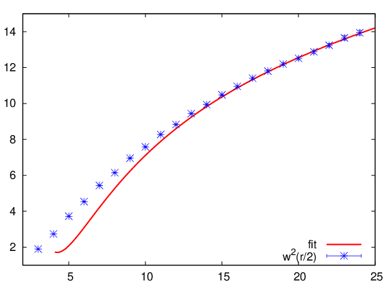
After determining the value of the string tension from the static potential, there is only one free parameter in eq.(4): from the fit, we obtain .
In the numerical results discussed so far, the plaquette orientation is parallel to the plane of the quark worldlines. However, one can also consider other orientations for the plaquette in eq.(15). Figure 3 shows the normalized probability distribution for the confining string using the three different orientations for the plaquette. The distance between the static sources is .

2.2 The linear broadening at finite temperature
In this subsection we investigate the dependence of the width of the flux tube on the distance between the static quarks at finite temperature. We again consider (2+1)-d Yang-Mills theory at . The lattice size is now which corresponds to a temperature of about , where is the temperature of the deconfinement phase transition.
It is important to note that the two low-energy constants, and , appearing in eq.(4) for the next-to-leading expression of the confining string width, have been already fixed by a fit to the data obtained at zero temperature. Hence, there is no longer an adjustable parameter to fit to the finite temperature numerical data and the theoretical prediction is completely determined. This represents a very stringent test of the validity of the low-energy effective string description of the confining string.

Figure 4 shows the dependence of the flux tube width on the separation between the two static quarks as it results from the numerical simulations. The two solid curves are the fully determined prediction eq.(4) of the low-energy effective string theory using the two choices . The numerical data show the predicted linear broadening for sufficiently large separations. The agreement with the analytic expression is excellent: this confirms in a quantitative manner the correctness of the description of the low-energy dynamics of the flux tube as a fluctuating string.
3 The confining string connecting color charges in larger representations
In Yang-Mills theory the gluons are the only dynamical degrees of freedom. One can probe their dynamics by inserting into the system external static color charges that transform under a given representation of the gauge group. Since gluons transform under the adjoint representation of the gauge group, -ality is a relevant concept to understand the behavior of color charges transforming under a generic representation of the gauge group. Let us consider the gauge group . Two representations and are in the same -ality sector if the second representation appears in the tensor product decomposition of with a given number of adjoint representations. This means that two color charges that transform under the representations and can transmute into one another by gluon exchange. For there are sectors: these -ality sectors are not independent but are pairwise related by charge conjugation symmetry (real and pseudoreal representations are self-related).
Let us now insert into the system a quark-anti-quark pair transforming under a given representation of the gauge group. The color flux tube that connects the two color sources is, in general, unstable and it decays when the two charges are pulled apart to a sufficiently large distance [29, 30, 31, 32, 33]. In every -ality sector there is just a single stable flux tube: it is the one with the minimal value of the string tension. These stable strings are known as -strings, where labels the -ality sector.
The internal structure of the flux tube connecting color sources transforming under larger representations of the gauge group is not known. Hence, it is not clear how to extend the low-energy effective theory of the confining string connecting two fundamental charges to those cases.
For , -strings are expected to consist of non-interacting fundamental strings. In that limit, the low-energy regime of -strings is described by replicas of the effective string connecting two fundamental color charges. For large, but finite , it is reasonable to expect that the fundamental strings are weakly interacting. If is the energy scale of such an interaction, then one would expect to observe two different low-energy regimes. In the energy range — where is the fundamental string tension — the effective picture of non-interacting fundamental strings may be a meaningful description. However, for energies smaller than , the bunch of fundamental strings merge and effectively behave like a single flux tube. Then it is appropriate to consider the effective theory of a single string with the string tension of the -string as a low-energy parameter. Moreover, when is not large, it may not be justified to view the -string as a composite object of fundamental strings and it is not clear what the appropriate low-energy description of the confining flux tube is.
In the next two subsections, we report on numerical results of Monte Carlo simulations of Yang-Mills theory with color sources in larger representations of the gauge group. In the first subsection results for -strings are discussed. In the second subsection the decay of unstable strings is investigated.
3.1 The effective string theory for -strings
In this subsection we present the results of numerical investigations on string effects for -strings. In and Yang-Mills theories, the confining string connecting two fundamental color charges is the only stable string. Here we consider Yang-Mills theory because it is the simplest pure gauge theory with a second stable confining string. In fact the 2-string connecting two color charges in the representation of cannot break and it does not belong to the -ality sector of the fundamental representation. Since it is least problematical for numerical simulations, we perform this study in (2+1) dimensions: we consider a lattice at In order to extract informations on the low-energy regime of the 2-string, we measure the Lüscher term. We expect to observe one of the following cases. If the 2-string consists of two non-interacting fundamental strings, then the coefficient of the Lüscher term should be twice the coefficient of the string connecting two fundamental charges. If the two fundamental strings are strongly interacting or, eventually, if the 2-string cannot even be interpreted as a bound state of fundamental strings, then the Lüscher term should be the same as the one of the fundamental string. However, also other results may be obtained [34]. Numerical results of Teper and collaborators [10, 11] support that the Lüscher term of the 2-string is the same as the one of the fundamental string. Here we perform an accurate comparison of the Lüscher term for the fundamental string and the 2-string. In particular we focus on the dependence on the separation between the two static sources.

Figure 5 shows the force as a function of the distance, both for the fundamental string and the 2-string. The solid curve is a fit of the form of the data for the fundamental string. We obtain the value for the fundamental string tension. Then the dashed and the dotted lines correspond to the predictions of the string tension of the 2-string assuming the Casimir law [35, 36] and the sine law [37], respectively. The data for the force of the 2-string happen to be in-between those two laws.

Figure 6 reports the value of for the fundamental string and the 2-string
| (19) |
For large separations between the color sources, the quantity approaches asymptotically the coefficient of the Lüscher term. The data for the 2-string accurately confirm that, for sufficiently large distances, the 2-string behaves like a single bosonic string: the quantity indeed approaches the value just like the fundamental string. However, it turns out that for not very large distances, there are important deviations from the asymptotic value. This might suggest that, as becomes large, the approach to happens at larger and larger distances and a different regime may eventually appear at intermediate separations between the static sources.
3.2 String decay
In this subsection, we investigate the behavior of unstable strings as the distance between the static color sources is increased. For simplicity, we consider the Yang-Mills theory in (2+1) dimensions. The only stable string is the one connecting two color charges in the fundamental representation: all other confining strings either decay into the fundamental one or break. Adjoint color sources — i.e. charges in the representation of — belong to the -ality sector of the trivial representation. As we pull apart a pair of adjoint sources, the confining string that connects the two static sources is being stretched. However, at sufficiently large distances, the string breaks and the static potential flattens [29, 30, 31, 32].
Color sources in the representation cannot be completely screened by gluons. Hence the confining string connecting two charges does not break completely but decays into the fundamental string. The string connecting two charges in the representation ultimately breaks. However, at intermediate distances, dynamical gluons can partially screen the charges so that they behave as effective color charges in the adjoint representation. Thus, the initial string can undergo multiple decays with a progressive partial screening at every decay step [33].
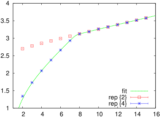
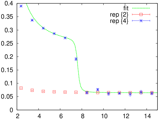
We show here the data of numerical simulations of (2+1)-d Yang-Mills theory on a lattice at coupling . The left-panel of figure 7 compares the static potentials of two charges and two fundamental charges. At distances , the charges get screened: they behave as two fundamental charges and the string decays. In fact, after the string decay, the static potential is the same as that of two fundamental charges. In the right-panel of figure 7 we display the results for the force. The data give evidence that, after the decay of the string, the string tension takes the value of the fundamental string tension.
The left-panel of figure 8 reports the results for the static potential of and color charges. The data for the representation show that indeed charge screening takes place in partial steps. The charge is first partially screened to behave as an effective charge: this is what the first kink in the static potential shows. As we can see in the right-panel of figure 8, after the first decay of the string, the value of the force agrees with the force between two charges. At the second decay the string breaks completely and the string tension vanishes.
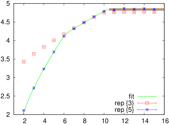

Interestingly, there is a small difference between the flattening levels of the and of the static potentials. This is most probably due to the different gluon content of the doubly screened charge and of the singly screened charge.
It is interesting to extend the investigation of the string decay also to other groups than . For instance groups [38] have only two -ality sectors like . The fundamental representation of is and is the adjoint representation. Interestingly, has a center-neutral representation with smaller dimensionality than the adjoint: it is , the fundamental representation of . Since the decomposition of the tensor product of and the adjoint representation is given by
| (20) |
the charge needs two gluons to be completely screened. Moreover it is reasonable to expect that the string tension between two charges is smaller than the one between two adjoint charges: thus, the string breaks in a single step with the simultaneous dynamical production of 4 gluons.
Another interesting example is related to the fundamental charge of . In Yang-Mills theory [39] there are no stable strings and all confining strings ultimately break. A fundamental charge is completely screened by 3 gluons, belonging to the representation . However, the fundamental representation is the smallest representation of the group and the confining string connecting two charges has the minimal string tension [15]. Thus, partial screening of the fundamental charge cannot happen: the string breaks in just one step by popping out from the vacuum 6 gluons [16].
4 Conclusions
In this paper we have presented recent results in the investigation of string effects in Yang-Mills theory. We have discussed confining strings connecting fundamental charges as well as color sources transforming under larger representations of the gauge group.
The color flux tube connecting two fundamental charges broadens as the separation of the static sources is increased. We have performed numerical simulations in (2+1)-d Yang-Mills theory both at zero and at finite temperature. At zero temperature we have shown that the width of the confining string increases logarithmically, in very good agreement with the analytic results obtained in the low-energy effective string theory for the color flux tube. The 2-loop expression for the width obtained using the low-energy effective string theory involves two low-energy constants: the string tension and a distance scale . The string tension has been fixed using the static potential and, thus, the fit of the numerical data for the width has only one free parameter.
The low-energy effective string theory also predicts that the flux tube broadens linearly at finite temperature. The numerical simulations have confirmed this expectation to very high accuracy. It is remarkable that, after having fixed the value of and using the zero temperature results, the prediction obtained in the low-energy effective string theory is completely determined.
Then the confining strings connecting color charges transforming under larger representations of the gauge group have been investigated. For stable strings — the so-called -strings — we have investigated the Lüscher term. We have performed numerical simulations of (2+1)-d Yang-Mills theory and measured with high accuracy the static potential for and color charges. The coefficient of the Lüscher term for the string approaches the value of the fundamental string for large separations of the color charges. However, at shorter distances, relevant deviations from the asymptotic value are observed. This result could suggest that, for large , some intermediate regime may appear.
Concerning unstable strings, we have investigated the decay of confining strings in (2+1)-d Yang-Mills theory. We have presented evidence for the decay of a string state into another string state and for multiple decays resulting from the progressive partial screening of color charges transforming under larger representations.
Acknowledgments.
The results presented in this paper have been obtained in collaboration with F. Gliozzi and U.-J. Wiese. I would like to thank them for many insightful discussions over the years and for critical reading of this paper. I also thank A. Amato for a useful remark.References
- [1] M. Lüscher, K. Symanzik, and P. Weisz, Nucl. Phys. B173 (1980) 365.
- [2] M. Lüscher, Nucl. Phys. B180 (1981) 317.
- [3] M. Hasenbusch and K. Pinn, Physica A192 (1993) 342.
- [4] M. Caselle, R. Fiore, F. Gliozzi, M. Hasenbusch, and P. Provero, Nucl. Phys. B486 (1997) 245.
- [5] K. J. Juge, J. Kuti, and C. Morningstar, Phys. Rev. Lett. 90 (2003) 161601.
- [6] M. Lüscher and P. Weisz, JHEP 0207 (2002) 049.
- [7] M. Caselle, M. Pepe, and A. Rago, JHEP 0410 (2004) 005.
- [8] M. Caselle, M. Hasenbusch, and M. Panero, JHEP 0603 (2006) 084.
- [9] N. D. Hari Dass and P. Majumdar, JHEP 0610 (2006) 020.
- [10] B. Bringoltz and M. Teper, Phys. Lett. B663 (2008) 429.
- [11] A. Athenodorou, B. Bringoltz, and M. Teper, JHEP 0905 (2009) 019.
- [12] B. B. Brandt and P. Majumdar, Phys. Lett. B682 (2009) 253.
- [13] M. Lüscher, G. Münster, and P. Weisz, Nucl. Phys. B180 (1981) 1.
- [14] M. Shifman, Acta Phys. Polon. B36 (2005) 3805.
- [15] L. Liptak and S. Olejnik, Phys. Rev. D78 (2008) 074501.
- [16] B. H. Wellegehausen, A. Wipf, and C. Wozar, arXiv:1006.2305 [hep-lat].
- [17] M. Lüscher and P. Weisz, JHEP 0407 (2004) 014.
- [18] O. Aharony and E. Karzbrun, JHEP 0906 (2009) 012.
- [19] O. Aharony and M. Field, arXiv:1008.2636 [hep-th].
- [20] O. Aharony and N. Klinghoffer, arXiv:1008.2648 [hep-th].
- [21] F. Gliozzi, M. Pepe, and U.-J. Wiese, arXiv:1006.2252 [hep-lat].
- [22] A. Allais and M. Caselle, JHEP 0901 (2009) 073.
- [23] M. Caselle, JHEP 1008 (2010) 063.
- [24] A. S. Bakry, D. B. Leinweber, P. J. Moran, A. Sternbeck, and A. G. Williams, arXiv:1004.0782 [hep-lat].
- [25] R. Sommer, Nucl. Phys. B411 (1994) 839.
- [26] M. Lüscher and P. Weisz, JHEP 0109 (2001) 010.
- [27] F. Gliozzi, M. Pepe, and U.-J. Wiese, Phys. Rev. Lett. 104 (2010) 232001.
- [28] F. Gliozzi, M. Pepe, and U.-J. Wiese, arXiv:1010.1373 [hep-lat].
- [29] G. I. Poulis and H. D. Trottier, Phys. Lett. B400 (1997) 358.
- [30] P. W. Stephenson, Nucl. Phys. B550 (1999) 427.
- [31] O. Philipsen and H. Wittig, Phys. Lett. B451 (1999) 146.
- [32] S. Kratochvila and P. de Forcrand, Nucl. Phys. B671 (2003) 103.
- [33] M. Pepe and U.-J. Wiese, Phys. Rev. Lett. 102 (2009) 191601.
- [34] P. Giudice, F. Gliozzi, and S. Lottini, JHEP 0705 (2007) 010.
- [35] J. Ambjorn, P. Olesen, and C. Peterson, Nucl. Phys. B240 (1984) 189.
- [36] J. Ambjorn, P. Olesen, and C. Peterson, Nucl. Phys. B240 (1984) 533.
- [37] A. Hanany, M. J. Strassler, and A. Zaffaroni, Nucl. Phys. B513 (1998) 87.
- [38] K. Holland, M. Pepe, and U.-J. Wiese, Nucl. Phys. B694 (2004) 35.
- [39] K. Holland, P. Minkowski, M. Pepe, and U.-J. Wiese, Nucl. Phys. B668 (2003) 207.