Hot Jupiter Magnetospheres

Hot Jupiters, the gas giant exoplanets found at small orbital radii, $D\lesssim 0.1\ {\rm AU}$, present an opportunity to study planets orbiting in an extreme environment very close to their parent stars. They experience insolation levels $\sim 10^{4}$ times greater than solar system gas giants. As a consequence of the high temperatures generated by EUV heating, the gas pressure scale height is comparable to the planetary radius, creating an extended upper atmosphere of gas potentially observable through transmission or reflection spectroscopy. Heating may also create an outward pressure force, complemented by outward centrifugal and tidal forces, which may drive an outflow leading to mass and angular momentum loss from the planet.

While most observational effort for the transiting planets has centered on the lower atmosphere, near the photospheres for optical and infrared continuum radiation at mbar-bar pressures, there has also been progress in probing higher levels in the atmosphere. As these observations probe a larger area surrounding the planet, the transit depth is correspondingly larger than that from the photospheric radius, $R_{\rm ph}$. Bound-bound atomic lines in the transmission spectrum from NaI [8], HI [48, 47, 11], OI and CII [47], and SiIII [27] have been observed for HD 209458b; HI in HD 189733b [25]; and MgII [14], and possibly other species at lower signal to noise, in WASP-12b. Bound-free transitions from a population of hydrogen in the $n=2$ state have been detected in the transmission spectrum of HD 209458b [3], although no bound-bound transitions from $n=2$ were found [50].

The large transit depths observed for the Lyman $\alpha$ line in HD 209458b imply neutral H atoms occupy an occulting area equivalent to an optically thick disk extending out to several planetary radii, comparable to the Roche-lobe radius for this close-in planet. This led Vidal-Madjar et al. [48] to suggest that the H atoms are escaping from the planet, as they would no longer be bound to the planet outside the Roche-lobe radius. The presence of heavy atoms (C, O, etc.), whose scale height should be far smaller than that of the H atoms, was suggested to be due to a combination of efficient turbulent mixing and drag forces from the escaping gas, entraining the heavier elements in an outflow [47, 15]. Ben-Jaffel [4] used archival HST data to rederive the transit depth, and challenged the claim that atmospheric escape was occurring, due to a derived transit depth that would imply the H atoms are within the Roche lobe radius. Two subsequent studies [5, 49] elucidated the dependence of transit depth on the analysis method and wavelength range studied. The recent study by Linsky et al. [27] attempts to constrain the wind velocity in HD 209458b using the line profiles for the CII and SiIII lines.

Most theoretical efforts to explain the aforementioned observations invoke EUV heating to temperatures $\sim 10^{4}\ {\rm K}$, creating a thermally driven, possibly transonic hydrodynamic outflow from the planet [54, 55, 46, 15, 34, 45]. While initiated by outward gas pressure gradients, a thermally-driven wind can be significantly accelerated by the tidal gravity¹¹ 1 In this paper we will use the phrase“tidal gravity” to include the effect of both the stellar tide and the centrifugal force, assuming synchronized rotation (see § V.). An alternative model is to treat atmospheric escape as Roche-lobe overflow [17, 26, 23], assuming that the fluid can only reach the sound speed in the vicinity of the L1 Lagrange point.

For gas giants, H is the most abundant element and heating is dominated by photoionization of atomic H in the thermosphere [54]. Photoionization leads to significantly ionized gas at high altitudes that is subject to magnetic forces. In light of the high ionization fraction, the planetary magnetic field, due to dynamo action in the planet’s core, may be dynamically important and affect density and velocity profiles in the upper atmosphere. This paper is a first attempt to include the effects of the planet’s magnetic field combined with tidal and centrifugal forces on upper atmosphere structure for hot Jupiters.

We model the magnetized, hot, rotating portion of the planet’s upper atmosphere in the context of magnetohydrodynamic (MHD) outflows, the theory of which was originally developed for stars and accretion disks. Figure 1 shows a cartoon of the expected structure for the wind from an isolated object with a surface dipole field: the polar region supports an outflow while the equatorial region contains static, magnetically confined gas [54, see also]. This configuration applies interior to the magnetosphere-stellar wind interaction, for planets not too near the parent star. Near the parent star, tidal forces are an important consideration, and we will show that tides may strongly affect the density profile and size of the static region, and may even shut the wind off in the polar region.

In the first half of the paper (§ II through § VII), we develop a general theory of isothermal hot Jupiter magnetospheres. Section II discusses the problem setup and approximations used to obtain a solution. Planetary magnetic field strengths predicted by dynamo models are discussed in section III. Section IV discusses qualitative features of atmospheric structure, and motivation for the existence of a dead zone. Section V reviews the centrifugal and tidal forces, and discusses the projection of these forces along magnetic field lines. The structure of the dead zone is discussed in section VI, followed by the wind zone in section VII.

The second half of the paper (§ VIII through § XII) uses the Lyman $\alpha$ transmission spectra to constrain parameters of the global 3D models. In section VIII, we construct a 1D model in hydrostatic, thermal, and ionization balance to compute appropriate values for the base pressure and temperature for the 3D global models that we present in section IX. Mass loss rates are computed and spin-down torques are estimated, in section X. Neutral H column density maps for the global models are used to illustrate the dependence on key parameters in section XI. Lyman $\alpha$ transmission spectra in comparison with observations and scattering of stellar Lyman $\alpha$ by the planet are presented in section XII. Finally, we compare and contrast our magnetic wind model with the standard Roche-lobe overflow model in section XIII. Summary and discussion are given in section XIV. The MHD wind equations and ion-neutral coupling are discussed in Appendices A and B, respectively.

In this section we outline the problem to be solved, and the simplifying assumptions used to find solutions. Except for section VIII, this paper discusses a 3D isothermal model of the upper atmosphere. The isothermal model is parametrized by an effective sound speed, as well as the pressure at a fiducial radius. Appropriate values for these parameters are discussed in a simple 1D spherical model in section VIII, including photoionization and thermal equilibrium.

In the 3D model, we compute approximate solutions of the one-fluid MHD equations with an inner boundary at the base of the warm H layer, and an outer boundary which extends to at least ten planetary radii (or one stellar radius). We treat the gas as having constant isothermal sound speed $a=\sqrt{k_{b}T/\mu m_{p}}$, where $T$ is gas temperature of the fluid, $\mu$ is the mean molecular weight, $k_{b}$ is Boltzmann’s constant, and $m_{p}$ is the proton mass. At the inner boundary, the density and pressure are assumed to follow equipotentials. We assume the planet’s rotation rate is synchronized with its orbital motion around the parent star, giving orbital and spin angular velocity $\Omega$. We work in a coordinate system centered on the planet and rotating at rate $\Omega$. The stellar gravity is included in the tidal approximation, and an effective potential $U$ is composed of the planetary gravity, stellar gravity, and the centrifugal force. We specify a specific magnetic field geometry which is dipole near the planet and matches onto a radial field at the dead zone radius. We compute the ionization fraction with a simple, optically thin model applied to the derived gas densities of the MHD model. To summarize, we have made several simplifying assumptions in order to focus on the new physics arising from MHD effects. We now discuss these simplifying approximations in more detail.

The simultaneous inclusion of photoionization heating, chemical reactions and collisional coupling between different species, stellar tidal forces, and the simultaneous interaction with the stellar wind in the presence of magnetic field is a formidable problem. Our approach is to first ignore the interaction with the stellar wind, but to include the effect of the stellar tidal forces felt by the planet’s atmosphere. The interaction with the stellar wind may alter the results of this paper in several ways [34, 45, see e.g.,]. The stellar wind will limit the size of the magnetosphere, as determined by stress balance at the magnetopause [41, e.g.,]. Reconnection between field lines in the stellar wind and magnetosphere may lead to magnetospheric convection, limiting the high density region to be inside a plasmapause [39], as for Earth. Finally, reconnection may also generate non-thermal plasma populations. We do not consider the interaction with the stellar wind in order to construct the simplest possible model.

Another key approximation is that we treat photoionization heating as being spherically symmetric, creating a hot layer uniformly over the planet. In reality, the night side temperature and ionization state may depend on day-night heat redistribution, and downward heat conduction along field lines not in the planet’s shadow. In perfect MHD, such redistribution would be highly constrained in the magnetically dominated upper atmosphere, but finite conductivity may allow field lines to slip through the gas [16]. Even on the day side, large gas density outside the Roche lobe may project a non-spherically symmetric shadow on the deeper layers.

Near the planet, the dynamo-generated, roughly dipole field from the planet’s core is expected to dominate. Moving outward, currents generated in the magnetosphere comb the field lines into a nearly radial direction beyond the dead zone radius. Such a geometry has been used before in the context of the stellar wind [31, 32, 38] and we will adopt it here. This field geometry will be implemented in the global models presented in section 9, and is motivated in the discussion of Appendix A.

Finally, the one-fluid approximation assumes that mean free paths are sufficiently small that relative motion of different species can be ignored. In Appendix B we will check this assumption a posteriori for our models, which estimate particle densities and velocities in the dead and wind zones. Specifically, we will show that the electron-proton-hydrogen atom gas is well coupled collisionally for the parameters of interest, and therefore the drift velocity is small and hydrogen atoms have short mean free paths in the dead zone region. As a consequence, neutral hydrogen atoms do not fly ballistically through the magnetosphere, and photoionization equilibrium is a good approximation when computing the ionization fraction. Further, we compute the rate at which magnetic field can drift relative to the fluid. For this thermal population of particles in the magnetosphere, we find that the dead zone gives the largest observable transit signal, and that the bulk of the hydrogen atoms in the dead zone are not escaping.

In the next section we will review expected magnetic field strengths for hot Jupiters.

The importance of the magnetic field for the upper atmosphere depends critically on the field strength. However, the magnetic fields of hot Jupiters are currently unconstrained by observation. This section will use theoretical considerations to estimate likely field strengths for hot Jupiters.

Sánchez-Lavega [42] computed that Rayleigh numbers in hot Jupiters are typically much larger than the critical Rayleigh number for thermal convection in the metallic core. Using estimates of the fluid velocity carrying the heat flux, he found that the magnetic Reynolds number is much larger than unity, and that dynamo action can occur. He argued that if the dynamo operated with Elsasser number of order unity, then $B\sim(2\rho\Omega\lambda_{B})^{1/2}$, where $\rho$ is the mass density and $\lambda_{B}$ is the magnetic diffusivity. The dominant scaling important for hot Jupiters is then with rotation: $B\propto\Omega^{1/2}$. For synchronized planets with orbital periods of a few days, this scaling predicts that the field for hot Jupiters should be smaller than that of Jupiter (equatorial field $B_{\rm J,eq}=4.3\ {\rm G}$) by a factor of a few.

The opposite conclusion may be drawn from the recent results of Christensen et al. [9]. As the rotation rate is increased above a critical value, the field strength no longer increases with rotation rate, and dynamo simulations give a magnetic field strength $B\sim(\rho F_{\rm core}^{2})^{1/3}$, nearly independent of rotation rate and magnetic diffusivity, where $F_{\rm core}$ is the heat flux escaping from the conducting core. Christensen et al. [9] show that this scaling applies to both planets and rapidly rotating, low mass stars over many orders of magnitude in heat flux. They argue that the dependence on $F_{\rm core}$ arises since it is the heat flux reservoir that sustains the magnetic field against Ohmic dissipation. To be in the saturated regime, the Rossby number $Ro$ must satisfy $Ro=V_{\rm ed}/\Omega\ell\lesssim 0.1$, where $V_{\rm ed}$ is the typical velocity of the eddies transporting heat, and $\ell$ is the size of the conducting region; $\ell\sim R$ for $M_{p}\gtrsim 0.5M_{J}$. Sánchez-Lavega [42] estimated synchronized planets in few day orbits to have $Ro\ll 0.1$, using heat fluxes comparable to that of Jupiter. Hence these planets are expected to be in the saturated regime.

The large radii of hot Jupiters are currently not well understood, since the cooling and contraction time for passively cooling planets, even allowing for irradiation by the star, is far shorter than the age for a number of observed planets [13, e.g.,]. This has led to the suggestion that these planets are not passively cooling, but rather have an anomalous source of internal heating, which is as yet unidentified but balances the core cooling rate. To assess the required heating rates, Arras & Socrates [2] computed cooling flux from the core for planets as a function of radius [their Figure 11; see 1, for a discussion of the cooling luminosity of irradiated hot Jupiters]. For Jupiter-mass planets in the radius range $R_{\rm ph}=1.3-1.5R_{J}$, the cooling flux is larger than that of Jupiter by a factor $10^{2}-10^{3}$, for which the Christensen et al. [9] scaling would give magnetic fields $5-10$ times larger than Jupiter. Larger mass planets with the same radius would have larger cooling fluxes, and vice versa. For instance, WASP 12b, WASP 17b and TRES 4 have radii $R_{\rm ph}\sim 1.8R_{J}$ and masses in the range $0.5-1.5M_{J}$²² 2 http://exoplanet.eu/catalog-transit.php, for which the cooling fluxes would be $10^{3}-10^{4}$ times higher than Jupiter, implying fields larger than Jupiter by factors of $10-20$.

In summary, the recent results on dynamo theory from Christensen et al. [9], and the assumption that hot Jupiter cores are subject to an externally powered heating [2], argue that field strengths may be up to an order of magnitude larger than that of Jupiter. We will take this as motivation to explore a wide range of parameter space for the magnetic field in our calculations.

In the next section, we show that the photoionized H and H⁺ layers are magnetically dominated for field strengths comparable to Jupiter or Saturn, and motivate the existence of a dead zone by a toy problem.

Yelle [54] and [15] presented detailed calculations of the transition between the molecular lower atmosphere (H₂), the layer dominated by atomic hydrogen (H), and the ionized upper atmosphere (H⁺). In this paper, we restrict attention to the H and H⁺ regions, where the transmission spectrum is formed. The strong heating in these layers due to UV photon energy deposition raises the temperature to $T\simeq 10^{4}\ {\rm K}$. As a consequence of the increased temperature and low mean molecular weight, the radial extent of the H and H⁺ layers ($\gtrsim R_{J}$) is expected to be much larger than that of the H₂ layer above the photosphere ($\lesssim(0.1-0.2)\times R_{J}$).

We define the lower boundary of our wind model to be at the base of the warm ($T\gtrsim 5000\ {\rm K}$) H layer, at base radius $R$ and base pressure $P_{\rm base}$. The base of the warm layer is a crucial parameter for the transit depth. As discussed in the phenomenological model of Koskinen et al. [22], the transit depth of HD 209458b could be understood as being due to thermal $\simeq 10^{4}\ {\rm K}$ H gas extending down to $\sim 10-100\ \rm nbar$ pressures. In section VIII, we compute a simple 1D model for ionization and thermal equilibria in the H and H⁺ layers which shows that such base conditions are indeed possible.

The Lyman $\alpha$ transmission spectrum of HD 209458b shows absorption by the planetary atmosphere at linewidths $\Delta v\gtrsim 100\ \rm km\ s^{-1}$ from line center. At this linewidth, the cross section is $\sigma_{\nu}\simeq 2\times 10^{-19}\ \rm cm^{2}$ (see Figure 15). Optical depth unity requires a hydrogen column $N_{H}\simeq 1/\sigma_{\nu}\simeq 5\times 10^{18}\ \rm cm^{-2}$. Assuming the gas is dominated by atomic hydrogen, the pressure at this level in the atmosphere is $P\simeq gm_{p}N_{H}\simeq 2\ {\rm nbar}\ (g/300\ \rm cm\ s^{-2})$ (see Figure 10). This is a factor $\sim 10^{8}$ more rarefied than the optical photosphere for continuum radiation at pressure $P_{\rm ph}\simeq{\rm 100\ mbar}$. Magnetic forces dominate in this layer if $B^{2}/8\pi\gtrsim 2\ {\rm nbar}\ (g/300\ \rm cm\ s^{-2})$, implying a critical field strength $B_{\rm crit}\gtrsim 0.25\ {\rm G}\ (g/300\ {\rm cm^{2}\ s^{-1}})^{1/2}$. This is less than Jupiter’s equatorial magnetic field $B_{\rm J,eq}=4.3\ {\rm G}$ and comparable to Saturn’s equatorial field $B_{\rm S,eq}=0.22\ {\rm G}$. Moving upward, if the gas pressure drops much faster than magnetic pressure, the atmosphere can become highly magnetically dominated — a magnetosphere.

The theory of thermally and magneto-centrifugally driven MHD winds gives guidance on the upper atmosphere structure in the magnetically dominated case (for a good review see Spruit 44). Consider a thought experiment in which a non-magnetic spherically symmetric wind with velocity $v_{\infty}$ and mass loss rate $\dot{M}$ exists at time $t<0$, and at time $t=0$ a dipole magnetic field is turned on. On which field lines can the wind overpower the magnetic forces and open the field lines to infinity? The magnetic pressure on the equator ($\theta=\pi/2$) is weaker than at the footpoint (at angle $\theta_{b}$) by a factor $[B(\pi/2)/B(\theta_{b})]^{2}=[R/r(\pi/2)]^{6}=\sin^{12}\theta_{b}$ (see eq.12). This powerful dependence on footpoint position means there are always field lines near the magnetic poles which open to infinity on which a wind can outflow (see Figure 1 for a cartoon). The reason is that at the equator, the wind ram pressure can overcome the steeply falling magnetic pressure at sufficiently large distance from the planet. If we assume the wind ram pressure decreases outward as $\rho v^{2}=\dot{M}v_{\infty}/4\pi r^{2}$, then the critical footpoint angle inside of which a “polar wind” occurs is $\sin\theta_{b}\simeq\left(\dot{M}v_{\infty}/R^{2}B_{0}^{2}\right)^{1/8}$. For fiducial polar magnetic field $B_{0}=8.6\ {\rm G}$, $R=1.4R_{J}$, (constant) flow speed $v_{\infty}=10\ {\rm km\ s^{-1}}$ and mass loss rate $\dot{M}=10^{11}\ {\rm g\ s^{-1}}$ (motivated by the studies of Yelle 54, García Muñoz 15, Murray-Clay et al. 34), we find the polar cap size occupied by open field lines is $\theta_{b}\simeq 14^{\circ}$, and the last closed field lines is at equatorial radius $r(\pi/2)\simeq 16R$. This static, closed field line region is referred to as the “dead zone” [31]. These estimates suggest that the region within a few planetary radii, where the transit signal arises, is filled primarily with static gas in the dead zone, rather than outflowing gas, as has been previously assumed.

For close-in, tidally-locked planets, tides and centrifugal forces play a key role in upper atmosphere structure. In the next section we review the effective potential near the planet, and the projection of forces along dipole field lines.

Gas in the upper atmosphere of the planet is subject to three potential forces: gravity from the planet, tidal gravity from the star, and the centrifugal force due to the planetary rotation. For a synchronized planet, the centrifugal and tidal forces, or just tidal force for short, are comparable in strength, although their angular dependence is different. For position vector $\mbox{\boldmath$\displaystyle x$}=(r,\theta,\phi)$ relative to the center of the planet, and star at position $\mbox{\boldmath$\displaystyle x$}_{\star}=(D,\pi/2,0)=D\mbox{\boldmath$\displaystyle e$}_{x}$, the sum of the three accelerations is

$\displaystyle\mbox{\boldmath$\displaystyle a$}(\mbox{\boldmath$\displaystyle x$})$

$\displaystyle=$

$\displaystyle-{\mbox{\boldmath$\nabla$}}U(\mbox{\boldmath$\displaystyle x$}),$

(1)

where the effective potential is given by

	$\displaystyle U(\mbox{\boldmath$\displaystyle x$})$	$\displaystyle=$	$\displaystyle-\frac{GM_{p}}{|\mbox{\boldmath$\displaystyle x$}|}-\frac{GM_{\star}}{|\mbox{\boldmath$\displaystyle x$}-\mbox{\boldmath$\displaystyle x$}_{\star}|}+\frac{GM_{\star}\mbox{\boldmath$\displaystyle x$}\cdot\mbox{\boldmath$\displaystyle x$}_{\star}}{|\mbox{\boldmath$\displaystyle x$}_{\star}|^{3}}-\frac{1}{2}\left|\mbox{\boldmath$\displaystyle\Omega$}\times\mbox{\boldmath$\displaystyle x$}\right|^{2}$		(2)
		$\displaystyle\simeq$	$\displaystyle-\frac{GM_{p}}{r}-\frac{1}{2}\Omega^{2}r^{2}\left(f\sin^{2}\theta-1\right).$		(3)

Equipotentials are shown in Figure 6.2 of Kopal [21]. The longitude-dependent function $f=1+3\cos^{2}\phi$. The vector angular velocity of the orbit is $\mbox{\boldmath$\displaystyle\Omega$}=\Omega\mbox{\boldmath$\displaystyle e$}_{z}$, where $\mbox{\boldmath$\displaystyle e$}_{z}$ is normal to the orbital plane, and $\Omega=[G(M_{\star}+M_{p})/D^{3}]^{1/2}$. The first and second terms in eq.2 are the potential of the planet and star, respectively. The third term in eq.2 is due to the motion of the origin of the coordinate system. The last term in eq.2 is due to the centrifugal force. It may be shown that eq.2 is equivalent to the usual Roche potential with origin at the center of mass by combining the third and fourth terms. The form in eq.3 is an expansion in the limit $r\ll D$, and agrees with that for “Hill’s limit” found in Murray & Dermott [35] when evaluated in the orbital plane ($\theta=\pi/2$).

The accelerations are given by

	$\displaystyle a_{r}$	$\displaystyle=$	$\displaystyle-\frac{\partial U}{\partial r}=-\frac{GM_{p}}{r^{2}}+\Omega^{2}r\left(f\sin^{2}\theta-1\right),$		(4)
	$\displaystyle a_{\theta}$	$\displaystyle=$	$\displaystyle-\frac{1}{r}\frac{\partial U}{\partial\theta}=f\Omega^{2}r\sin\theta\cos\theta$		(5)
	$\displaystyle a_{\phi}$	$\displaystyle=$	$\displaystyle-\frac{1}{r\sin\theta}\frac{\partial U}{\partial\phi}=-3\Omega^{2}r\sin\theta\sin\phi\cos\phi.$		(6)

The vector acceleration $\displaystyle a$ should not be confused with the sound speed $a$. If we denote the coordinate along the star-planet line $x=r\sin\theta\cos\phi$, and normal to the orbit plane $z=r\cos\theta$, then the tidal force is outward when $3x^{2}>z^{2}$, i.e. within latitudes $-\pi/3$ to $\pi/3$ of the equator. The tidal force is zero in the $y$-direction. Hence when observing a planet in the plane of the sky during transit, the tidal forces are inward along $\mbox{\boldmath$\displaystyle e$}_{z}$, zero along $\mbox{\boldmath$\displaystyle e$}_{y}$, and away from the planet along $\mbox{\boldmath$\displaystyle e$}_{x}$, the line of sight during transit.

The L1 and L2 Lagrangian points at radii $r_{\rm L1}$ and $r_{\rm L2}$ are found by using eq.4 along the star-planet line ($\theta=\pi/2,\phi=0$), giving

$\displaystyle r_{\rm L1}\simeq r_{\rm L2}\simeq r_{\rm L}$

$\displaystyle\equiv$

$\displaystyle D\left(M_{p}/3M_{\star}\right)^{1/3}=(GM_{p}/3\Omega^{2})^{1/3}.$

(7)

The near equality $r_{\rm L1}\simeq r_{\rm L2}$ is due to $M_{\rm p}/M_{\star}\ll 1$ in eq.7. The photospheres of the observed planets are inside the L1-L2 radii.

How does the magnetic field alter the radius beyond which the net gravity points outward? What is needed is the projection $a_{\parallel}=\mbox{\boldmath$\displaystyle a$}\cdot\mbox{\boldmath$\displaystyle b$}$ along field lines, where $\mbox{\boldmath$\displaystyle b$}=\mbox{\boldmath$\displaystyle B$}/B$ is the unit vector along the magnetic field direction. In dipole geometry, approximately correct near the planet,

$\displaystyle B$

$\displaystyle=$

$\displaystyle B_{0}\left(\frac{R}{r}\right)^{3}\left(\mbox{\boldmath$\displaystyle e$}_{r}\cos\theta+\mbox{\boldmath$\displaystyle e$}_{\theta}\frac{\sin\theta}{2}\right).$

(8)

and the unit vector is

$\displaystyle b$

$\displaystyle=$

$\displaystyle\frac{1}{N}\left(\mbox{\boldmath$\displaystyle e$}_{r}\cos\theta+\mbox{\boldmath$\displaystyle e$}_{\theta}\frac{\sin\theta}{2}\right)$

(9)

where the normalization factor is

$\displaystyle N$

$\displaystyle=$

$\displaystyle\sqrt{\cos^{2}\theta+\sin^{2}\theta/4}=\sqrt{1-3\sin^{2}\theta/4}.$

(10)

The parallel acceleration is then

$\displaystyle a_{\parallel}$

$\displaystyle=$

$\displaystyle-\mbox{\boldmath$\displaystyle b$}\cdot{\mbox{\boldmath$\nabla$}}U=\frac{\cos\theta}{N}\left[-\left(\frac{GM_{p}}{r^{2}}+\Omega^{2}r\right)+\frac{3}{2}f\Omega^{2}r\sin^{2}\theta\right].$

(11)

The quantity in brackets in eq.11 must be positive in order for the net acceleration to be away from the planet. To solve for the radius at which the net acceleration is zero, we express $\theta$ in terms of $r$ along dipole field lines using

$\displaystyle r(\theta)$

$\displaystyle=$

$\displaystyle R\frac{\sin^{2}\theta}{\sin^{2}\theta_{b}}\equiv r_{\rm eq}\sin^{2}\theta$

(12)

where

$\displaystyle r_{\rm eq}$

$\displaystyle=$

$\displaystyle R/\sin^{2}\theta_{b}$

(13)

is the equatorial radius of the field line with footpoint at $\theta_{b}$. The “magnetic Roche lobe radius”, $r_{\rm RB}$, at which the projected acceleration $a_{\parallel}=0$ is given by the solution of the equation

$\displaystyle\frac{GM_{p}}{r_{\rm RB}^{2}}+\Omega^{2}r_{\rm RB}$

$\displaystyle=$

$\displaystyle\frac{3}{2}f\Omega^{2}\frac{r_{\rm RB}^{2}}{r_{\rm eq}}.$

(14)

Solutions can only exist in the range of radii $2r_{\rm eq}/3f\leq r_{\rm RB}\leq r_{\rm eq}$. Solutions for $r_{\rm RB}$ exist first at the looptop $r_{\rm RB}=r_{\rm eq}$ for loops of critical size

$\displaystyle r_{\rm eq,crit}$

$\displaystyle=$

$\displaystyle\frac{r_{\rm L}}{(f/2-1/3)^{1/3}}.$

(15)

That is, when the loop size becomes larger than about the L1-L2 distance, the outer part of the loop can have net acceleration pointing away from the planet. Note that this statement applies even in the plane where $\cos^{2}\phi=0$, where the radial component of the tidal force points inward. The magnetic geometry allows a “magnetic Roche lobe” $r_{\rm RB}\sim r_{\rm R}$ to exist at all longitudes, in contrast to the unmagnetized case.

In the next section we model the gas density in the dead zone.

The 3D MHD wind equations are presented in Appendix A. There we derive the Bernoulli constant along field lines and discuss how gas pressure discontinuities at the dead zone - wind zone boundaries give rise to current sheets which alter the magnetic field configuration. For the present section which discusses the dead zone, the main concept needed is that hydrostatic balance applies along field lines. We will approximate the field lines as dipolar.

In the dead zone, the velocity along field lines $\mbox{\boldmath$\displaystyle v$}=0$. Setting $\mbox{\boldmath$\displaystyle v$}=0$ in eq.A2 and dotting this equation with $\displaystyle b$ to eliminate the Lorentz force we find the equation of hydrostatic balance along field lines

$\displaystyle\frac{1}{\rho}\frac{dP}{ds}$

$\displaystyle=$

$\displaystyle a^{2}\frac{d\ln\rho}{ds}=-\frac{dU}{ds}$

(16)

where $d/ds=\mbox{\boldmath$\displaystyle b$}\cdot{\mbox{\boldmath$\nabla$}}$ is the derivative along field lines. Under the isothermal assumption, eq.16 can then be integrated to give the run of pressure and density along a field line with base position $(\theta_{b},\phi)$:

	$\displaystyle\frac{P(r,\theta,\phi)}{P(R,\theta_{b},\phi)}$	$\displaystyle=$	$\displaystyle\frac{\rho(r,\theta,\phi)}{\rho(R,\theta_{b},\phi)}$		(17)
		$\displaystyle=$	$\displaystyle\exp\left[-\left(\frac{U(r,\theta,\phi)-U(R,\theta_{b},\phi)}{a^{2}}\right)\right].$

We treat the density and pressure at the base as being along equipotentials. Defining $\rho_{ss}=P_{ss}/a^{2}=\rho(r=R,\theta=\pi/2,\phi=0)$ to be the value at the substellar point at the base radius, the density at the base radius at other points is

$\displaystyle\rho_{b}(\theta_{b},\phi)$

$\displaystyle=$

$\displaystyle\rho_{ss}\exp\left[-\left(\frac{U(R,\theta_{b},\phi)-U(R,\pi/2,0)}{a^{2}}\right)\right].$

(18)

Combining eq.17 and 18 then gives

	$\displaystyle\frac{P(r,\theta,\phi)}{P_{ss}}$	$\displaystyle=$	$\displaystyle\frac{\rho(r,\theta,\phi)}{\rho_{ss}}$		(19)
		$\displaystyle=$	$\displaystyle\exp\left[-\left(\frac{U(r,\theta,\phi)-U(R,\pi/2,0)}{a^{2}}\right)\right].$

Note that because we have assumed the density and pressure surfaces at the base are along equipotentials, eq.19 satisfies

$\displaystyle 0$

$\displaystyle=$

$\displaystyle-{\mbox{\boldmath$\nabla$}}P-\rho{\mbox{\boldmath$\nabla$}}U$

(20)

in all three directions, not just along field lines. In this case $-{\mbox{\boldmath$\nabla$}}U$ is balanced by gas pressure forces due to a non-spherical distribution of mass. If, on the other hand, temperature, density or pressure surfaces were not along equipotentials, then eq.20 would not be satisfied perpendicular to field lines, and the trans-field force balance (eq.A12) would be required to understand the required currents.

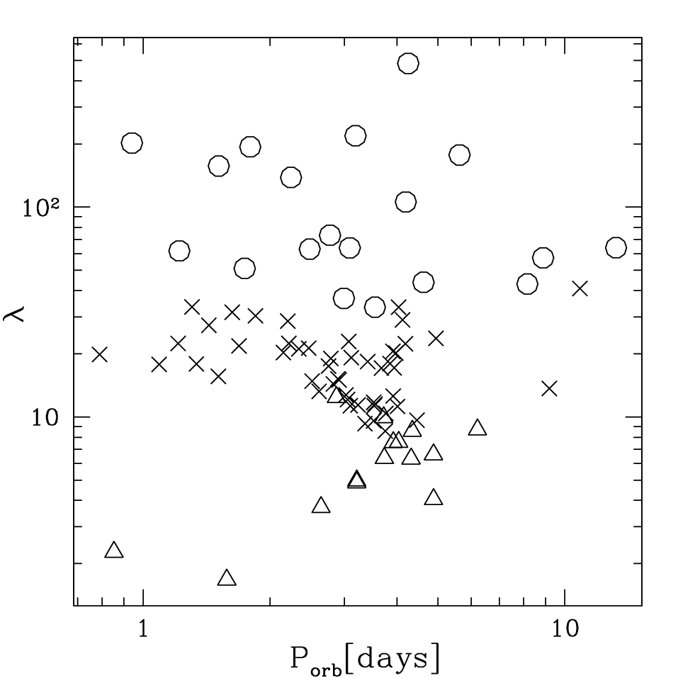
The potential difference in eq.19 can be written in dimensionless form

			$\displaystyle\frac{U(r,\theta,\phi)-U(R,\pi/2,0)}{a^{2}}$		(21)
		$\displaystyle=$	$\displaystyle\lambda\left(1-\frac{R}{r}\right)+\frac{1}{2}\epsilon\left[3-\left(\frac{r}{R}\right)^{2}\left(f\sin^{2}\theta-1\right)\right]$

where we have defined the ratio of escape to thermal speed

	$\displaystyle\lambda$	$\displaystyle=$	$\displaystyle\frac{GM_{p}}{Ra^{2}}$		(22)
		$\displaystyle\simeq$	$\displaystyle 9.3\left(\frac{M_{p}}{0.7M_{J}}\right)\left(\frac{1.4R_{J}}{R}\right)\left(\frac{10\ \rm km\ s^{-1}}{a}\right)^{2}$

and the ratio of rotation speed (or tidal potential) to thermal speed

	$\displaystyle\epsilon$	$\displaystyle=$	$\displaystyle\left(\frac{\Omega R}{a}\right)^{2}$		(23)
		$\displaystyle=$	$\displaystyle 0.043\left(\frac{\rm 3.5\ days}{P_{\rm orb}}\right)^{2}\left(\frac{R}{1.4R_{J}}\right)^{2}\left(\frac{10\ \rm km\ s^{-1}}{a}\right)^{2}.$

The photoionization model in section VIII shows outward increase in $T$ and decrease in $\mu$, implying larger $a$ with radius. The density will then decrease more slowly than in the isothermal model for the same quantities at the base.

Figures 2 and 3 show the values of $\lambda$ and $\epsilon$ versus planet orbital period for the transiting exoplanets, taking $M_{p}$, transit radius $R_{\rm ph}$ and orbital period $P_{\rm orb}=2\pi/\Omega$ from the Extrasolar Planets Encyclopedia³³ 3 http://exoplanet.eu/. The temperature and mean molecular weight have been set to fiducial values of $\mu=1$ and temperature $T=10^{4}\ {\rm K}$, giving sound speed of $a=9.3\ {\rm km\ s^{-1}}$.

Note that a substantial number of planets have $\lambda=2-10$, implying the scale height of the gas is large enough that the density decrease in the dead zone is only by a factor of $10-10^{4}$, far less than for planets with cold upper atmospheres more distant from their parent star. This increased density leads to the possibility that hot Jupiter upper atmospheres may be collisional to large distances from the planet, i.e. that the exobase, if it exists at all, is at radii $r\gg R_{\rm ph}$ [46, 34].

Next, note that for the same fiducial molecular weight and temperature, the strength of the tide, $\epsilon$, is in the range $0.1-1$ for a substantial number of planets. For large $\epsilon$, the typical rotational speed of a synchronized planet is comparable to the sound speed, or equivalently, the free fall speed in the tidal potential is comparable to the sound speed. Since $\epsilon$ is evaluated at the base, the tidal force will dominate even more at larger distances from the planet.

Figure 4 shows the run of gas and magnetic pressure along the equator ($\theta=\pi/2$) as a function of radius along the star-planet line ($\phi=0$). Eq.19 was used for the gas pressure, and eq.8 for the magnetic pressure. The magnetic pressure is parametrized by the plasma $\beta$ at the substellar point at the base:

$\displaystyle\beta$

$\displaystyle\equiv$

$\displaystyle\frac{8\pi P_{ss}}{(B_{0}/2)^{2}}=0.14\ \left(\frac{P_{ss}}{0.1\ \rm\mu bar}\right)\left(\frac{B_{\rm J,eq}}{B_{0}/2}\right)^{2}.$

(24)

The different lines in Figure 4 show gas pressure and magnetic pressure for different $\lambda$, $\epsilon$, and $\beta$ as a function of radius.

For small $\epsilon$, the density decreases outward, and eventually becomes a constant. When the tidal force is included the density increases outward for radii outside the magnetic Roche radius (eq.14), since the sign of gravity points outward there. This is a dramatic effect for close-in planets, whose Roche radii are at only a few planetary radii, and may lead to hydrogen densities orders of magnitude larger than the $\epsilon=0$ case. The tidal gravity plays a role similar to the centrifugal force in models of the closed field line regions in the solar wind [32] and in Jupiter’s magnetosphere outside the corotation radius. To specify the current and field distributions required for this support involves a solution of the trans-field equation, which is beyond the scope of this work. However, such support should be possible when magnetic pressure dominates gas pressure.

Next, we follow Mestel [31] and Mestel & Spruit [32] to estimate the size of the dead and wind zones. Pneuman & Kopp [40] showed that the dead zone ends at the equator in a cusp, i.e. the field in the dead zone approaches zero toward the cusp. Also, for $v\gtrsim a$, the wind zone pressure can be neglected compared to the dead zone pressure, leading to the condition (also see our discussion leading up to eq.A14 in Appendix A)

$\displaystyle P_{\rm dead}$

$\displaystyle\simeq$

$\displaystyle\frac{B_{\rm wind}^{2}}{8\pi}.$

(25)

To determine the cusp radius, which we call $r_{d}$ for dead zone, we use eq.19 for the left hand side and eq.8 for the right hand side. The resulting equation is

$\displaystyle\beta\exp\left[-\lambda\left(1-\frac{R}{r}\right)+\frac{3}{2}\epsilon\left(\frac{r^{2}}{R^{2}}\cos^{2}\phi-1\right)\right]=\left(\frac{R}{r}\right)^{-6}$

(26)

Eq.26 shows that the cusp radius will depend on $\phi$ in general due to the tidal potential. When tides can be ignored ($\epsilon\ll 1$), a reasonable approximation is $r_{d}/R\simeq(e^{\lambda}/\beta)^{1/6}$.

Figure 5 shows cusp radii as a function of $\beta$ for different tidal strength ($\epsilon$) and binding parameter ($\lambda$). Consider the fiducial case with $\epsilon=10^{-3}$, $\lambda=10$ and $\beta=10^{-2}$. Initially the magnetic pressure is much larger than the gas pressure. The more rapid decrease of magnetic pressure implies equality at the cusp radius, $r_{d}/R\simeq 10$. Increasing $\epsilon$, the gas pressure is larger and the cusp radius moves inward. The cusp radius moves outward with increasing magnetic field, i.e. decreasing $\beta$.

Under what conditions does a magnetosphere not form? Inspection of the $\beta=1$ and $\lambda=5$ curves in Figure 4 shows that the magnetic and gas pressures are initially equal at the base, but the gas density decreases more slowly and so the magnetic field never dominates. Ignoring tides, there is an analytic criterion for the critical $\beta_{\rm crit}=\beta_{\rm crit}(\lambda)$ for the formation of a dead zone. This criterion is found by requiring simultaneously $P=B^{2}/8\pi$ and $dP/dr=d/dr(B^{2}/8\pi)$, and yields $\beta\leq\beta_{\rm crit}=(6/\lambda)^{6}\exp(\lambda-6)$. For $\lambda=5,10,15$, the values are $\beta_{\rm crit}=1.1,2.5$ and $33$, agreeing with the cutoffs in Figure 5. Hence for large $\lambda$, the gas at the base need not be magnetically dominated in order for the gas well above to base to become so.

In summary, we have found cusp, or dead zone, radii in the range of a few to tens of radii $R$ for the expected range of $\lambda$, $\beta$ and $\epsilon$. Since transit observations to date probe the high density gas within a few planetary radii, these observations may be probing static gas trapped within the magnetosphere, as opposed to outflowing gas.

Nevertheless, as we will argue in section VII, a wind zone should exist, and we investigate its structure in the next section.

In this section we show how the (slow magneto-) sonic point is affected by the magnetic geometry. Readers unfamiliar with the MHD wind equations can consult Appendix A for a brief summary of the equations. We simplify the problem by assuming that the sonic point is close enough to the planet for magnetic stresses to dominate over hydrodynamic stresses — the rigid field line approximation. In this situation the fluid nearly corotates with the planet, and can be accelerated like “beads on a wire” by the magnetic field. This “magneto-centrifugal” effect from stellar wind theory [31] becomes important when the rotation velocity approaches the sound speed at the sonic point [32]. For a synchronized hot Jupiter, tidal forces are of comparable size as centrifugal forces, and the condition that the rotation velocity is comparable to the sound velocity at the sonic point is equivalent to the Roche-lobe radius being near the sonic point. The rigid field line assumption will typically break down near the Alfvén point, which we estimate lies well outside the dead zone radius for most latitudes.

Plugging parallel velocity, $\mbox{\boldmath$\displaystyle v$}=v\mbox{\boldmath$\displaystyle b$}$, and the no monopoles condition, eq.A7, into eq.A1, the continuity equation assumes the simple form

$\displaystyle\mbox{\boldmath$\displaystyle B$}\cdot{\mbox{\boldmath$\nabla$}}\left(\frac{\rho v}{B}\right)$

$\displaystyle=$

$\displaystyle 0$

(27)

so that $\rho v/B$ is constant on field lines, and has the interpretation of the mass loss rate per unit of magnetic flux along a flux tube of area $\propto B^{-1}$. Similarly, the projection of eq.A2 along the field can be rewritten as

$\displaystyle v\frac{dv}{ds}$

$\displaystyle=$

$\displaystyle-a^{2}\frac{d\ln\rho}{ds}-\frac{dU}{ds},$

(28)

which has the Bernoulli integral along field lines (see eq.A8 and A9). Again, the $(\mbox{\boldmath$\displaystyle J$}\times\mbox{\boldmath$\displaystyle B$})$ force cancels out since $\mbox{\boldmath$\displaystyle v$}\ \|\ \mbox{\boldmath$\displaystyle B$}$. Combining eq.27 and 28 gives the momentum equation parallel to field lines:

$\displaystyle\left(v-\frac{a^{2}}{v}\right)\frac{dv}{ds}$

$\displaystyle=$

$\displaystyle-a^{2}\frac{d\ln B}{ds}-\frac{dU}{ds}.$

(29)

At the critical point, $v=a$, and hence to avoid a divergent acceleration, the right hand side must go to zero, giving

$\displaystyle-a^{2}\frac{d\ln B}{ds}$

$\displaystyle=$

$\displaystyle\frac{dU}{ds}$

(30)

at the sonic point. The term on the left hand side represents the pressure gradient due to the geometry set by the magnetic field. The term on the right hand side is the net acceleration along the field line.

Since the sonic point is sufficiently close to the surface that the field geometry is not much perturbed by external currents, we use dipole geometry to evaluate the sonic point position. The dipole field in eq.8 gives the intermediate result

$\displaystyle-\frac{d\ln B}{ds}$

$\displaystyle=$

$\displaystyle\frac{3\cos\theta}{Nr}\left(1+\frac{\sin^{2}\theta}{8N}\right).$

(31)

The two terms on the right hand side of eq.31 represent the field line divergence due to the $r^{-3}$ factor from dipole field geometry, and the $\theta$-dependent factor $N$. The term due to differentiating $N$ is negligible for large loops, but becomes important for small loops near the equator. Plugging eq.11 and 31 into eq.30, and eliminating $\theta$ using the field line geometry in eq.12, we find the following equation to determine the sonic point $r=r_{s}$:

$\displaystyle\frac{GM_{p}}{r^{2}}+\Omega^{2}r$

$\displaystyle=$

$\displaystyle\frac{3a^{2}}{r}$

(32)

where $N=\sqrt{1-3r/4r_{\rm eq}}$. This equation, solely in terms of $r$, can be solved as a function of the parameters $\lambda$, $\epsilon$ and $r_{\rm eq}/R=1/\sin^{2}\theta_{b}$.

First we examine the limit in which tidal forces can be neglected. This simple case highlights the importance of the magnetic field geometry, and would apply for slow rotating planets distant from the star. Setting $\Omega=0$ in eq.32, the simpler equation

$\displaystyle\frac{GM_{p}}{3a^{2}r}$

$\displaystyle=$

$\displaystyle 1+\frac{r}{8r_{\rm eq}\sqrt{1-3r/4r_{\rm eq}}}$

(33)

results. For large field lines $r_{\rm eq}\gg R$, field line curvature is negligible and the sonic point sits at

$\displaystyle r_{s0}$

$\displaystyle\simeq$

$\displaystyle\frac{GM_{p}}{3a^{2}}=\left(\frac{\lambda}{3}\right)R$

(34)

which differs from the spherical wind result by the 3, instead of 2, in the denominator. Including finite $\sin^{2}\theta_{b}$, the sonic point moves inward somewhat.

Next, we include tidal forces, but ignore the field line curvature terms on the right hand side scaling as $r_{\rm eq}^{-1}$, a good approximation for field lines near the pole. This approximation eliminates the possibility that the tidal force can point outward. In this case, the sonic point equation becomes

$\displaystyle\frac{GM_{p}}{r^{2}}+\Omega^{2}r$

$\displaystyle=$

$\displaystyle\frac{3a^{2}}{r}.$

(35)

The key point is that now the effective gravity on the left hand side has a minimum. If the pressure term on the right hand side is smaller than this minimum, a transonic solution is not possible. The solution of the cubic eq.35 lying near the planet disappears for sufficiently strong tidal forces

	$\displaystyle\Omega$	$\displaystyle\geq$	$\displaystyle\Omega_{\rm crit}=2\frac{a^{3}}{GM_{p}}=\frac{2}{3}\frac{a}{r_{s0}}$		(36)
		$\displaystyle=$	$\displaystyle\left(\frac{2\pi}{3.4\ \rm days}\right)\left(\frac{0.7\ M_{J}}{M_{p}}\right)\left(\frac{a}{10\ \rm km\ s^{-1}}\right)^{3}.$

Eq.36 can also be written in dimensionless form as

$\displaystyle\epsilon_{\rm crit}$

$\displaystyle=$

$\displaystyle\frac{4}{\lambda^{2}}.$

(37)

When eq.36 is satisfied, for planets sufficiently close to the star, there is no sonic point solution, and the wind is shut off near the poles. The density distribution on these field lines will be hydrostatic. Hence, for sufficiently strong tides such that the rotation velocity $\Omega_{\rm crit}r_{s0}$ at the sonic point is supersonic, a second dead zone is created in the polar regions where tides point inward. Whereas the first dead zone in the equatorial region is due to magnetic pressure dominating gas pressure, the second dead zone near the poles arises due to the large potential barrier.

Figure 6 shows $\epsilon$ versus $\lambda$ for the observed transiting planets. Except for a handful of planets with the smallest values of both $\epsilon$ and $\lambda$, most of the planets are in the strong tide limit with $\epsilon>\epsilon_{\rm crit}$. The planets in the upper right hand corner will have the polar wind partially shut off, while the planets in the lower left hand corner will be able to drive a polar wind.

Next, we retain the $r_{\rm eq}^{-1}$ terms due to the tidal force in eq.32. Taking the limit $\Omega\rightarrow\infty$ in eq.32, the sonic point in the strong tide limit is

$\displaystyle r_{s}$

$\displaystyle\rightarrow$

$\displaystyle\frac{2r_{\rm eq}}{3f}.$

(38)

In this limit, the sonic point occurs at a fixed fraction of the loop equatorial radius, dependent only on $\cos^{2}\phi$, and agrees with the magnetic Roche lobe radius found in eq.14, where the net force first points outward.

Figure 7 shows an example numerical solution of eq.32 for the sonic point radius as a function of footpoint angle $\theta_{b}$. Dipole geometry was used to produce this plot. In the weak tide limit ($\epsilon\rightarrow 0$), the solutions asymptote to eq.34 for large loop size, and decrease slightly before terminating at the dead zone, $\theta=\theta_{d}$. For small $\epsilon\lesssim 4/\lambda^{2}$, the sonic point moves out in the polar regions, and inward closer to the equator; the dividing line between these two behaviors depends on if the net force is outward or inward near the looptop. Next, for the critical value $\epsilon=4/\lambda^{2}$, the sonic point is at roughly $r_{s}\simeq(\lambda/2)R$ near the pole. For larger values $\epsilon\gtrsim 4/\lambda^{2}$, the sonic point near the pole jumps out to a radius much further from the planet, near $r_{s}\sim 2r_{\rm eq}/3f$, where the net gravity changes sign. For small values of $\theta_{b}$, this solution may be at tens to hundreds of planetary radii, and is of no physical interest. Physically, when the sonic point moves outside the region of interest the field line is effectively hydrostatic.

Figure 8 shows the velocity at the base, $v_{b}$, for the same parameters as in Figure 7. This velocity was found by using the Bernoulli constant evaluated at the sonic point and the base. For weak tides ($\epsilon=0$), the velocity at the base is nearly constant over the wind zone. As $\epsilon$ increases, the base velocity decreases near the pole, where the sonic point has moved outward, and increases closer to the equator, where the sonic point has moved inward.

At sufficiently large radii, pressure gradients rapidly become negligible and the fluid should move on a nearly ballistic trajectory. Using the Bernoulli integral defined in eq.A9, with the sonic point as reference location, the velocity parallel to the magnetic field is

$\displaystyle v^{2}$

$\displaystyle=$

$\displaystyle a^{2}+2a^{2}\ln\left(\frac{B_{s}}{B}\frac{v}{a}\right)+2\left(U_{s}-U\right)$

(39)

where the subscript “s” refers to the sonic point. The transit signal depends only on the gas velocity within the stellar disk at $r\leq R_{\star}$, where $R_{\star}$ is the stellar radius. The tidal potential term $-2U$ dominates at large radius. For the purposes of a simple estimate, this asymptotic expression, evaluated at the stellar radius, gives

	$\displaystyle v_{\rm asymp}$	$\displaystyle\simeq$	$\displaystyle\Omega R_{\star}\left(f\sin^{2}\theta-1\right)^{1/2}$		(40)
		$\displaystyle=$	$\displaystyle 24\ {\rm km\ s^{-1}}\ \left(\frac{3.6\ \rm day}{P_{\rm orb}}\right)\left(\frac{R_{\star}}{R_{\odot}}\right)\left(\frac{f\sin^{2}\theta-1}{3}\right)^{1/2}.$

We caution the reader that the (logarithmic) enthalpy term in eq.39 is not negligible, and can increase the velocity at $r=R_{\star}$ by a factor of order 2 (see Figure 11). Though supersonic, the velocity in eq.40 is much smaller than the $\sim\pm 100\ {\rm km\ s^{-1}}$ at which absorption is observed in the Lyman $\alpha$ spectrum of HD 209458b [48], and hence velocity gradients cannot be the origin of the observed transit depth.

In the following sections, we will implement the general theory that describes the structure of the dead zone (§ VI) and of the wind zone (§ VII) to construct global models of hot Jupiter magnetospheres for comparison with transit observations of HD 209458b. A simplified 1D thermal model motivates our choice of the pressure and sound speed at the base of the global models, which are key parameters for determining the magnetospheric structure.

The thickness of the warm H layer with temperature $T\simeq 5,000-10,000\ {\rm K}$ is a crucial parameter in determining the transit depth, as emphasized in the phenomenological model of Koskinen et al. [22] (see García Muñoz [15] for a discussion of the role of base pressure for an atmosphere undergoing energy-limited escape). The large temperature and small mean molecular weight increase the scale height to $\sim 0.1R_{\rm ph}$. If the warm layer extends over $\gtrsim 10$ scale heights, the transit radius can be significantly increased over the photospheric radius of the optical continuum. In this section, we construct a simple 1D model in photoionization and thermal equilibrium to determine the depth of the warm H layer.

At sufficiently low density and temperature, the rates of collisional ionization and 3-body recombination are slow compared to photoionization and radiative recombination, respectively, and the ionization state is set by a balance of the latter two processes. We consider a pure hydrogen gas for simplicity. Let $n_{e}$, $n_{p}$ and $n_{H}$ be the density of electrons, protons and hydrogen atoms. Charge neutrality implies $n_{e}=n_{p}$. The ionization fraction in the “on the spot” approximation is found by solving the algebraic equation [37]

$\displaystyle n_{H}J(N_{H})$

$\displaystyle=$

$\displaystyle\alpha_{B}(T)n_{e}n_{p}=\alpha_{B}(T)n_{p}^{2}.$

(41)

At the 50% ionization point,

$\displaystyle n_{H}$

$\displaystyle=$

$\displaystyle n_{p}\equiv n_{\rm eq}=\frac{J}{\alpha_{B}}.$

(42)

Here $\alpha_{B}(T)\simeq 2.6\times 10^{-13}\ {\rm cm^{3}\ s^{-1}}(10^{4}\ {\rm K}/T)^{0.8}$ is the case B radiative recombination rate [37],

$\displaystyle J(N_{H})$

$\displaystyle=$

$\displaystyle\int_{\nu_{0}}^{\infty}d\nu\ \varphi_{\nu}\ e^{-N_{H}\sigma_{\rm pi}(\nu)}\sigma_{\rm pi}(\nu)$

(43)

is the photoionization rate per H atom, $\varphi_{\nu}$ is the photon flux per unit frequency interval, $N_{H}$ is the atomic hydrogen column from the point in question to the star, $\sigma_{\rm pi}(\nu)=\sigma_{\rm pi}(\nu_{0}/\nu)^{3}$ is the H atom bound-free cross section, the threshold cross section is $\sigma_{\rm pi}=6.3\times 10^{-18}\ {\rm cm^{2}}$, and the threshold frequency is $\nu_{0}=13.6\ \rm eV/h$. The exponential factor in eq.43 takes into account attenuation of the stellar radiation. Eq.43 may be computed as a function of $N_{H}$, as described in Osterbrock & Ferland [37].

For the thermal balance, the dominant processes are photoelectric heating from the ionization of hydrogen atoms [54], and cooling by collisionally excited Lyman $\alpha$ emission from electron impacts [34]. Assuming 100% efficiency of turning photoelectron energy into heat, the heating rate per reaction is

$\displaystyle Q(N_{H})$

$\displaystyle=$

$\displaystyle\int_{\nu_{0}}^{\infty}d\nu\ \varphi_{\nu}\ e^{-N_{H}\sigma_{\rm pi}(\nu)}\ \sigma_{\rm pi}(\nu)\ h(\nu-\nu_{0}).$

(44)

Balancing photoelectric heating and cooling by collisionally excited Lyman $\alpha$ emission implies

$\displaystyle n_{H}Q(N_{H})$

$\displaystyle=$

$\displaystyle\Lambda(T)n_{e}n_{H}.$

(45)

Note that $n_{H}$ cancels out of eq.45. The line cooling coefficient for Lyman $\alpha$ is $\Lambda(T)=2.9\times 10^{-19}\ {\rm erg\ cm^{3}\ s^{-1}}\ \sqrt{10^{4}\ {\rm K}/T}\exp(-118,400\ {\rm K}/T)$ [10]. Increasing distance from the star and decreased heating efficiency act to decrease $Q$.

Eq. 41 and 45 are two algebraic equations which can be solved for $n_{H}$ and $n_{p}$ in terms of $N_{H}$ and $P=(2n_{p}+n_{H})k_{b}T$. In practice, we assume a trial $T$, compute $n_{H}$ and $n_{p}$ from eq.41, and then compute the imbalance of heating and cooling in eq.45. The temperature is iterated until thermal balance is achieved. The equations for dependent variables $N_{H}$ and $P$ and independent variable $r$ are the definition of column

$\displaystyle\frac{dN_{H}}{dr}$

$\displaystyle=$

$\displaystyle-n_{H}$

(46)

and hydrostatic balance

$\displaystyle\frac{dP}{dr}$

$\displaystyle=$

$\displaystyle-\frac{GM_{p}m_{p}}{r^{2}}\left(n_{H}+n_{p}\right),$

(47)

where tides have been ignored for simplicity. The inner boundary condition is $r=R$ at the chosen base pressure. The column $N_{H}$ should go to zero at the outer boundary. We enforce this boundary condition at the finite, but large, radius $r=40R$.

To compute the integrals in eq.43 and eq.44, we use the quiet solar Lyman continuum spectrum from Woods et al. [52], which tabulates $\int d\nu\varphi_{\nu}$ in each frequency bin. The results are shown as the solid lines in Figure 9. Approximate power-law fits are also shown, along with curves representing pure exponential attenuation for comparison. A similar fit with shallower slope is shown in the bottom panel for the heating rate $Q(N_{H})$. At small optical depth, $J_{0}\approx 6$ hr and the mean photoelectron energy is $Q_{0}/J_{0}\simeq 2.7\ {\rm eV}$. Given the form of the integrand in eq.43, one might have expected an exponential scaling of the form $J\propto\exp[-(\rm constant)\sigma_{\rm pi}N_{H}]$, implying negligible heating and ionization deep in the H layer. This is shown as the dot-dashed line in Figure 9, and cuts off much too sharply. The numerical result is better fit with a power-law, $J\propto N_{H}^{-1.5}$, leading to larger heating rate deep into the H layer.

The weak scaling of $J$ with $N_{H}$ can be explained as the competition between $\exp[-N_{H}\sigma_{\rm pi}(\nu)]$, which increases to higher frequencies, and $\varphi_{\nu}$, which on average decreases to higher frequency. Ignoring lines in $\varphi_{\nu}$, the product of these two functions is a sharp peak, similar to the Gamow peak in thermonuclear reaction rates. For instance, if one approximates the Lyman continuum as a blackbody with temperature $T=8300\ {\rm K}$ [36], steepest descent evaluation of eq.43 gives the weak exponential scaling $J\propto\exp[-15.9(N_{H}\sigma_{\rm pi})^{1/4}]$, which involves $N_{H}^{1/4}$ in the exponent rather than $N_{H}$. However, the blackbody fit is not adequate, as even this weaker scaling cuts off too fast. We find a better fit is to use a power-law form $\varphi_{\nu}\propto\nu^{-\gamma}$, leading to $J\propto N_{H}^{-(\gamma+2)/3}$, with no exponential scaling. Choosing $\gamma=2.5$ then recovers the observed scaling. While these analytic scalings are useful for intuition, the solar Lyman continuum contains many strong lines, and is not well approximated by a smooth continuum function when computing $J$.

Figure 10 shows a numerical integration of eqs. 46, 47, 41 and 45. Spherically symmetric irradiation is assumed, the base pressure is chosen to be $P=1\ {\rm dyne\ cm^{-2}}$, and the $N_{H}\rightarrow 0$ condition is applied at the (arbitrary) radius $r=40R_{\rm ph}$. Parameters appropriate for HD 209458b have been chosen with $M_{p}=0.7M_{J}$ and $R=1.3R_{J}$. In each panel, the three different color curves are for different semi-major axis; the semi-major axis of HD 209458b is $D\simeq 0.05\ {\rm AU}$. In the top panel, note that $T$ increases slowly as the planet is moved closer to the star. A factor 16 increase in stellar flux translated into only a 10-20% increase in the pressure range of interest, due to the exponential $T$ dependence in the cooling rate. Eq.45 can be solved analytically as

$\displaystyle T$

$\displaystyle\simeq$

$\displaystyle\frac{1.1\times 10^{4}\ {\rm K}}{1+0.089\ln[(n_{e}/n_{\rm eq,0})(Q_{0}/Q)]}.$

(48)

This simple estimate shows that the temperature is always near $10^{4}\ {\rm K}$ near the base of the photoionized layer where $n_{H}=n_{p}\simeq n_{\rm eq}$. As $n_{e}$ decreases below $n_{\rm eq}$, the temperature rises logarithmically slowly. This temperature rise toward small density will increase the scale height and density at larger radii relative to an isothermal model with the same base conditions.

The second panel shows the rapid inward increase of $n_{H}$, with a change in slope at the H-H⁺ boundary. The slow decrease of $n_{p}$ into the atmosphere is due to the slow decrease of $J$ with $N_{H}$. If we had used the exponential scaling $J\propto\exp(-N_{H}\sigma_{\rm pi})$ shown in Figure 9, $T$ and $n_{p}$ would have decreased inward much more rapidly. The hollow circles show the position of $n_{H}=n_{p}$ at each $D$. Planets further from the star remain neutral higher up in the atmosphere.

The third panel shows $N_{H}$, and x’s show the position of $N_{H}\sigma_{\rm pi}=1$, where the Lyman continuum at threshold is optically thick. The optical depth unity point moves to lower pressure for planets more distant from the star, although the radius at this point is relatively constant.

The bottom panel shows radius in units of base radius. The warm H layer with temperature $T\simeq 10,000\ {\rm K}$ at pressures $P=\rm(0.1-100)\ nbar$ contributes an amount $\simeq(1-2)\times R_{\rm ph}$ to the radius. Specifically, even the region below $N_{H}\sigma_{\rm pi}=1$ can be warm enough to contribute significantly to the radius. In our reference global model below, we use a base pressure $P_{\rm ss}=40$ nbar (see Model 1 of Table 1).

We now discuss how the simple 1D model differs from previous investigations. One crucial difference is that the dead zone should be hotter than the wind zone, for which adiabatic expansion is an important coolant. Yelle [54] included heating arising from photoionization of hydrogen, but ignored the attenuation of the stellar Lyman continuum into the atmosphere, leading to an overestimate of the heating rate. This attenuation of EUV in the H layer will also lead to smaller heating by H₂ photoionization much deeper in the atmosphere. Murray-Clay et al. [34] included finite optical depth, but enforced an exponential cutoff which led to a steep temperature drop below the $N_{H}\sigma_{\rm pi}=1$ point. As shown in Figure 9, the exponential cutoff is too rapid, and the slower power-law cutoff found here gives additional heating deeper in the atmosphere.

Figure 10 shows that the $n_{H}=n_{p}$ and $N_{H}\sigma_{\rm pi}=1$ points occur near each other at $D=0.05\ {\rm AU}$, hence attenuation due to finite optical depth cannot be ignored. The relative position of the $n_{H}=n_{p}$ and $N_{H}\sigma_{\rm pi}=1$ layers can be estimated as follows. The number density at which $n_{p}=n_{H}$ is

	$\displaystyle n_{\rm eq}$	$\displaystyle=$	$\displaystyle\frac{J}{\alpha_{B}}$		(49)
		$\displaystyle\simeq$	$\displaystyle 1.8\times 10^{8}\ {\rm cm^{-3}}\left(\frac{T}{10^{4}\ {\rm K}}\right)^{0.8}\left(\frac{0.05\ {\rm AU}}{D}\right)^{2}\left(\frac{J}{J_{0}}\right).$

This can be converted into a pressure as

	$\displaystyle P_{\rm eq}$	$\displaystyle=$	$\displaystyle 3k_{b}Tn_{\rm eq}$		(50)
		$\displaystyle=$	$\displaystyle 8.0\times 10^{-4}\ {\rm dyne\ cm^{-2}}\left(\frac{M_{p}}{M_{J}}\right)\left(\frac{10^{10}\ {\rm cm}}{R}\right)\left(\frac{10}{\lambda}\right)$
		$\displaystyle\times$	$\displaystyle\left(\frac{0.05\ {\rm au}}{D}\right)^{2}\left(\frac{T}{10^{4}\ {\rm K}}\right)^{0.8}\left(\frac{J}{J_{0}}\right)$

The $D^{-2}$ scaling implies that the atmosphere becomes neutral out to smaller pressures as the planet moves away from the star. To estimate where $N_{H}\sigma_{\rm pi}=1$, we assume $n_{p}\gg n_{H}$, $P\simeq 2k_{b}Tn_{p}$, and eq.41 gives $n_{H}\simeq n_{p}^{2}/n_{\rm eq,0}$, where $n_{\rm eq,0}=J_{0}/\alpha_{B}$. For H atom scale height $\simeq k_{b}T/m_{p}g$, the pressure at which $N_{H}\sigma_{\rm pi}=1$ is

$\displaystyle P_{\rm N_{H}\sigma_{\rm pi}=1}$

$\displaystyle\simeq$

$\displaystyle 2k_{b}T\left(\frac{n_{\rm eq,0}m_{p}g}{k_{b}T\sigma_{\rm pi}}\right)^{1/2}\propto D^{-1}.$

(51)

The scaling with $D$ in eq.51 implies that planets further from the star will become optically thick at lower pressure. Comparing the scalings in eq.50 and 51, one may expect 50% ionization to occur outside $N_{H}\sigma_{\rm pi}=1$ at sufficiently large $D$.

Lastly, we note that since the cooling rate $\propto n_{e}n_{H}$, we may expect Lyman $\alpha$ cooling to be inefficient at both high and low density, where other cooling mechanisms, such as heat conduction, may be more efficient.

We now attempt to construct global models for the magnetosphere, in order to compute the planetary transmission spectrum and mass loss rates. We assume the following magnetic field model [31, 38]:

$\displaystyle\mbox{\boldmath$\displaystyle B$}(r,\theta)$

$\displaystyle=$

$\displaystyle\left\{\begin{array}[]{c}B_{0}\left(\frac{R}{r}\right)^{3}\left(\mbox{\boldmath$\displaystyle e$}_{r}\cos\theta+\frac{1}{2}\mbox{\boldmath$\displaystyle e$}_{\theta}\sin\theta\right),\ \ \ (r<r_{\rm d})\\ B_{0}\left(\frac{R}{r_{\rm d}}\right)^{3}\left(\frac{r_{\rm d}}{r}\right)^{2}\cos\theta\mbox{\boldmath$\displaystyle e$}_{r},\ \ \ (r>r_{\rm d}).\end{array}\right.$

This global field model allows a position $(r,\theta)$ to be associated with a base co-latitude $\theta_{b}$ at $r=R$. The field is dipole for $r<r_{d}$, and radial outside $r_{d}$. This radial field is distinct from the split monopole due to the $\cos\theta$ factor. Eq.IX is approximately correct for the dead zone, and also for determining the sonic point position in the wind zone if the sonic point is close to the planet. However, as ballistic trajectories with speeds far less than escape speed are expected to be bent down toward the orbital plane, the radial field assumption will be unphysical for some latitudes.

Given parameters $\lambda$, $\epsilon$, $\beta$, and longitude $\phi$, we first solve eq.26 for $r_{d}$ using dipole geometry. For field lines inside the dead zone, $\sin\theta_{b}>\sin\theta_{d}=\sqrt{R/r_{d}}$, the velocity is zero and the density is given by the hydrostatic expression in eq.19, where $P_{\rm ss}$ is a model parameter. On field lines outside the dead zone, $\sin\theta_{b}<\sin\theta_{d}=\sqrt{R/r_{d}}$, we search for sonic points by looking for minima of the quantity $-\ln(B/B_{0})-U/a^{2}$ on field lines, between the base radius $R$ and a chosen maximum radius $r_{\rm max}$. Given the position of the sonic point $(r_{s},\theta_{s})$, the Bernoulli equation $v^{2}/2+a^{2}\ln(B/v)+U={\rm constant}$ can be used to solve for the velocity at the base, $v_{b}(\theta_{b},\phi)$. Given $v_{b}$ and the base density (eq.18), the Bernoulli equation may again to used to find the run of $v$ and $\rho$ on the field line.

References

- [1] Arras, P., & Bildsten, L. 2006, ApJ, 650, 394
- [2] Arras, P., & Socrates, A. 2009, arXiv:0901.0735
- [3] Ballester, G. E., Sing, D. K., & Herbert, F. 2007, Nature, 445, 511
- [4] Ben-Jaffel, L. 2007, ApJ, 671, L61
- [5] Ben-Jaffel, L. 2008, ApJ, 688, 1352
- [6] Ben-Jaffel, L., & Sona Hosseini, S. 2010, ApJ, 709, 1284
- [7] Braginskii, S. I. 1965, Reviews of Plasma Physics , 1, 205
- [8] Charbonneau, D., Brown, T. M., Noyes, R. W., & Gilliland, R. L. 2002, ApJ, 568, 377
- [9] Christensen, U. R., Holzwarth, V., & Reiners, A. 2009, Nature, 457, 167
- [10] Dalgarno, A., & McCray, R. A. 1972, ARA&A, 10, 375
- [11] Ehrenreich, D., Lecavelier Des Etangs, A., Hébrard, G., Désert, J.-M., Vidal-Madjar, A., McConnell, J. C., Parkinson, C. D., Ballester, G. E., & Ferlet, R. 2008, A&A, 483, 933
- [12] Feldman, U., Behring, W. E., Curdt, W., Schuehle, U., Wilhelm, K., Lemaire, P., & Moran, T. M. 1997, ApJS, 113, 195
- [13] Fortney, J. J., & Nettelmann, N. 2009, Space Science Reviews, 115
- [14] Fossati, L., et al. 2010, ApJ, 714, L222
- [15] García Muñoz, A. 2007, Planet. Space Sci., 55, 1426
- [16] Gold, T. 1959, J. Geophys. Res., 64, 1219
- [17] Gu, P.-G., Lin, D. N. C., & Bodenheimer, P. H. 2003, ApJ, 588, 509
- [18] Hapke, B. 1993, Topics in Remote Sensing, Cambridge, UK: Cambridge University Press, —c1993,
- [19] Heinemann, M., & Olbert, S. 1978, J. Geophys. Res., 83, 2457
- [20] Kivelson, M. G., & Russell, C. T. 1995, Introduction to Space Physics, Edited by Margaret G. Kivelson and Christopher T. Russell, pp. 586. ISBN 0521451043. Cambridge, UK: Cambridge University Press, April 1995.,
- [21] Kopal, Z. 1978, Astrophysics and Space Science Library, 68,
- [22] Koskinen, T. T., Yelle, R. V., Lavvas, P., & Lewis, N. K. 2010, arXiv:1004.1396
- [23] Lai, D., Helling, C., & van den Heuvel, E. P. J. 2010, arXiv:1005.4497
- [24] Lamers, H. J. G. L. M., & Cassinelli, J. P. 1999, Introduction to Stellar Winds, by Henny J. G. L. M. Lamers and Joseph P. Cassinelli, pp. 452. ISBN 0521593980. Cambridge, UK: Cambridge University Press,June 1999.
- [25] Lecavelier Des Etangs, A., et al. 2010, A&A, 514, A72
- [26] Li, S.-L., Miller, N., Lin, D. N. C., & Fortney, J. J. 2010, Nature, 463, 1054
- [27] Linsky, J. L., Yang, H., France, K., Froning, C. S., Green, J. C., Stocke, J. T., & Osterman, S. N. 2010, arXiv:1005.1633
- [28] Lovelace, R. V. E., Mehanian, C., Mobarry, C. M., & Sulkanen, M. E. 1986, ApJS, 62, 1
- [29] Lubow, S. H., & Shu, F. H. 1975, ApJ, 198, 383
- [30] Mercier, C., & Heyvaerts, J. 1977, A&A, 61, 685
- [31] Mestel, L. 1968, MNRAS, 138, 359
- [32] Mestel, L., & Spruit, H. C. 1987, MNRAS, 226, 57
- [33] Mihalas, D. 1978, San Francisco, W. H. Freeman and Co., 1978. 650 p.,
- [34] Murray-Clay, R. A., Chiang, E. I., & Murray, N. 2009, ApJ, 693, 23
- [35] Murray, C. D., & Dermott, S. F. 2000, Solar System Dynamics, by C.D. Murray and S.F. Dermott, Cambridge, UK: Cambridge University Press, 2000.,
- [36] Noyes, R. W., & Kalkofen, W. 1970, Sol. Phys., 15, 120
- [37] Osterbrock, D. E., & Ferland, G. J. 2006, Astrophysics of gaseous nebulae and active galactic nuclei, 2nd. ed. by D.E. Osterbrock and G.J. Ferland. Sausalito, CA: University Science Books, 2006
- [38] Okamoto, I. 1974, MNRAS, 166, 683
- [39] Parks, G. K. 2004, Physics of space plasmas : an introduction / George K Parks. Boulder, Colo. : Westview Press, Advanced Book Program, c2004.,
- [40] Pneuman, G. W., & Kopp, R. A. 1971, Sol. Phys., 18, 258
- [41] Preusse, S., Kopp, A., Büchner, J., & Motschmann, U. 2007, Planet. Space Sci., 55, 589
- [42] Sánchez-Lavega, A. 2004, ApJ, 609, L87
- [43] Schunk, R. W. & Nagy, A. F. 2004, Ionospheres (Ionosphere)
- [44] Spruit, H. C. 1996, arXiv:astro-ph/9602022
- [45] Stone, J. M., & Proga, D. 2009, ApJ, 694, 205
- [46] Tian, F., Toon, O. B., Pavlov, A. A., & De Sterck, H. 2005, ApJ, 621, 1049
- [47] Vidal-Madjar, A., Désert, J.-M., Lecavelier des Etangs, A., Hébrard, G., Ballester, G. E., Ehrenreich, D., Ferlet, R., McConnell, J. C., Mayor, M., & Parkinson, C. D. 2004, ApJ, 604, L69
- [48] Vidal-Madjar, A., Lecavelier des Etangs, A., Désert, J.-M., Ballester, G. E., Ferlet, R., Hébrard, G., & Mayor, M. 2003, Nature, 422, 143
- [49] —. 2008, ApJ, 676, L57
- [50] Winn, J. N., Suto, Y., Turner, E. L., Narita, N., Frye, B. L., Aoki, W., Sato, B., & Yamada, T. 2004, PASP, 56, 655
- [51] Wood, B. E., Redfield, S., Linsky, J. L., Müller, H.-R., & Zank, G. P. 2005, ApJS, 159, 118
- [52] Woods, T. N., Rottman, G. J., Bailey, S. M., Solomon, S. C., & Worden, J. R. 1998, Sol. Phys., 177, 133
- [53] Yan, M., Sadeghpour, H. R., & Dalgarno, A. 1998, ApJ, 496, 1044
- [54] Yelle, R. V. 2004, Icarus, 170, 167
- [55] Yelle, R. V. 2006, Icarus, 183, 508