Our ansatz for the Lagrangian of a UV-finite and unitary $U(1)$ gauge theory is

	$\displaystyle\mathcal{L}$	$\displaystyle=\sum_{n}\frac{-1}{c_{n}}\left\{\left[\left(\partial^{\mu}-ie_{n}\sum_{a=0}^{\infty}A_{a}^{\mu}\right)\phi_{n}\right]^{\dagger}\left[\left(\partial_{\mu}-ie_{n}\sum_{a=0}^{\infty}A_{a,\mu}\right)\phi_{n}\right]+m_{n}^{2}\phi_{n}^{\dagger}\phi_{n}\right\}$
		$\displaystyle\;-\sum_{a}\frac{1}{b_{a}}\left(\frac{1}{4}F_{a}^{\mu\nu}F_{a,\mu\nu}+\frac{1}{2}M_{a}^{2}A_{a}^{\mu}A_{a,\mu}\right)-V(\sum_{n}\phi_{n}^{\dagger}\phi_{n}).$		(22)

We will assume the absence of scalar self interactions, that is, $V=0$. In Sec. 3 we will comment that if $V\neq 0$, UV divergence can not be avoided. As in ordinary scalar QED, this theory contains two types of fields: the scalar fields $\phi_{n}$ and the vector fields $A_{a,\mu}$. One of the spin-one particles $A_{0,\mu}$ is massless $(M_{0}^{2}=0)$ and can be recognized as the photon. The gauge transformation rules of the fields are given by

	$\displaystyle\phi_{n}(x)$	$\displaystyle\rightarrow e^{-ie_{n}\Lambda(x)}\phi_{n}(x),$		(23a)
	$\displaystyle A_{0,\mu}(x)$	$\displaystyle\rightarrow A_{0,\mu}(x)-\partial_{\mu}\Lambda(x),$		(23b)
	$\displaystyle A_{a,\mu}(x)$	$\displaystyle\rightarrow A_{a,\mu}(x),\quad n\geq 1.$		(23c)

Both considerations on unitarity and UV-divergence are centered around loop diagrams. In the following we will focus on loop diagrams composed of the interaction vertices

$$e_{n}\phi_{n}^{\dagger}\partial_{\mu}\phi_{n}(\sum_{a}A_{a}^{\mu}),\qquad e_{n}\partial_{\mu}\phi_{n}^{\dagger}\phi_{n}(\sum_{a}A_{a}^{\mu}),\qquad e_{n}^{2}\phi_{n}^{\dagger}\phi_{n}(\sum_{a}A_{a}^{\mu})(\sum_{b}A_{b,\mu}).$$

(24)

See Fig. 2 and Fig. 2. These vertices do not mix $\phi_{m}$ with $\phi_{n}$ for $m\neq n$. The transformations

$$\phi_{n}\rightarrow e^{i\theta_{n}}\phi_{n}$$

(25)

are global symmetries of the theory, unless the phases $\theta_{n}$ are correlated by $\theta_{n}\propto e_{n}$. The particle number of each scalar $\phi_{n}$ is conserved. Contrary to the scalar legs, the four point vertex $\phi\phi AA$ does not restrict the two vector particles to have the same index, as shown in Fig. 2. As a result, all vector internal lines are superpositions of all vector fields $A_{a,\mu}$.

The propagator of the $a$-th vector field $A_{a,\mu}$ is

$$\frac{b_{a}\left(g_{\mu\nu}+\frac{k_{\mu}k_{\nu}}{M_{a}^{2}}\right)}{k^{2}+M_{a}^{2}}.$$

(26)

Due to the extra piece $k_{\mu}k_{\nu}/M_{a}^{2}$ in the propagator, the perturbation theory is non-renormalizable by naive power counting. But we will avoid the UV divergence by fine-tuned cancellation among all particles in the spectrum. Since all internal lines for vector fields are given by superpositions of all vector fields, the effect of introducing the massive vectors $A_{a,\mu}$ is equivalent to replacing the photon propagator by

$$\Delta_{\mu\nu}(k)=\frac{b_{0}\left(g_{\mu\nu}-(1-\xi)\frac{k_{\mu}k_{\nu}}{k^{2}}\right)}{k^{2}}+\sum_{a=1}^{\infty}\frac{b_{a}\left(g_{\mu\nu}+\frac{k_{\mu}k_{\nu}}{M_{a}^{2}}\right)}{k^{2}+M_{a}^{2}},$$

(27)

where $\xi$ is a free parameter depending on the choice of gauge.

It should be noted that an equivalent form of Lorentz gauge appears as the divergence of the free field equation of $A_{a,\mu}$,

	$\displaystyle 0$	$\displaystyle=$	$\displaystyle\partial_{\nu}\left[\frac{-1}{b_{a}}(\partial_{\mu}F_{a}^{\mu\nu}-M_{a}^{2}A_{a}^{\nu})\right]$		(28)
		$\displaystyle=$	$\displaystyle\frac{1}{b_{a}}M_{a}^{2}\partial_{\nu}A_{a}^{\nu}.$

The physical meaning to this condition is that a spin-one particle has only three physical polarizations.

The purpose of the rest of the section is to find the conditions on the parameters $c_{n}$, $e_{n}$, $m_{n}^{2}$, $b_{a}$ and $M_{a}^{2}$ such that this theory is UV-finite and unitary. We will first examine the conditions on unitarity, and then study in detail the UV divergence of several loop diagrams before concluding on generic diagrams.

In the previous subsection, we introduced massive vectors into our theory. Now we have to check that those massive vectors do not endanger unitarity.

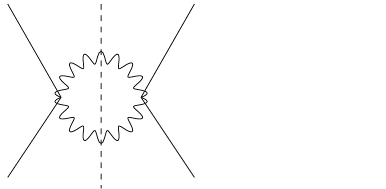
First we briefly review how unitarity survives in massless vector field theories. The requirement that the S-matrix is unitary implies that the scattering amplitude $T_{if}$ from the initial state $i$ to the final state $f$, defined as

$$S_{if}=\delta_{if}+i(2\pi)^{4}\delta(p_{i}-p_{f})T_{if},$$

(29)

satisfies the relation

$$T_{if}-T^{*}_{fi}=i\sum_{n}T_{in}T^{*}_{fn}(2\pi)^{4}\delta(p_{i}-p_{f}),$$

(30)

where the sum is taken over all physical states consistent with all conservation laws. The left hand side can be calculated purturbatively by means of the so-called Landau-Cutkosky rules [3]:

1. 1.

   Cut through the diagram in all possible ways such that the cut propagators can simultaneously be put on shell.

2. 2.

   Replace $1/(p^{2}+m^{2}+i\epsilon)$ by $-2\pi i\delta(p^{2}+m^{2})$ for each cut propagator, then perform the loop integrals.

3. 3.

   Sum over the contributions of all possible cuts.

Using these rules, it is possible to check unitarity order by order in a perturbation theory. For example, Fig. 3 shows three possible ways of the interaction $\phi\phi\rightarrow\phi\phi$ of order $O(e^{4})$. The Landau-Cutkosky rules include the replacement of the photon propagator in each internal line

$$\Delta_{\mu\nu}=\frac{g_{\mu\nu}-(1-\xi)\frac{k_{\mu}k_{\nu}}{k^{2}}}{k^{2}+i\epsilon}\rightarrow-2\pi i\left[g_{\mu\nu}-(1-\xi)\frac{k_{\mu}k_{\nu}}{k^{2}}\right]\delta(k^{2})\equiv-2\pi iG_{\mu\nu}\delta(k^{2}).$$

(31)

Therefore the left-hand side of (30) is

$$\mathrm{Im}\mathit{T}=M^{\mu\rho}G_{\mu\nu}G_{\rho\xi}M^{\nu\xi},$$

(32)

where $M^{\mu\rho}$ is an on-shell amplitude of $\phi\phi\rightarrow AA$ which contains three diagrams (Fig. 4.).

On the right-hand side of (30), the two diagrams obtained from cutting a diagram in Fig. (3) are multiplied. A cut vector internal line becomes two vector external lines in the two diagrams of the $\phi\phi\rightarrow AA$ process. The summation over polarizations of a pair of vector external lines contributes the factor

$$\sum_{\lambda=1,2}\epsilon^{*}_{\mu}(\lambda,k)\epsilon_{\nu}(\lambda,k)\equiv-E_{\mu\nu}.$$

(33)

The sum only includes physical polarizations, so

$$E_{\mu\nu}=g_{\mu\nu}-\frac{k_{\mu}n_{\nu}+k_{\nu}n_{\mu}}{n\cdot k}+\frac{n^{2}k_{\mu}k_{\nu}}{(k\cdot n)^{2}},$$

(34)

where $n_{\nu}$ is an arbitrary vector satisfying

$$k\cdot n\neq 0,\qquad n\cdot\epsilon(\lambda,k)=0,$$

(35)

Compare (31) and (34). Their difference is that the unphysical polarizations are included in $G_{\mu\nu}$ but not in $E_{\mu\nu}$. However, in ordinary QED there is no problem due to the fact that photons always couple to conserved currents

$$k_{\mu}M^{\mu\nu}=0.$$

(36)

Therefore,

$$M^{\mu\rho}G_{\mu\nu}G_{\rho\xi}M^{\nu\xi}=M^{\mu\rho}E_{\mu\nu}E_{\rho\xi}M^{\nu\xi}=M^{\mu\rho}g_{\mu\nu}g_{\rho\xi}M^{\nu\xi}$$

(37)

and unitarity is preserved.

In massive vector theories, the Ward-identity (36) no longer applies. Yet the situation is actually simpler. The sum over physical polarizations is

$$\sum_{\lambda=1,2,3}\epsilon_{\mu}(\lambda,k)\epsilon^{*}_{\nu}(\lambda,k)=g_{\mu\nu}+\frac{k_{\mu}k_{\nu}}{M^{2}},$$

(38)

which is exactly the numerator of the massive vector boson propagator. It means that there is no unphysical polarizations in the internal lines. In massive theories, the number of physical polarizations is three, and it is exactly the number of degrees of freedom of spin-one particles. On the other hand, for a massless vector field, in order to obtain a well-defined propagator, one introduces a gauge-fixing term of the form

$$\frac{-1}{2\xi}\Bigl(\partial_{\mu}A^{\mu}\Bigr)^{2}.$$

(39)

In the propagator the number of polarizations is 4, but there are only 2 physical polarizations. Therefore, we need Ward-identities to ensure that unphysical intermediate states decouple.

A well known theory containing massive vector bosons is the intermediate vector boson (IVB) model of weak interaction. In this theory heavy vector bosons $W^{\pm}$ are introduced to tame the high energy behavior of beta decay in Fermi’s four-fermion current-current model. But diagrams with external $W^{\pm}$ bosons [5, 6],

e.g. Fig. 5, still suffer high energy divergence. At the leading order, the cross section is [5, 6]

$$\frac{d\sigma}{d\Omega}=\frac{\sum_{pol}|M_{t}|^{2}}{64\pi^{2}s}\simeq\frac{G^{2}E^{2}\sin^{2}\theta}{8\pi^{2}}.$$

(40)

When the energy is large enough, the total probability of the scattering is larger than 1, and unitarity is violated, in a sense different from our discussions above.

The murderer of unitarity here is the longitudinal mode of $W^{\pm}$ bosons. Recall the polarization sum (38). The second term in (38), which results in bad high-energy behaviors, comes from the longitudinal mode.

To cancel this $E^{2}$ term, destructive interference in s-channel (Fig 6) and/or u-channel (Fig 6) is a possible way out. This motivated the introduction of the Z boson.

In our theory, we will also rely on the destructive interference among diagrams with the same external legs. For example, the pair annihilation $\phi^{+}_{n}\phi^{-}_{n}\rightarrow A_{a}A_{b}$ contains three diagrams at the tree level (Fig. 7),

the amplitude is

$$\mathcal{T}=-\frac{e_{n}^{2}}{c_{n}}\left[\frac{4(p_{1}\cdot\epsilon_{1})(p_{2}\cdot\epsilon_{2})}{m_{n}^{2}-t}+\frac{4(p_{1}\cdot\epsilon_{2})(p_{2}\cdot\epsilon_{1})}{m_{n}^{2}-u}+2(\epsilon_{1}\cdot\epsilon_{2})\right],$$

(41)

where

$$t=-(-p_{1}-k_{1})^{2},\qquad\mbox{and}\qquad u=-(-p_{1}-k_{2})^{2}.$$

(42)

Here the incoming momenta are defined to have negative energy and the relation of energy momentum conservation is

$$p_{1}+p_{2}+k_{1}+k_{2}=0.$$

(43)

Because we only worry about the $E^{4}$ term in $\mathcal{|T|}^{2}$, we focus our attention on leading order terms in the expansion

	$\displaystyle\frac{1}{m_{n}^{2}-t}$	$\displaystyle=\frac{1}{m_{n}^{2}+(p_{1}+k_{1})^{2}}=\frac{1}{2(p_{1}\cdot k_{1})-M_{a}^{2}}=\frac{1}{2p_{1}\cdot k_{1}}[1+\mathcal{O}(1/E^{2})],$		(44a)
	$\displaystyle\frac{1}{m_{n}^{2}-u}$	$\displaystyle=\frac{1}{m_{n}^{2}+(p_{1}+k_{2})^{2}}=\frac{1}{2(p_{1}\cdot k_{2})-M_{b}^{2}}=\frac{1}{2p_{1}\cdot k_{2}}[1+\mathcal{O}(1/E^{2})],$		(44b)

and the longitudinal polarizations are

$$\epsilon^{\mu}_{1}\rightarrow\frac{k_{1}^{\mu}}{M_{a}},\qquad\epsilon^{\mu}_{2}\rightarrow\frac{k_{2}^{\mu}}{M_{b}}.$$

(45a)

Using these relations, the high energy behavior of the amplitude in (41) is largely simplified

$$\mathcal{T}\rightarrow-\frac{e_{n}^{2}}{c_{n}}\left[\frac{2(p_{2}\cdot k_{2})}{M_{a}M_{b}}+\frac{2(p_{2}\cdot k_{1})}{M_{a}M_{b}}+2\frac{(k_{1}\cdot k_{2})}{M_{a}M_{b}}\right]=\frac{-e_{n}^{2}}{c_{n}}\frac{M_{a}^{2}+M_{b}^{2}}{M_{a}M_{b}}.$$

(46)

The term of order $E^{2}$ is suppressed due to the identity

$$s+t+u=2m_{n}^{2}+M_{a}^{2}+M_{b}^{2}.$$

(47)

We see in (46) the destructive interference among three diagrams. Unitarity is safe at high energies.

Next we consider the $\phi^{+}_{m}\phi^{-}_{m}\rightarrow\phi^{+}_{n}\phi^{-}_{n}$ diagram (Fig. 8).

The amplitude is

$$\mathcal{M}_{mmnn}=-ie_{m}(p_{1}-p_{2})^{\mu}\sum_{a}\frac{b_{a}(g_{\mu\nu}+\frac{(p_{1}+p_{2})_{\mu}(p_{3}+p_{4})_{\nu}}{M_{a}^{2}})}{M_{a}^{2}-s}(-ie_{n})(p_{3}-p_{4})^{\nu}.$$

(48)

Although the term $k^{\mu}k^{\nu}/M^{2}$ in the propagator leads to a term of 4th order in energy, it vanishes because

$$(p_{1}-p_{2})^{\mu}(p_{1}+p_{2})_{\mu}(p_{3}+p_{4})_{\nu}(p_{3}-p_{4})^{\nu}=(p_{1}^{2}-p_{2}^{2})(p_{3}^{2}-p_{4}^{2})=0.$$

(49)

Instead of imposing the equation of motion on (48), there is another way to control the $k^{\mu}k^{\nu}$ term in propagator. Take the $1/E$ expansion of (48),

$$\mathcal{M}_{mmnn}=-ie_{m}(p_{1}-p_{2})^{\mu}\sum_{a}\left[-b_{a}\frac{(p_{1}+p_{2})_{\mu}(p_{3}+p_{4})_{\nu}}{M_{a}^{2}\,s}+\mathcal{O}(1/E^{2})\right](-ie_{n})(p_{3}-p_{4})^{\nu},$$

(50)

the leading order term vanishes if the condition

$$\sum_{a=1}\frac{b_{a}}{M_{a}^{2}}=0$$

(51)

is imposed. Although this is not necessary here, we will meet the same condition in the next subsection in order for certain loop diagrams to be finite.

In general, the potential violation of unitarity at high energies due to massive vector bosons has its origin in the $k_{\mu}k_{\nu}/M^{2}_{a}$ term in the propagator. The same term is also responsible for potential nonrenormalizability. Our basic idea is to fine-tune the parameters $b_{a},M_{a}^{2}$ to achieve destructive interference among all massive vector bosons, such that the vector propagator is sufficiently well-behaved at high energies for the theory to be UV-finite and unitary.

In this subsection we calculate some one-loop diagrams, and show that UV divergences are canceled in every diagram if certain conditions on the parameters of the theory are matched. Then we discuss the cancellation in generic Feynman diagrams.

References

- [1] Pei-Ming Ho and Yi-Ya Tian, UV-finite scalar field theory with unitarity, [hep-th/0410248v2]
- [2] Pei-Ming Ho and Xue-Yan Lin, A UV completion of scalar field theory in arbitrary even dimensions , Journal of High Energy Physics, Springer Berlin / Heidelberg, 10.1007/JHEP01(2010)032 pp1-15. [hep-th/0910.3287v1]
- [3] R.E. Cutkosky, “Singularities And Discontinuities Of Feynman Amplitudes,” J. Math. Phys. 1, 429 (1960)
- [4] N. Itzhaki, Some interesting properties f field theories with an infinite number of fields, Int. J. Mod. Phys. A 13, 625 (1998)
- [5] Aitchison, I.J.R. , Hey, A.J.G.(1982), Gauge Theories in Particle Physics, Adam Hilger.
- [6] Gastmans R. 1975 Weak and Electromagnetic Interactions at High Energies, Cargese, 1975 ed M Levy et al (New York: Plenum) pp 109ff.
- [7] Cornwall, John M. and Levin, David N. and Tiktopoulos, George, Derivation of gauge invariance from high-energy unitarity bounds on the matrix, PhysRevD.10.1145, 1974
- [8] C.H. Llewellyn Smith, Phys. Letters 46B, 233, 1973
- [9] M.E. Peskin, D.V. Schroeder, An Introduction to Quantum Field Theory, Addison-Wesley Advanced Book Program(now Perseus Books) (1995)
- [10] Stefan Pokorsky, Gauge Field Theories, 2nd Edition, page 140-143, Cambridge Monographs on Mathematical Physics (1999)