Application of the DRA method to the calculation of the four-loop QED-type tadpoles.

The calculation of the high-order radiative corrections have become necessary in many areas of physics, from solid state physics to quantum electrodynamics (QED) and quantum chromodynamics (QCD). The radiative corrections are expressed in terms of the loop integrals, therefore it is necessary to be able to calculate them. Several powerful approaches to this problem have been developed. One of the most successful approach is based on the integration-by-parts (IBP) reduction procedure [1, 2]. This method allows one to reduce the problem of calculation of arbitrary loop integral to that of some finite set of master integrals. The important feature of the IBP reduction is that it may also help in the calculation of the master integrals. Namely, using the reduction one can obtain the differential [3, 4, 5, 6] and difference [7, 8] equations for the master integrals. Recently, in Ref. [9], the method of calculation based on the dimensional recurrence relation [7] and analyticity with respect to space-time dimensionality $\mathcal{D}$ (the DRA method) was suggested. This method was applied to the calculation of master integrals for several physical problems [10, 11, 12, 13]. In these papers the DRA method was combined with other methods such as the method of Mellin-Barnes representation [14] and sector decomposition method, implemented in FIESTA [15].

In the present paper we apply the DRA method to the calculation of the ‘QED-type’ four-loop master integrals depicted in Fig.1.

These integrals were considered in many papers, see Refs. [16, 17, 18, 19, 20, 21, 22, 23, 24, 25, 9, 12] and references therein. The numerical results for their $\epsilon$-expansions around $\mathcal{D}=4$ were obtained in Ref. [19] using Laporta’s difference equation method [8]. Some of the integrals are known in analytic form in terms of the hypergeometric function. The integrals $J_{6,3}$ and $J_{8,1}$ have been already investigated using DRA method, see Refs. [25, 9, 12]. For the majority of the integrals, several terms of the $\epsilon$-expansion around $\mathcal{D}=3$ and $\mathcal{D}=4$ were found in analytical form in Refs. [19, 20, 24]. However, the complete set of the analytical results for all integrals was not obtained so far. In particular, there is no analytical results for the $\epsilon$-expansion of the most complicated non-planar integral $J_{9,1}$ around $\mathcal{D}=3$. The goal of the present paper is twofold. First, we demonstrate some peculiarities of the application of the DRA method appearing in the calculation of the integrals considered. Second, we present the complete set of the analytical formulas for the $\epsilon$-expansions of the integrals in Fig.1 around $\mathcal{D}=3$ and $\mathcal{D}=4$.

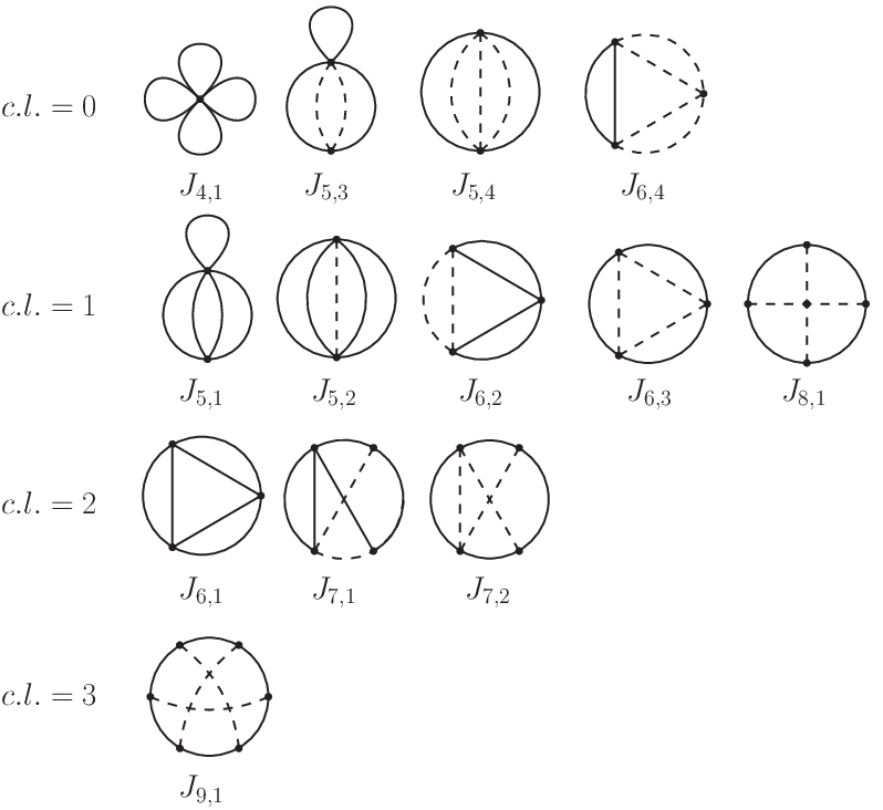
In order to calculate the integrals depicted in Fig.1, we use the DRA method [9], based on the dimensional recurrence relation and analytical properties of loop integrals as functions of $\mathcal{D}$. We evaluate integrals in the order determined by their complexity level [10], starting from $c.l.=1$ and ending with $c.l.=3$. The calculation of the integrals $J_{7,1}(\mathcal{D})$ and $J_{7,2}(\mathcal{D})$ demands a slight extension of the approach of Ref. [9], we demonstrate it by presenting here the calculation of the integral $J_{7,1}(\mathcal{D})$. Due to the chosen order of calculation, all simpler master integrals of $J_{7,1}(\mathcal{D})$ (the ones obtained by contracting some lines of $J_{7,1}(\mathcal{D})$) are already known at this stage.

Obviously, the integral $J_{7,1}(\mathcal{D})$ has no infrared divergences for $\mathcal{D}>2$. Similarly, it has no ultraviolet divergences for $\mathcal{D}<7/2$. Therefore, the integral is a holomorphic function in the stripe $\{\mathcal{D}|\,\mathrm{Re}\mathcal{D}\in(2,7/2)\}$. However, this stripe is too narrow to be chosen as a basic stripe of the DRA method. As it was pointed out in Ref. [9], in this case one can pass to a new master integral with dots on the massive lines in order to improve the ultraviolet behavior. A suitable choice is the integral $J_{7,1}^{a}(\mathcal{D})$ depicted in Fig. 2.

The integral $J_{7,1}^{a}(\mathcal{D})$ has no infrared divergences for $\mathcal{D}>2$, and no ultraviolet divergences for $\mathcal{D}<9/2$, thus, being a holomorphic function in the stripe $\{\mathcal{D}|\,\mathrm{Re}\mathcal{D}\in(2,9/2)\}$. Due to the IBP identities, the integral $J_{7,1}(\mathcal{D})$ can be expressed via $J_{7,1}^{a}(\mathcal{D})$ and simpler integrals as

$\displaystyle J_{7,1}(\mathcal{D})$

$\displaystyle=$

$\displaystyle G(\mathcal{D})+H(\mathcal{D})=\frac{8(2\mathcal{D}-9)}{3(\mathcal{D}-4)^{2}(3\mathcal{D}-10)}J_{7,1}^{a}(\mathcal{D})+H(\mathcal{D})\,,$

(1)

where $H(\mathcal{D})$ is the linear combination of the integrals $J_{4,1}(\mathcal{D})$, $J_{5,1}(\mathcal{D})$, $J_{5,2}(\mathcal{D})$, $J_{5,3}(\mathcal{D})$, $J_{6,2}(\mathcal{D})$, see Appendix. Therefore, we can apply the DRA method to the calculation of $J_{7,1}^{a}(\mathcal{D})$, and then use Eq. (1) to determine $J_{7,1}(\mathcal{D})$. However, we find it convenient to apply the DRA method directly to the integral $J_{7,1}(\mathcal{D})$, using Eq. (1) for the determination of the analytical properties of this integral in the basic stripe $S=\{\mathcal{D}|\,\mathrm{Re}\mathcal{D}\in(2,4]\}$. The singularities of $J_{7,1}(\mathcal{D})$ in $S$ are determined by those of two terms in the right hand side of Eq. (1). The singularities of the function $H(\mathcal{D})$ are located at $\mathcal{D}=10/3,\,7/2,\,4$ and totally fixed by the explicit form of the simpler master integrals (already calculated at this stage). The only singularities of the first term are the first- and the second-order poles at $\mathcal{D}=10/3$ and $\mathcal{D}=4$, respectively. The principal parts of the Laurent series expansion of the first term around these two points are not known. However, by the proper choice of summing factor $\Sigma(\mathcal{D})$ we can achieve that the product $\Sigma(\mathcal{D})G(\mathcal{D})$ is holomorphic in $S$, see below.

The dimensional recurrence relation for the integral $J_{7,1}(\mathcal{D})$ reads

$\displaystyle J_{7,1}(\mathcal{D}+2)$

$\displaystyle=$

$\displaystyle-\frac{64(2\mathcal{D}-7)(2\mathcal{D}-5)}{3(\mathcal{D}-2)^{2}(\mathcal{D}-1)\mathcal{D}(3\mathcal{D}-8)(3\mathcal{D}-4)}J_{7,1}(\mathcal{D})+R(\mathcal{D})\,,$

(2)

where the function $R(\mathcal{D})$ is given in the Appendix. Choosing the summing factor $\Sigma(\mathcal{D})$ in the form

$\displaystyle\Sigma({\mathcal{D}})=\frac{2^{7-2\mathcal{D}}\Gamma\left(\frac{9}{2}-\mathcal{D}\right)\Gamma\left(\frac{\mathcal{D}}{2}\right)}{\pi^{5/2}\Gamma\left(5-\frac{3\mathcal{D}}{2}\right)\Gamma(3-\mathcal{D})}\,,$

(3)

we can rewrite Eq. (2) as

$\displaystyle g(\mathcal{D}+2)=g(\mathcal{D})+r(\mathcal{D})\,,$

(4)

where $g(\mathcal{D})=\Sigma(\mathcal{D})J_{7,1}(\mathcal{D})$, $r(\mathcal{D})=\Sigma(\mathcal{D}+2)R(\mathcal{D})$. It follows from Eq. (3), that the function $\Sigma(\mathcal{D})$ has first-order zeros at $\mathcal{D}=3,\,10/3$, second-order zero at $\mathcal{D}=4$, and behaves at $\mathrm{Im}\mathcal{D}\to\pm\infty$ as $\exp\{\pi|\mathcal{D}|/2\}$. Therefore, the product $\Sigma(\mathcal{D})G(\mathcal{D})$ is a holomorphic function in $S$ and falls off exponentially at $\mathrm{Im}\mathcal{D}\to\pm\infty$. Our choice of $\Sigma(\mathcal{D})$ provides that the function $g(\mathcal{D})$ has only known singularities in $S$, and falls off exponentially at $\mathrm{Im}\mathcal{D}\to\pm\infty$. In order to represent the general solution of Eq. (4) in terms of infinite series, see Ref. [9], we need to decompose the function $r(\mathcal{D})$ as

$\displaystyle r(\mathcal{D})=r_{+}(\mathcal{D})+r_{-}(\mathcal{D}+2)\,,$

(5)

where $r_{\pm}(\mathcal{D}\pm 2k)$ decreases faster then $1/k$ at $k\to\infty$. However, the terms in $r(\mathcal{D})$, proportional to $J_{6,2}(\mathcal{D})$ and $J_{5,3}(\mathcal{D})$, decrease as $1/k$ at $k\to\infty$, and the decomposition (5) is not possible. In order to deal with this problem we use the following trick. Let us consider the dimensional recurrence relation

$\displaystyle\tilde{g}(\mathcal{D}+2)$

$\displaystyle=$

$\displaystyle\tilde{g}(\mathcal{D})+\tilde{r}(\mathcal{D})\,,$

(6)

for the linear combination

$$\tilde{g}(\mathcal{D})=\Sigma(\mathcal{D})\left(J_{7,1}(\mathcal{D})+\alpha(\mathcal{D})J_{6,2}(\mathcal{D})+\beta(\mathcal{D})J_{5,3}(\mathcal{D})\right)\,,$$

(7)

and try to find the rational functions $\alpha(\mathcal{D})$, $\beta(\mathcal{D})$ such that the terms proportional to $J_{6,2}(\mathcal{D})$ and $J_{5,3}(\mathcal{D})$ in $\tilde{r}(\mathcal{D})$ decrease faster than $1/k$ at large $k$. Using the explicit form of $\tilde{r}(\mathcal{D})$, see Appendix, we choose $\alpha(\mathcal{D})=-1$, and conclude that there is no proper choice of $\beta(\mathcal{D})$, and we simply put $\beta(\mathcal{D})=0$. After this, the function $\tilde{r}(\mathcal{D})$ can be presented as

	$\displaystyle\tilde{r}(\mathcal{D})$	$\displaystyle=$	$\displaystyle\tilde{r}_{+}(\mathcal{D})+\tilde{r}_{-}(\mathcal{D}+2)+\tilde{r}_{0}(\mathcal{D})\,,$		(8)
	$\displaystyle\tilde{r}_{0}(\mathcal{D})$	$\displaystyle=$	$\displaystyle-\frac{1}{\sin^{2}\left(\pi\mathcal{D}/2\right)}\frac{2}{\mathcal{D}}\,,$		(9)

where $\tilde{r}_{\pm}(\mathcal{D}\pm 2k)$ decrease faster then $1/k$ at $k\to\infty$. The function $\tilde{r}_{0}(\mathcal{D})$ corresponds to the large-$\mathcal{D}$ asymptotic of the term proportional $J_{5,3}(\mathcal{D})$ in $\tilde{r}(\mathcal{D})$. Obviously, $\tilde{r}_{0}(\mathcal{D}\pm 2k)\sim 1/k$ at large $k$, so that the sum

$\displaystyle\sum_{k=0}^{\infty}\tilde{r}_{0}(\mathcal{D}\pm 2k)$

(10)

diverges. Fortunately, the solution of Eq. (6) with $\tilde{r}$ replaced by $\tilde{r}_{0}$ can be written explicitly as

$$\tilde{g}_{0}(\mathcal{D})=-\frac{1}{\sin^{2}(\pi\mathcal{D}/2)}\psi\left(\frac{\mathcal{D}}{2}\right)\,,$$

(11)

where $\psi(x)=\Gamma^{\prime}(x)/\Gamma(x)$. Therefore, the general solution of the dimensional recurrence relation (6) has the form

$\displaystyle\tilde{g}(\mathcal{D})=\omega(z)-\sum_{k=0}^{\infty}\tilde{r}_{+}(\mathcal{D}+2k)+\sum_{k=0}^{\infty}\tilde{r}_{-}(\mathcal{D}-2k)+\tilde{g}_{0}(\mathcal{D})\,,$

(12)

where $\omega(z)=\omega\left(\exp[i\pi\mathcal{D}]\right)$ is arbitrary periodic function. It follows from Eq. (12) that the analytical properties of the function $\omega(z)$ are determined by those of $\tilde{g}$, $\tilde{r}_{\pm}$, and $\tilde{g}_{0}$. Namely, $\omega(z)$ is a meromorphic function, which has poles at $z=\pm i\,,\,\pm 1$, and falls off at $|z|\to\infty$. Since the principal parts of the Laurent series expansions around these points are determined by known integrals only, and not by $J_{7,1}$, the function $\omega(z)$ can be easily found (for brevity, we do not present its explicit form here). Finally, using Eqs. (4), (7), and (12) we obtain

$\displaystyle J_{7,1}(\mathcal{D})=J_{6,2}(\mathcal{D})+\Sigma^{-1}(\mathcal{D})\left(\omega(\mathcal{D})-\sum_{k=0}^{\infty}\tilde{r}_{+}(\mathcal{D}+2k)+\sum_{k=0}^{\infty}\tilde{r}_{-}(\mathcal{D}-2k)-\frac{1}{\sin^{2}(\pi\mathcal{D}/2)}\psi\left(\frac{\mathcal{D}}{2}\right)\right)\,.$

(13)

This equation is valid for arbitrary $\mathcal{D}$, and, in particular, can be used for the numerical calculation of $\epsilon$-expansion of $J_{7,1}(\mathcal{D})$ around $\mathcal{D}=3,\,4$. In two following sections we present such expansions for all integrals, depicted in Fig.1 The analytical form of the expansions is obtained from the high-precision numerical results using PSLQ algorithm Ref. [26], as implemented in MPFUN multiple-precision subroutines [27]. The coefficients in the expansions are expressed in terms of the following transcendental numbers:

$\displaystyle\zeta_{n}=\sum_{k=1}^{\infty}\frac{1}{k^{n}}\,,\quad a_{n}=\sum_{k=1}^{\infty}\frac{1}{2^{k}k^{n}}=\mathrm{Li}_{n}(1/2)\,,\quad s_{6}=\sum_{m=1}^{\infty}\sum_{k=1}^{m}\frac{(-1)^{m+k}}{m^{5}k}=0.98744\ldots$

(14)