Supersymmetric type-III seesaw:
lepton flavour violating decays and dark matter

In the case of seesaw type-I one postulates very heavy right-handed neutrinos yielding the following superpotential below $M_{GUT}$:

where $A\cdot B=A_{1}B_{2}-A_{2}B_{1}$ denotes the $SU(2)$ invariant product of two $SU(2)$ doublets. This model can be embedded in an $SU(5)$ using the following $SU(5)$ matter representations: $1=N^{c}$, ${\bar{5}}_{M}=\{D^{c},L\}$ and $10_{M}=\{Q,U^{c},E^{c}\}$. For the neutrino mass matrix one obtains the well-known formula

Being complex symmetric, the light Majorana neutrino mass matrix in eq. (5), is diagonalized by a unitary $3\times 3$ matrix $U$ [11]

Inverting the seesaw equation, eq. (5), allows to express $Y_{\nu}$ as [49]

where the $\hat{m}_{\nu}$ and $\hat{M}_{R}$ are diagonal matrices containing the corresponding eigenvalues. $R$ is in general a complex orthogonal matrix. Note that, in the special case $R={\bf 1}$, $Y_{\nu}$ contains only “diagonal” products $\sqrt{M_{i}m_{i}}$. For $U$ we will use the standard form

with $c_{ij}=\cos\theta_{ij}$ and $s_{ij}=\sin\theta_{ij}$. The angles $\theta_{12}$, $\theta_{13}$ and $\theta_{23}$ are the solar neutrino angle, the reactor (or CHOOZ) angle and the atmospheric neutrino mixing angle, respectively. $\delta$ is the Dirac phase and $\alpha_{i}$ are Majorana phases. In the following we will set the latter to 0 and consider in case of $\delta$ only the cases $0$ and $\pi$.

In seesaw models of type-II one adds a scalar $SU(2)$ triplet $T$ to generate neutrino masses. As this triplet carries also hypercharge one has to embed it in a $15$-plet of $SU(5)$ which has under $SU(3)\times SU(2)\times U(1)$ the following decomposition [14]

One has to add two 15-plets $15$ and $\overline{15}$ to avoid a chiral anomaly below the GUT-scale. The $SU(5)$ invariant superpotential reads as

with ${5}_{H}=(H^{c},H_{u})$ and ${\bar{5}}_{H}=({\bar{H}}^{c},H_{d})$. We do not show the part responsible for the $SU(5)$ breaking as we take the $SU(5)$ only as a guideline to fix some of the boundary conditions at $M_{GUT}$. Below $M_{GUT}$ in the $SU(5)$-broken phase the superpotential reads

where fields with index 1 (2) originate from the $15$-plet ($\overline{15}$-plet). The second term in eq. (17) is responsible for the generation of the neutrino masses yielding

Note that

i.e. $Y_{T}$ is diagonalized by the same matrix as $m_{\nu}$. If all neutrino eigenvalues, angles and phases were known, $Y_{T}$ would be fixed up to an overall constant which can be easily estimated to be

In addition there are the couplings $Y_{S}$ and $Y_{Z}$, which, in principle, are not determined by any low-energy data. In the calculation of LFV observables in supersymmetry both matrices, $Y_{T}$ and $Y_{Z}$, contribute. Having a GUT model in mind we require for the numerical discussion later the $SU(5)$ boundary conditions, apart from threshold corrections, $Y_{T}=Y_{S}=Y_{Z}$ at $M_{GUT}$.

As long as $M_{Z}\sim M_{S}\sim M_{T}\sim M_{15}$ gauge coupling unification will be maintained. The equality need not be exact for successful unification. In our numerical studies we have taken into account the different running of these mass parameters but we decouple them all at the scale $M_{T}(M_{T})$ because the differences are small.

In the case of a seesaw model type-III one needs new fermions $\Sigma$ at the high scale belonging to the adjoint representation of $SU(2)$. This has to be embedded in a 24-plet to obtain a complete $SU(5)$ representation. The superpotential of the unbroken $SU(5)$ relevant for our discussion is

As above, we have not specified the Higgs sector responsible for the $SU(5)$ breaking. The new parts, which will give the seesaw mechanism, comes from the $24_{M}$. It decomposes under $SU(3)\times SU(2)\times U(1)$ as

The fermionic components of $(1,1,0)$ and $(1,3,0)$ have exactly the same quantum numbers as $\nu^{c}$ and $\Sigma$. Thus, the $24_{M}$ always produces a combination of the type-I and type-III seesaw.

In the $SU(5)$ broken phase the superpotential becomes

As before we use at the GUT scale the boundary condition $Y_{N}=Y_{B}=Y_{X}$ and $M_{B}=M_{G}=M_{W}=M_{X}$. Integrating out the heavy fields yields the following formula for the neutrino masses at the low scale:

As mentioned above there are two contributions stemming from the gauge singlet as well as from the $SU(2)$ triplet. In this case the calculation of the Yukawa couplings in terms of a given high scale spectrum is more complicated than in the other two types of seesaw models. However, as we start from universal couplings and masses at $M_{GUT}$ we find that at the seesaw scale one still has $M_{B}\simeq M_{W}$ and $Y_{B}\simeq Y_{W}$ so that one can write in a good approximation

and one can use the corresponding decomposition for $Y_{W}$ as discussed in section II.1 up to the overall factor $4/5$.

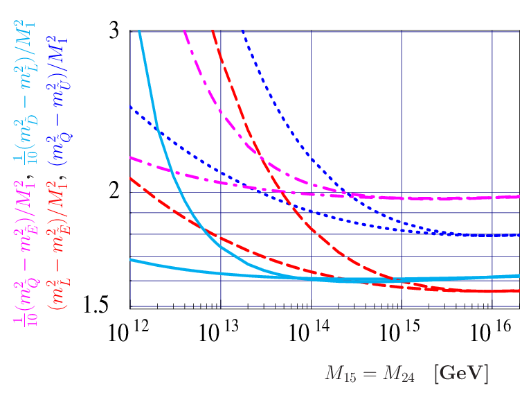
The appearance of charged particles at scales between the electro-weak scale and the GUT scale leads to changes in the beta functions of the gauge couplings [14, 15]. In the MSSM the corresponding values at 1-loop level are $(b_{1},b_{2},b_{3})=(33/5,1,-3)$. In case of one 15-plet the additional contribution is $\Delta b_{i}=7/2$ whereas in case of 24-plet it is $\Delta b_{i}=5$. This results in case of type-II in a total shift of $\Delta b_{i}=7$ for the minimal model and in case of type-III in $\Delta b_{i}=15$ assuming 3 generations of 24-plets. This does not only change the evolution of the gauge couplings but also the evolution of the gaugino and scalar mass parameters with profound implications on the spectrum [15, 28]. Additional effects on the spectrum of the scalars can be present if some of the Yukawa couplings get large [28, 50, 29] which can also happen in type-I models [51]. In Fig. 1 we exemplify this by showing the values of selected mass parameters at $Q=1$ TeV versus the seesaw scale for fixed high scale parameters $m_{0}=M_{1/2}=1$ TeV and we have set the additional Yukawa couplings to zero. As expected, the effects in case of models of type-II and III are larger the smaller the corresponding seesaw-scale is. The scalar mass parameters shown are of the first generation and, thus, the results are nearly independent of $\tan\beta$ and $A_{0}$. For illustration we show in Fig. 2 the corresponding spectrum where we have fixed $\tan\beta=10$ and $A_{0}=0$.

We note that in all three model types the ratio of the gaugino mass parameters is nearly the same as in the usual mSUGRA scenarios but the ratios of the sfermion mass parameters change [15, 28]. One can form four ’invariants’ for which at least at the 1-loop level the dependence on $M_{1/2}$ and $m_{0}$ is rather weak, e.g. $(m^{2}_{L}-m^{2}_{E})/M^{2}_{1}$, $(m^{2}_{Q}-m^{2}_{E})/M^{2}_{1}$, $(m^{2}_{D}-m^{2}_{L})/M^{2}_{1}$ and $(m^{2}_{Q}-m^{2}_{U})/M^{2}_{1}$. Here one could replace $M_{1}$ by any of the other two gaugino masses which simply would amount in an overall rescaling. In Fig. 3 we show these ’invariants’ in the leading-log approximation at 1-loop order to demonstrate the principal behaviour for seesaw type-II with a pair of ${\bf 15}$-plets and seesaw type-III with three ${\bf 24}$-plets. From this one concludes that in principle one has a handle to obtain information on the seesaw scale for given assumptions on the underlying neutrino mass model, if universal boundary conditions are assumed. For the type-I, i.e. singlets only, of course $\Delta b_{i}=0$ and no change with respect to mSUGRA are expected. If, for example, the seesaw III model would be realized in nature with three 24-plets having similar masses around $10^{13}$ GeV one could e.g. show that the corresponding ratios cannot be obtained with one pair of 15-plets in the seesaw II model, thus excluding this possibility. However, taking the seesaw II with two pairs of 15-plets one would obtain similar ratios as in this case the corresponding additional beta-functions at 1-loop would be $\Delta b_{i}=14$, e.g. nearly equal to our seesaw III model.

The leading-log approximation gives only the general trend, but there is an important dependence on the SUSY point chosen. In Fig. 4 we show as illustration $(m^{2}_{L}-m^{2}_{E})/M^{2}_{1}$ and $(m^{2}_{Q}-m^{2}_{E})/M^{2}_{1}$ for different mSUGRA points and at different loop orders: the dashed lines are at 1-loop level whereas the solid ones are at 2-loop level. The points considered are SPS3 [52] with $m_{0}=90$ GeV, $M_{1/2}=400$ GeV, $A_{0}=0$, $\tan\beta=10$, $\mu>0$ and for the same values of $A_{0}$ and $\tan\beta$ two points with $M_{1/2}=1$ TeV: $m_{0}=500$ GeV and $m_{0}=1$ TeV. The black line shows for comparison the leading-log approximation. We observe that usually the approximation gets worse for lower values of $M_{24}$ and this is even stronger at the 2-loop level which is a consequence of the large coefficient in the beta functions at the 2-loop level, see e.g. appendix A.4. Nevertheless, one sees that in general it gives the correct trend, but it might even fail completely, e.g. in the case of $M_{1/2}=m_{0}=1$ TeV. The reason for the drop around $M_{24}\simeq 3.5\times 10^{13}$ is that the difference between the parameters goes to zero as can also be seen from the right of Fig. 1, see also discussion below.

Last but not least we note that the use of the 2-loop RGEs leads to a shift of $M_{GUT}$ from about 2$\times 10^{16}$ GeV for 24-plet mass of $10^{16}$ GeV to about 4$\times 10^{16}$ GeV for 24-plet mass of $10^{13}$ GeV, which is part of the differences between the 1-loop and 2-loop results in Fig. 4. Here $M_{GUT}$ is defined as the scale where the electro-weak couplings meet, e.g. $g_{U(1)}=g_{SU(2)}$. This implies also that there is some difference for the strong coupling which is, however, in the order of 5-10% which can easily be accounted for by threshold effects of the new GUT particles, e.g. the missing members of the gauge fields and the Higgs fields responsible for the breaking of the GUT group [53]. A second reason why the deviations between the leading log calculation, the case of 1-loop and 2-loop RGEs gets larger for smaller seesaw scale is that the increase of the beta coefficients implies larger values of the gauge couplings at the GUT scale. This implies that one reaches a Landau pole for sufficiently low values of the seesaw scale. As an example we show in Fig. 5 the value of the gauge coupling at $M_{GUT}=2\times 10^{16}$ GeV as a function of the seesaw scale for type-II with a pair of 15-plets (black lines) and type-III with three degenerate 24-plets (green lines). In both cases the 2-loop RGEs imply a larger gauge coupling for a fixed seesaw scale. One sees that in case of type-II (type-III) in principle one could reach a seesaw scale of about $10^{8}$ GeV ($10^{13}$ GeV). However, we believe that we can no longer trust even the 2-loop calculation for such large values of the $g_{i}$, as the neglected higher order terms become more and more important. Especially, we should not trust the “turn-over” of the invariants in Fig. 4 for very low values of the seesaw scale, since the numerical calculation at these points is already very close to breaking down.

We would also like to mention that, in the numerical calculation we find very often that one of the scalar masses squared, in particular staus and/or sbottoms, gets large negative values already for values of the seesaw scale larger than the Landau pole and thus we can not go to values of the seesaw scale as low as the examples shown in Fig. 4 in many SUSY points.

>From a one-step integration of the RGEs one gets assuming mSUGRA boundary conditions a first rough estimate for the lepton flavour violating entries in the slepton mass parameters:

for $i\neq j$ in the basis where $Y_{e}$ is diagonal, $L_{ij}=\ln(M_{GUT}/M_{i})\delta_{ij}$ and $Y^{k}_{N}$ is the additional Yukawa coupling of the type-$k$ seesaw at $M_{GUT}$ ($k=I,II,III$). We obtain

Note, that in case of the type-II the matrix $L$ is degenerate and thus can be factored out. All models have in common that they predict negligible flavour violation for the right-sleptons

We know that these approximations work well only in case of the type-I models. Nevertheless they give a rough idea on the relative size one has to expect for the rare lepton decays $l_{i}\to l_{j}\gamma$ which very roughly scale like

where $\widetilde{m}$ is the average of the SUSY masses involved in the loops. Note, that for a given set of high scale parameters both, the different size of the flavour mixing entries and the changed mass spectrum, play a role.

We have seen in eq. (30) that rates for the lepton flavour violating decays of $\mu$ and $\tau$ scale like the LFV entries in the slepton mass squared matrix squared and inverse to the overall SUSY mass to the power eight. From this one immediately concludes the rates for the rare lepton decays are in general larger in seesaw models of type-II and III than in type-I models for fixed SUSY masses and seesaw scales except if one arranges for special cancellations.

Comparing the type-II with the type-III model one finds that LFV decays are larger for type-III, as shown for the case of $\mu\to e\gamma$ in Fig. 6. From eqs. (27) and (28), however, one would expect that type-II should have larger LFV. Numerically we find the opposite for two reasons. (i) $Br(l_{i}\to l_{j}\gamma)$ strongly depends on the SUSY masses, see eq. (30) and type-III has a lighter spectrum than type-II (for the same mSUGRA input parameters). And (ii) 2-loop effects are very important in type-III, due to the large coefficients, in general leading to large flavor violating soft SUSY breaking parameters.

In Fig. 6 we compare $Br(l_{i}\to l_{j}\gamma)$ for the three seesaw models taking degenerate seesaw spectra in case of type-I and type-III. Note that in case of seesaw type-III we can only show a relatively short interval for the seesaw scale which is mainly due to two reasons: (i) for scales below approximately $10^{13}$ GeV the gauge couplings get large at $M_{GUT}$ as a consequence of the large beta functions and, thus, perturbation theory breaks down. (ii) One encounters negative mass squares for the scalars, in particular for the lighter stau and/or lighter sbottom. The latter point is also the reason why the possible range is larger in case of the larger soft SUSY breaking parameters.

The values for $Br(\mu\to e\gamma)$ in Fig. 6 are larger than the current experimental bound [58], so one might worry if in case of type-III models only SUSY spectra beyond the reach of the LHC are allowed. (Note, that even for the examples shown the masses of the sfermions are already in the range of several hundred GeVs as can be seen from table 1.) Indeed we find that by putting generic Yukawa couplings which are able to explain neutrino data one needs a heavy spectrum to be consistent with bounds on the rare lepton decays. However, this is strictly true only for the TBM angles and $R=$1. Accidental cancellations due to different contributions to the flavor violating soft masses and thus to the rare lepton decays are possible in type-III (and in type-I). As an example we show in Fig. 7 $Br(\mu\to e\gamma)$ as a function of the reactor angle $s^{2}_{13}$ for different values of the Dirac phase $\delta$. For comparison we also show the calculation for a type-I model. For $\delta=\pi$ there is a range of $s^{2}_{13}$ where this branching ratio is below the experimental constraint.

At first glance this seem to require some fine-tuning of the underlying parameters. However, one can look at this from a different perspective: Assume that the MEG collaboration has found a non-vanishing value for $Br(\mu\to e\gamma)$ and from LHC data one has found that the spectrum is consistent with the type-III seesaw model. For a fixed $R$-matrix, e.g. $R$=1 one would obtain in this case a relation between $s^{2}_{13}$ and $M_{24}$. This can be exploited to put a bound on $M_{24}$ or even to determine it depending on the outcome of measurements of reactor angle and, thus, the model assumptions can be tested. In Fig. 8 we show the corresponding rare tau decays. Note that also for $\tau\to e\gamma$ such a cancellation exists in principle but the corresponding range is excluded by $\mu\to e\gamma$. In contrast $\tau\to\mu\gamma$ is insensitive to the reactor angle and should be measurable in the near future.

Up to now we have assumed that the seesaw spectrum is nearly degenerate which is of course a strong assumption. We show in Fig. 9 two examples where we keep in each case two masses fixed and vary the third one. Note, that in contrast to SUSY particles the indices of the heavy particles are generation indices and do not correspond to a particular mass ordering, e.g. $M_{R_{2}}$ corresponds to the ’solar neutrino scale’ and $M_{R_{3}}$ to the ’atmospheric neutrino scale’. In case that the mass of the first generation state is varied, e.g. the left plot of this figure, one finds a decrease of the branching ratios with increasing seesaw mass $M_{R_{1}}$. This is mainly caused by an increase of the SUSY spectrum while at the same time neutrino physics is only affected mildly requiring only a light increase of the corresponding Yukawa couplings to obtain the correct neutrino masses. If, on the other hand, the mass $M_{R_{3}}$ of the third generation seesaw particles is increased on needs also a sizable increase of the Yukawa couplings to obtain the correct neutrino mass difference squared for the atmospheric sector. This leads to the observed behaviour that the branching ratios for $\tau\to\mu\gamma$ and $\tau\to 3\mu$ increases while the other ones decrease.

The changes in the spectrum induced by the new heavy states also impact on the predictions with respect to the relic density which we have calculated using the program micrOMEGAs [59]. As is well-known, within mSUGRA there are 4 regions in parameter space, in which the constraint from dark matter can be satisfied. These are (i) the bulk region; (ii) the stau co-annihilation region; (iii) the focus point line and (iv) the Higgs funnel. Below we will show usually the range of $\Omega h^{2}$ allowed at 3 $\sigma$ according to [58]

In particular, the co-annihilation region is very sensitive to the difference between the masses of the lightest stau and the lightest neutralino. In Fig. 10 we observe that this difference depends strongly on the seesaw scale in both models. For a fixed $M_{1/2}$ and $m_{0}$ lowering the seesaw scale increases this mass difference, which then leads to a larger calculated $\Omega h^{2}$. To compensate for this effect one needs to lower $m_{0}$, with the value depending on the seesaw scale chosen. For certain seesaw scales then $m_{0}$ needs to be lowered below $m_{0}=0$ and the co-annihilation region disappears. In this region of parameter space both models behave in a qualitatively similar way. However, recall that spectra run faster towards smaller masses in seesaw type-III.

Also the focus point region is very sensitive to the precise values of the input parameters. The focus point region appears in mSUGRA for large values of $m_{0}$ and small/moderate values of $M_{1/2}$ of the order of ${\cal O}(100)$ GeV, the exact value depending on $m_{0}$. This can be seen in figs. 11 and 12 where we show $m_{\tilde{\chi}^{0}_{1}}$, the higgsino content $|N_{13}|^{2}+|N_{14}|^{2}$ and the corresponding $\Omega h^{2}$ as a function of $m_{0}$ for a fixed seesaw scale $M_{T,W}=10^{14}$ GeV, $A_{0}=0$, $\tan\beta=10$, $\mu>0$ and various values of $M_{1/2}$. Note, that we take different values of $M_{1/2}$ for the two models in such a way that we obtain similar values for $m_{\tilde{\chi}^{0}_{1}}$. We find that both models behave differently in this region of parameter space, e.g. the higgsino content $|N_{13}|^{2}+|N_{14}|^{2}$ decreases (increases) with increasing values $m_{0}$ for seesaw type-II (type-III). However, also for type-II the higgsino content increases for increasing $m_{0}$ once we reach the multi-TeV range but we did not get correct electroweak symmetry breaking in case of multi-TeV values for $m_{0}$ in case of type-III models. The increased higgsino content of the lightest neutralino leads to on increase (decrease) of its couplings to the $Z$-boson and the light Higgs boson (to sfermions) resulting in the observed dependence of $\Omega h^{2}$ for $m_{0}$ close to the 1-TeV region.

With these observations it is clear that the DM allowed regions will be shifted in the $m_{0}$-$M_{1/2}$ plane compared to the usual mSUGRA expectations. We fix in the following $m_{top}=171.2$ GeV, $\tan\beta=10$, $A_{0}=0$ and $\mu>0$ as well as the seesaw scale to $10^{14}$ GeV. For comparison we show in Fig. 13 the usual mSUGRA case without any heavy intermediate particles (left plot) as well as the case of a seesaw type-I scenario (right plot). The blue bands show the 3$\sigma$ range according to [58] and we see the three usual regions: the stau co-annihilation with a lighter stau mass close to the LSP mass for $M_{1/2}\raise 1.29167pt\hbox{$\;<$\kern-7.5pt\raise-4.73611pt\hbox{$\sim\;$}}300$ GeV, the bulk region for moderate values of $M_{1/2}$ and $m_{0}$ resulting in small sfermion masses as well as the focus point region for $M_{1/2}\simeq$ 170 GeV and large values of $m_{0}$. In addition, we show the lines corresponding to $M_{h}=110$ GeV and 114 GeV. Note, that the theoretical uncertainty on $M_{h}$ is still of the order of 3-5 GeV [60, 61]. Moreover, the value of the Higgs boson mass also depends strongly on $A_{0}$ and in particular for negative values of $A_{0}$ one can easily increase the value of $M_{h}$ while the DM allowed regions hardly change.

The part of parameter space most affected is the one at large $m_{0}$. Since in mSUGRA $\mu$ is calculated from the requirement of correct electroweak symmetry breaking, $\mu$ changes rapidly in this region. With the Higgsino content in the lightest neutralino changing rapidly as a function of $\mu$, this region is then very sensitive to any changes of parameters. Since the $Y_{\nu}$ also impacts on the running of the Higgs mass parameters and thus slightly affects the value predicted for $\mu$, some small changes are found relative to mSUGRA here. Note, however, that this region is highly constrained by the lower bound on the lightest chargino mass of the order of 103 GeV [62].

In case of the other two seesaw models the shift of the allowed regions is much more pronounced, as discussed above. In Figs. 14 and 15 we show to regions for type-II (left plot) and type-III (right plot) and two different values for $A_{0}$. As claimed above, the Higgs mass bounds gets shifted significantly while the DM allowed regions are hardly affected. As expected the effects are much more pronounced in case of type-III as the effects of the heavy particles on the spectrum is much stronger. Note, that in particular the bending of the allowed region for large $m_{0}$ is due to the changed higgsino content as discussed in case of figs. 11 and 12. Moreover, the case of stau co-annihilation is not viable anymore in case of the type-III model already for this value of the seesaw scale. For completeness we mention that for the type-II the stau co-annihilation region disappears (below $M_{1/2}=1500$ GeV) for $M_{T}\raise 1.29167pt\hbox{$\;<$\kern-7.5pt\raise-4.73611pt\hbox{$\sim\;$}}10^{13}$ GeV. For completeness we note that the results here differ slightly from the ones of our previous work [42] because (i) of the corrections of the 1-loop RGEs of ref. [14] by [47] and (ii) the complete set of 2-loop RGEs are now used.

In the case of large $\tan\beta$ an additional region, usually called the Higgs funnel, opens up. This region is characterized by $M_{A}\simeq 2m_{\tilde{\chi}^{0}_{1}}$. Also here the regions gets shifted compared to usual mSUGRA scenario. However, this region is very sensitive to higher order corrections and therefore it is quite important to use full 2-loop RGEs as can be seen in Fig. 16. We have again fixed $A_{0}$ = 0, $\mu>0$, $m_{top}=171.2$ GeV and the seesaw scale to $10^{14}$ GeV, with a degenerate spectrum in case of the type-III model. The main reason for the observed and rather surprisingly large differences between the different calculations is that the 2-loop contributions decrease the neutralino mass compared to the 1-loop case while at the same time increasing $M_{A}$. For example, in case of seesaw II and for fixed values of $m_{0}=M_{1/2}$ = 1500 GeV we get in case of 1-loop RGEs $m_{\tilde{\chi}^{0}_{1}}=560$ GeV, $M_{A}=1090$ GeV and in case of 2-loop RGEs $m_{\tilde{\chi}^{0}_{1}}=498$ GeV, $M_{A}=1100$ GeV. For completeness we note that this region is also very sensitive to input values for $m_{t}$ and $m_{b}$ [42].

References

• [1] Y. Fukuda et al. [Super-Kamiokande Collaboration], Phys. Rev. Lett. 81, 1562 (1998)
• [2] SNO, Q. R. Ahmad et al., Phys. Rev. Lett. 89, 011301 (2002), [nucl-ex/0204008].
• [3] KamLAND, K. Eguchi et al., Phys. Rev. Lett. 90, 021802 (2003), [hep-ex/0212021].
• [4] KamLAND Collaboration, arXiv:0801.4589 [hep-ex].
• [5] T. Schwetz, M. A. Tortola and J. W. F. Valle, New J. Phys. 10, 113011 (2008) [arXiv:0808.2016 [hep-ph]]. Version 3 on the arXive is updated with data until Feb 2010
• [6] S. Weinberg, Phys. Rev. Lett. 43, 1566 (1979); S. Weinberg, Phys. Rev. D 22, 1694 (1980).
• [7] E. Ma, Phys. Rev. Lett. 81, 1171 (1998) [arXiv:hep-ph/9805219].
• [8] P. Minkowski, Phys. Lett. B 67 (1977) 421.
• [9] T. Yanagida, in KEK lectures, ed. O. Sawada and A. Sugamoto, KEK, 1979; M Gell-Mann, P Ramond, R. Slansky, in Supergravity, ed. P. van Niewenhuizen and D. Freedman (North Holland, 1979);
• [10] R.N. Mohapatra and G. Senjanovic, Phys. Rev. Lett. 44 912 (1980).
• [11] J. Schechter and J. W. F. Valle, Phys. Rev. D 22, 2227 (1980).
• [12] T. P. Cheng and L. F. Li, Phys. Rev. D 22, 2860 (1980).
• [13] R. Foot, H. Lew, X. G. He and G. C. Joshi, Z. Phys. C 44, 441 (1989).
• [14] A. Rossi, Phys. Rev. D 66, 075003 (2002) [arXiv:hep-ph/0207006].
• [15] M. R. Buckley and H. Murayama, Phys. Rev. Lett. 97, 231801 (2006) [arXiv:hep-ph/0606088].
• [16] J. Hisano, T. Moroi, K. Tobe and M. Yamaguchi, Phys. Rev. D53, 2442 (1996), [hep-ph/9510309].
• [17] J. R. Ellis, J. Hisano, M. Raidal and Y. Shimizu, Phys. Rev. D 66, 115013 (2002) [arXiv:hep-ph/0206110].
• [18] F. Deppisch, H. Paes, A. Redelbach, R. Rückl and Y. Shimizu, Eur. Phys. J. C28, 365 (2003), [hep-ph/0206122].
• [19] S. T. Petcov, S. Profumo, Y. Takanishi and C. E. Yaguna, Nucl. Phys. B 676 (2004) 453 [arXiv:hep-ph/0306195].
• [20] E. Arganda and M. J. Herrero, Phys. Rev. D73, 055003 (2006), [hep-ph/0510405].
• [21] S. T. Petcov, T. Shindou and Y. Takanishi, Nucl. Phys. B 738, 219 (2006) [arXiv:hep-ph/0508243].
• [22] S. Antusch, E. Arganda, M. J. Herrero and A. M. Teixeira, JHEP 11, 090 (2006), [hep-ph/0607263].
• [23] F. Deppisch and J. W. F. Valle, Phys. Rev. D 72, 036001 (2005) [arXiv:hep-ph/0406040].
• [24] J. Hisano, T. Moroi, K. Tobe, M. Yamaguchi and T. Yanagida, Phys. Lett. B357, 579 (1995), [hep-ph/9501407].
• [25] M. Hirsch, J. W. F. Valle, W. Porod, J. C. Romao and A. Villanova del Moral, Phys. Rev. D 78, 013006 (2008) [arXiv:0804.4072 [hep-ph]].
• [26] E. Arganda, M. J. Herrero and A. M. Teixeira, JHEP 10, 104 (2007), [0707.2955].
• [27] F. Deppisch, T. S. Kosmas and J. W. F. Valle, Nucl. Phys. B752, 80 (2006), [hep-ph/0512360].
• [28] M. Hirsch, S. Kaneko and W. Porod, Phys. Rev. D 78, 093004 (2008) [arXiv:0806.3361 [hep-ph]].
• [29] C. Biggio and L. Calibbi, arXiv:1007.3750 [hep-ph].
• [30] J. Hisano, M. M. Nojiri, Y. Shimizu and M. Tanaka, Phys. Rev. D 60, 055008 (1999) [arXiv:hep-ph/9808410].
• [31] J. N. Esteves, J. C. Romao, A. Villanova del Moral, M. Hirsch, J. W. F. Valle and W. Porod, JHEP 0905, 003 (2009) [arXiv:0903.1408 [hep-ph]].
• [32] G. A. Blair, W. Porod and P. M. Zerwas, Eur. Phys. J. C27, 263 (2003), [hep-ph/0210058].
• [33] A. Freitas, W. Porod and P. M. Zerwas, Phys. Rev. D72, 115002 (2005), [hep-ph/0509056].
• [34] F. Deppisch, A. Freitas, W. Porod and P. M. Zerwas, 0712.0361.
• [35] B. C. Allanach, J. P. Conlon and C. G. Lester, Phys. Rev. D 77, 076006 (2008) [arXiv:0801.3666 [hep-ph]].
• [36] A. Abada, A. J. R. Figueiredo, J. C. Romao and A. M. Teixeira, arXiv:1007.4833 [hep-ph].
• [37] E. Komatsu et al., arXiv:1001.4538 [astro-ph.CO].
• [38] K. Griest and D. Seckel, Phys. Rev. D 43, 3191 (1991).
• [39] H. Baer, C. Balazs and A. Belyaev, JHEP 0203, 042 (2002) [arXiv:hep-ph/0202076].
• [40] J. L. Feng, K. T. Matchev and T. Moroi, Phys. Rev. D 61, 075005 (2000) [arXiv:hep-ph/9909334].
• [41] M. Drees and M. M. Nojiri, Phys. Rev. D 47, 376 (1993) [arXiv:hep-ph/9207234].
• [42] J. N. Esteves, S. Kaneko, J. C. Romao, M. Hirsch and W. Porod, Phys. Rev. D 80, 095003 (2009) [arXiv:0907.5090 [hep-ph]].
• [43] F. Staub, arXiv:0806.0538 [hep-ph].
• [44] F. Staub, Comput. Phys. Commun. 181, 1077 (2010) [arXiv:0909.2863 [hep-ph]].
• [45] F. Staub, arXiv:1002.0840 [Unknown].
• [46] S. P. Martin and M. T. Vaughn, Phys. Rev. D 50, 2282 (1994) [Erratum-ibid. D 78, 039903 (2008)] [arXiv:hep-ph/9311340].
• [47] F. Borzumati and T. Yamashita, arXiv:0903.2793 [hep-ph].
• [48] S. K. Kang, T. Morozumi and N. Yokozaki, arXiv:1005.1354 [hep-ph].
• [49] J. A. Casas and A. Ibarra, Nucl. Phys. B 618, 171 (2001) [arXiv:hep-ph/0103065].
• [50] L. Calibbi, M. Frigerio, S. Lavignac and A. Romanino, JHEP 0912 (2009) 057 [arXiv:0910.0377 [hep-ph]].
• [51] L. Calibbi, Y. Mambrini, S. K. Vempati, JHEP 0709 (2007) 081. [arXiv:0704.3518 [hep-ph]].
• [52] B. C. Allanach et al., in Proc. of the APS/DPF/DPB Summer Study on the Future of Particle Physics (Snowmass 2001) ed. N. Graf, Eur. Phys. J. C 25 (2002) 113 [arXiv:hep-ph/0202233].
• [53] W. Martens, L. Mihaila, J. Salomon and M. Steinhauser, arXiv:1008.3070 [hep-ph].
• [54] W. Porod, Comput. Phys. Commun. 153, 275 (2003) [arXiv:hep-ph/0301101].
• [55] For the latetst version of SPheno, see the web page: http://www.physik.uni-wuerzburg.de/ porod/SPheno.html
• [56] S. Antusch and M. Ratz, JHEP 0207, 059 (2002) [arXiv:hep-ph/0203027].
• [57] P. F. Harrison, D. H. Perkins and W. G. Scott, Phys. Lett. B 530, 167 (2002) [arXiv:hep-ph/0202074].
• [58] C. Amsler et al. [Particle Data Group], Phys. Lett. B 667, 1 (2008).
• [59] G. Belanger, F. Boudjema, A. Pukhov and A. Semenov, Comput. Phys. Commun. 176, 367 (2007) [arXiv:hep-ph/0607059].
• [60] B. C. Allanach, A. Djouadi, J. L. Kneur, W. Porod and P. Slavich, JHEP 0409, 044 (2004) [arXiv:hep-ph/0406166].
• [61] S. Heinemeyer, W. Hollik, H. Rzehak and G. Weiglein, Eur. Phys. J. C 39, 465 (2005) [arXiv:hep-ph/0411114].
• [62] LEPSUSYWG, ALEPH, DELPHI, L3 and OPAL experiments, note LEPSUSYWG/01-03.1 (http://lepsusy.web.cern.ch/lepsusy/Welcome.html).
• [63] I. Jack, D. R. T. Jones and A. Pickering, Phys. Lett. B 426, 73 (1998) [arXiv:hep-ph/9712542].
• [64] Y. Yamada, Phys. Rev. D 50 (1994) 3537 [arXiv:hep-ph/9401241].
• [65] P. C. West, Phys. Lett. B 137 (1984) 371.
• [66] D. R. T. Jones and L. Mezincescu, Phys. Lett. B 138, 293 (1984).
• [67] I. Jack, D. R. T. Jones, S. P. Martin, M. T. Vaughn and Y. Yamada, Phys. Rev. D 50 (1994) 5481 [arXiv:hep-ph/9407291].
• [68] I. Jack, D. R. T. Jones and A. Pickering, Phys. Lett. B 432 (1998) 114 [arXiv:hep-ph/9803405].
• [69] http://theorie.physik.uni-wuerzburg.de/ fnstaub/supplementary.html