Proposal for an optical laser producing light at half the Josephson frequency

Lasers and superconductors are both systems with macroscopic quantum coherence. In lasers, photons form a coherent state induced by stimulated emission of a driven system into a cavity mode. The resulting visible coherent light is characterized by an optical phase [1]. In superconductors, the ground state arising from spontaneous symmetry breaking is also characterized by a phase [2].

Traditionally, lasers and superconductors are studied separately. Recently [3], it has been realized that the superconducting (SC) phase difference and the optical phase may interact in a single device that combines two superconductors and a semiconducting p-n junction. The latter is a common system for light generation as the electron-hole recombination produces photons of visible frequency [4]. Combining semi- and superconductors within a nanostructure has been a difficult technological problem that attracted attention for a long time [5]. It has been solved using semiconductor nanowires [6] or quantum wells [7], opening up the possibility to make combined devices.

The device in question has been termed a Josephson LED [Fig. 1(a)]. It employs a double quantum dot (QD) in a p-n semiconductor nanowire connected to SC leads [3]. The device, biased with a voltage $V$, exhibits two types of photon emission: “blue” photons at the Josephson frequency $\omega_{J}=2eV/\hbar$ due to the recombination of a Cooper pair from each side of the junction, and “red” photons at about $\omega_{J}/2$ due to electron-hole recombination. It has been shown that the optical phase of the Josephson generated “blue” photons is locked with the SC phase difference. The resulting “blue” light could in principle be enhanced by traditional optical methods but its small intensity makes this a challenging task.

In this Letter, we explore an alternative idea where the far more intense “red” emission is enhanced in a resonant cavity mode. We find lasing at half the Josephson frequency and, thus, dub the device ‘Half-Josephson Laser’ (HJL). In a common laser, lasing results from spontaneous symmetry breaking where all values of the optical phase are equivalent. Drift between these values leads to a finite decoherence time. In contrast, the optical phase of the HJL is locked to the SC phase difference with only two allowed values of the optical phase corresponding to two opposite radiation amplitudes. This removes drift as a source of decoherence and opens up the possibility to manipulate the optical phase by changing the SC phase difference. Instead, decoherence of the radiation in the HJL results from switching between different QD states accompanied by the emission of a photon. We have explored these processes and find that by order of magnitude the resulting decoherence time is the same as the theoretical limit for a common laser $\tau_{{\rm dec}}=n/\Gamma$, with $\Gamma$ the damping rate and $n$ the number of photons accumulated in the resonant mode. A rather low $\Gamma$ is required to achieve lasing for a single Josephson LED, this condition being relaxed with a large number of LEDs in a single cavity [8].

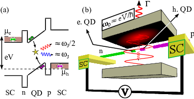
Setup and model The HJL is a Josephson LED embedded in a single mode optical cavity with resonance frequency $\omega_{0}\approx\tfrac{1}{2}\omega_{J}$, Fig. 1(b). The light emission from the cavity is described by a damping rate $\Gamma$. The electronic part consists of a biased p-n junction where each side of the junction accommodates a QD connected to a SC lead. The barriers separating the QDs from the leads are arranged such as to allow charge transfer only through electron-hole recombination. Such QD junctions can be realized with semiconducting nanowires [9].

The minimal model for the QDs involves a single orbital for each QD. An orbital can house up to two particles (including spin) yielding 16 possible states. The QD Hamiltonian then reads [10]

where $\hat{n}_{e}=\sum_{\sigma}\hat{c}^{\dagger}_{\sigma}\hat{c}^{\vphantom{\dagger}}_{\sigma}$ ($\hat{n}_{h}=\sum_{\sigma}\hat{h}^{\dagger}_{\sigma}\hat{h}^{\vphantom{\dagger}}_{\sigma}$) is the electron (hole) number operator, and $\hat{c}_{\sigma}$ ($\hat{h}_{\sigma}$) is the annihilation operator for an electron (hole) with spin $\sigma$. The energies $E_{e,h}$ are measured with respect to chemical potentials $\mu_{e,h}$ of the corresponding leads that differ by an energy $eV=\mu_{e}-\mu_{h}$; here, $U_{e,h}>0$ is the on-site charging energy and $U_{eh}<0$ the Coulomb attraction between electrons and holes. For concreteness, we assume that the hole level houses a heavy hole with $J_{z}=\pm\tfrac{3}{2}\hbar$, where $z$ is the nanowire axis [4, 11]. Such levels are commonly used in optical experiments with QDs [12]. Our qualitative results do not depend on this particular choice.

Due to the proximity of the SC leads, Cooper pairs can coherently tunnel between the SC leads and the QDs introducing mixing between unoccupied and doubly occupied QD states. These processes can be compactly described by an additional term $\hat{H}_{\scriptscriptstyle\rm SC}=\tilde{\Delta}_{e}^{*}\hat{c}_{\uparrow}\hat{c}_{\downarrow}+\tilde{\Delta}_{h}\hat{h}_{\uparrow}\hat{h}_{\downarrow}+\text{H.c.}$ in the Hamiltonian; here, the induced pair potentials $\tilde{\Delta}_{e,h}$ have reduced magnitudes in comparison with the gaps $\Delta_{e,h}$ of the SC leads but they retain the same phases $\phi_{e,h}$. Owing to gauge invariance, the physical quantities depend only on SC phase difference $\phi\equiv\phi_{e}-\phi_{h}$ The Hamiltonian is valid under the conditions $|\tilde{\Delta}_{e,h}|,E_{e,h},U_{e,h},U_{eh}\lesssim|\Delta|$. We note further that this Hamiltonian along with the electron-hole recombination conserves parity (even or odd) of the total number of particles on the QDs. Even-odd transitions require creation of quasiparticle excitations in the SC leads and occur with a relatively slow rate estimated below.

Interaction between the resonant mode and QDs is described by $\hat{H}_{\text{int}}=-{\bf E}\cdot{\bf\hat{d}}$; ${\bf E}$ being electric field of the mode at QD position and ${\bf\hat{d}}$ the dipole moment of the optical transition between the conduction and the valence band. We assume a linear polarized mode, choose the $x$-axis in the direction of the polarization, and notice that for heavy holes $\hat{d}_{x}\propto(\hat{x}e^{-ieVt/\hbar}+{\rm H.c.})$ with $\hat{x}\equiv(\hat{h}_{\downarrow}\hat{c}_{\uparrow}+\hat{h}_{\uparrow}\hat{c}_{\downarrow})$. The time-dependence of the dipole moment is due to the applied voltage. It is convenient to implement a rotating-wave approximation transferring the time-dependent factor to the photon creation (annihilation) operator $\hat{b}^{\dagger}$ ($\hat{b}$). Thereby, the photon-dependent part of the Hamiltonian reads

with $\omega$ being the frequency detuning, $\omega=\omega_{0}-eV/\hbar$, $|\omega|\ll\tfrac{1}{2}\omega_{J}$. We see that $\hat{x}$ plays the role of a driving force that excites the oscillations in the mode. We note that all Hamiltonians considered conserve spin.

Semiclassics The present model is a rather complex case of nonequilibrium dissipative quantum mechanics. However, since we envisage a large number of photons in the mode, we employ a semiclassical approximation replacing $\hat{b}\mapsto\langle\hat{b}\rangle\equiv\lambda/G$. The Hamiltonian $H_{\scriptscriptstyle\rm QD}+H_{\scriptscriptstyle\rm SC}+H_{\text{ph}}$ can then be diagonalized to obtain the spectrum $E_{m}(\lambda)$ and corresponding eigenstates $|m\rangle$. The dipole strength $x_{m}(\lambda)\equiv\langle m|\hat{x}|m\rangle$ depends both on the radiation field $\lambda$ and the QD state $|m\rangle$. Since the dipole strength in turn determines the evolution of the radiation field via the evolution equation

we have to solve the system self-consistently [1]. The radiation field can build up as long as the energy gain rate $2\hbar\omega_{0}(G^{2}/\hbar)\text{Im}[x_{m}(\lambda)/\lambda]$ due to the nanowire is greater than the energy loss rate $\hbar\omega_{0}\Gamma$. With increasing $\lambda$ the energy gain saturates till a stationary state of radiation (SSR) with $\dot{\lambda}=0$ is reached at a certain radiation amplitude $\lambda_{s}$.

In conventional lasers, the driving is due to a population inversion that originates from dissipative transitions in an open system. For the HJL, the SC drive is not dissipative by itself: only the emission of photons from the cavity is a dissipative process. The driving originates from coherent mixing of discrete quantum states due to the proximity of the QD to the SC leads without any population inversion. Thus, the driving mechanism of the HJL is very different from that of a conventional laser. This is why the information about the SC phase difference is preserved in the process of driving. The energy gain, including its sign, depends on the difference between $\phi$ and the phase of $\lambda$. Owing to this, the phase of $\lambda_{s}$ of the SSR is locked to the SC phase difference. The SSRs of the HJL come in pairs $\pm\lambda_{s}$ which is very different from a conventional laser where only the magnitude $|\lambda_{s}|$ (photon number) is fixed. We give in [8] analytical solutions to Eq. (3) for a toy two-level model.

Scales Let us estimate the scales involved that are expected to yield lasing. To simplify, we assume all characteristics of the QD spectrum to be of the same energy scale $E$ which is of the order $E\simeq|\tilde{\Delta}_{e,h}|\ll eV$. This assures optimal mixing of the QD states by superconductivity. In a lasing state, the radiation amplitude should noticeably contribute to the energies of the QD states. This requires $|\lambda|\simeq E$. Assuming $\omega\simeq\Gamma$ we estimate from Eq. (3) that this takes place at $G\simeq\sqrt{\hbar\Gamma E}$. We will assume that $G$ is always chosen to be of this scale. The number of photons is then estimated as $n\simeq|\lambda|^{2}/G^{2}\simeq E/\hbar\Gamma$. The semiclassical approximation is thus justified provided $\Gamma$ is sufficiently small, $\Gamma\ll E/\hbar$.

Lasing Despite the model being minimal, it contains ten parameters that affect the existence and characteristics of the SSRs. To find these characteristics, we need to evaluate the dipole moment in a given state at given $\lambda$, and can do it separately for the states of odd and even parity since they are not mixed by interactions. Additionally, the spin conservation splits the eight odd states into two equivalent groups of four corresponding to total spin $\pm\tfrac{1}{2}$. For the even states, only one of the four possible $|1_{e}1_{h}\rangle$ states, $(\hat{h}^{\dagger}_{\downarrow}\hat{c}^{\dagger}_{\uparrow}+\hat{h}^{\dagger}_{\uparrow}\hat{c}^{\dagger}_{\downarrow})|0\rangle$, couples to the field. Hence, we only need to consider five of the eight even states as the other three are dark.

With this, we demonstrate lasing as proof of concept by finding SSRs in the even states for QD parameters within the above estimated scales, $-E_{e}=E_{h}=\tfrac{1}{2}U_{e}=\tfrac{1}{2}U_{h}=-U_{eh}=\Delta_{h}\equiv E$ and $\Delta_{e}=1.5E$, for wide regions in the space of detuning $\omega$ and coupling $G$, see Fig. 2. Note that each eigenstate $|m\rangle$ has a different dipole strength $x_{m}$ such that the lasing threshold $G_{c}$ [Fig. 2(a)] and the radiation amplitudes of the SSRs $\lambda_{s}$ [Fig. 2(c) and (d)] depend on $m$. Figure 2(b) shows the number of photons upon crossing the lasing threshold for the state $|2\rangle$. In agreement with the estimations, $n$ reaches the maximum $\simeq E/\hbar\Gamma$ at $G\simeq\sqrt{\hbar\Gamma E}$. We stress that the optical phase of the radiation amplitude in an SSR is not arbitrary but locked to the SC phase difference [Fig. 2(c)].

Switching In the above discussion, we have assumed the QD to stay in a certain eigenstate $|m\rangle$. In fact it does not: the finite spectral width of the mode enables switching between the eigenstates. As shown below, the switching events occur on a much longer timescale $\Gamma^{-1}_{{\scriptscriptstyle\rm SW}}$ than that of the relaxation of $\lambda$ towards its stationary value, $\Gamma^{-1}$. This separation of timescales allows to consider the switching dynamics separately from the dynamics of the radiation amplitude.

Each switching event is accompanied by the emission of a photon with a frequency mismatch compensating the difference of energies between initial and final eigenstates, $\hbar\omega_{k}=E_{f}-E_{i}$. For switchings not altering the parity of the eigenstate, the rates $\Gamma_{\scriptscriptstyle\rm SW}$ can be evaluated using Fermi’s Golden Rule that contains the effective density of photon states $\Gamma/\hbar\omega_{k}^{2}$ (the tail of a Lorentzian-shaped emission line of the resonant mode) and the square of the matrix element, $|\langle m_{f}|\hat{H}_{\text{ph}}|m_{i}\rangle|^{2}$, with $|m_{i(f)}\rangle$ denoting the initial (final) state. Thereby, the switching rate can be estimated as $\Gamma_{\scriptscriptstyle\rm SW}\simeq\Gamma G^{2}/E^{2}\simeq\Gamma/n\ll\Gamma$. The switching events are thus rare and the device stays in one of the SSRs between the events.

Switchings altering parity are even rarer as they require the excitation of a quasi-particle above the SC energy gap $|\Delta_{e,h}|$. The larger detuning of the off-resonant photon $\omega_{k}\simeq|\Delta_{e,h}|/\hbar$ and an additional small factor $|\tilde{\Delta}_{e,h}/\Delta_{e,h}|$ result in a parametrically smaller rate $\Gamma_{\text{e-o}}\simeq|\tilde{\Delta}|\Gamma G^{2}/|\Delta|^{3}\ll\Gamma_{\scriptscriptstyle\rm SW}$ [3]. Such processes do not conserve spin thus enabling switchings between dark and emitting states.

It is important to realize that, since the SSRs for different eigenstates have different values of $\lambda_{s}^{m}$, $\lambda$ does not jump to the new stationary value upon a switching. Rather, the amplitude will evolve to $\lambda_{s}^{m_{f}}$ within a timescale $\simeq\Gamma^{-1}$ , according to Eq. (3). For the same reason a switching event always involves different eigenstates rather than different SSRs at the same eigenstate. The latter would require large fluctuations of $\lambda$ that are suppressed exponentially. Fig. 3 shows a sketch of the radiation intensity as function of time. In contrast to common lasers, the HJL intensity fluctuations are large at timescales of $\Gamma^{-1}_{{\scriptscriptstyle\rm SW}}$.

Decoherence The intrinsic mechanism of decoherence in common lasers is a drift of the optical phase. For the HJL, this mechanism does not work since the amplitudes of the SSRs are locked to the SC phase difference. This renders switching the most important source of decoherence in the HJL. Indeed, after switching from a lasing to a non-lasing SSR the radiation extinguishes quickly and its phase is forgotten. Even if the next switching brings the system to a lasing eigenstate, the radiation will evolve from the initial $\lambda=0$ to any of the two possible $\pm\lambda_{s}^{m}$, with equal probability. Since decoherence is due to switching, the relevant timescale is given by $\tau_{\text{dec}}\simeq\Gamma_{\scriptscriptstyle\rm SW}^{-1}\simeq n/\Gamma$. Despite the very different decoherence mechanism, this estimation is the same as for the common laser [13].

Average power and current The intensity fluctuations due to switching self-average at timescale exceeding $\Gamma_{{\scriptscriptstyle\rm e-o}}^{-1}$. The averaged characteristics are expressed in terms of the probabilities $P_{s}^{m}$ to be in a SSR $s$ that belongs to an eigenstate $|m\rangle$. Those are given by the stationary solution to the master equation of the switching dynamics, that is composed of the switching rates [8]. In terms of these probabilities, the average number of photons in the cavity is given by $\bar{n}=\sum_{m,s}P_{s}^{m}|\lambda_{s}^{m}|^{2}/G^{2}$. The average emission power is proportional to the photon number, $W=\tfrac{1}{2}\hbar\omega_{J}\Gamma\bar{n}$. The same holds for current in the device: since the emission of each photon is accompanied by a charge transfer, it is given by $I=e\Gamma\bar{n}=W/V$. An elaborated example of the current/intensity dependences is provided in [8]. For the current-voltage characteristic, we find a rather complex structure beside a peak with a magnitude of the order $eE/\hbar$, that is concentrated in a narrow interval $\simeq\hbar\Gamma/e$ of voltages in the vicinity $eV=\hbar\omega_{0}$. In this structure, two types of discontinuities are present: (i) kinks marking the thresholds of lasing instability at $\lambda=0$ (second-order transitions) and (ii) jumps signaling the appearance of a SSR with stationary radiation amplitude $\lambda_{s}$ far from $\lambda=0$ (first-order transitions). We observe a relatively high probability to remain in an SSR with a large photon number. It is explained from the fact that eigenstates at large $\lambda$ are close to eigenstates of $\hat{x}$. This suppresses off-diagonal dipole-matrix elements resulting in a suppressed rate of transitions from this state.

Feasibility To show the feasibility of the HJL, we present here the estimations with concrete numbers. The SC gaps $|\Delta_{e,h}|$ are typically $\simeq 1\,$meV, so we can choose the QD energy scale $E\simeq 0.1\,$meV. To estimate the dipole strength $G\simeq ea|\mathbf{E}_{0}|$ , with $|\mathbf{E}_{0}|\simeq\sqrt{\hbar\omega_{0}/\text{Vol}}$ being the quantum fluctuation of the electric field in the mode, we assume the cavity volume $\text{Vol}\simeq\ell^{3}$ with the wavelength $\ell=2\pi c/\omega_{0}\simeq 600\,\text{nm}$, and take $a\simeq 5\,$Å for the atomic distance scale. This gives the maximum $G\simeq 0.1\,$meV.

With these two values for $E$ and $G$, the minimum damping rate required for lasing is $\Gamma\simeq G^{2}/\hbar E\simeq 10^{11}\,$Hz, corresponding to quality factor $Q\simeq 10^{3}$ which is common for optical cavities. However, in this situation the number of photons $n\simeq 1$. This can be enhanced by increasing $Q$ and simultaneous decreasing $G$ so it remains $\simeq\sqrt{\hbar\Gamma E}$. For photonic crystal cavities [14] quality factors $Q\simeq 10^{6}$ [15] have been measured and $Q\simeq 10^{8}$ [16] have been theoretically predicted. This gives photon numbers $n\simeq 10^{3}$ and $n\simeq 10^{5}$, respectively. The estimations of the emitted power and current at the peak do not depend on the choice of $\Gamma$ and are given by $W\simeq 10\,$nW, $I\simeq 10\,$nA. The requirements on $\Gamma$ can be eased and $n$ enhanced by putting many Josephson LEDs in the same cavity. Furthermore, this also increases the emission power $W$ and the current $I$ [8].

In conclusion, we have demonstrated the feasibility of generating coherent visible light at half the Josephson frequency in a SC nanodevice. The workings of the device resemble the spontaneous parametric down-conversion in nonlinear optics [17] with the superconductors playing the role of coherent optical input. The novel driving mechanism results in locking between optical phase and SC phase difference. The decoherence of the emitted light originates from the switchings between different quantum states of the device.