Effect of topology on the critical charge in graphene
Abstract
We show that the critical charge for the Dirac excitations in gapless graphene depends on the spatial topology of the sample. In particular, for graphene cones, the effective value of the critical charge can tend towards zero for a suitable angle of the conical sample. We discuss the nature of the scattering phase shifts, quasi-bound state energies and local density of states for a gapless graphene cone and determine the dependence of these physical quantities on the sample topology.
I Introduction
The fabrication of monolayer graphene [1, 2, 3] provides an opportunity to study the effect of sample topology on its electronic properties [4, 5, 6, 7, 8, 9]. The low energy excitations of the gapless graphene are described by a two dimensional massless Dirac equation [10, 11, 12, 13, 14]. These excitations are negatively charged and behave like electrons with the Fermi velocity . In graphene, even a small external charge impurity can produce strong nonperturbative effects, since the effective Coulomb interaction strength , where the dielectric constant . Thus, graphene provides an ideal system to analyze the combined effects of topology and strong electric fields on its electronic properties.
The idea of a critical charge plays an interesting role in this context [15, 16, 17, 19, 18]. It is well known that massless Dirac fermions can tunnel through large external potentials, thereby avoiding trapping or formation of bound states. This phenomenon, known as Klein tunneling [21, 22, 20, 23, 24], is possible in graphene due to the chiral nature of the Dirac excitations [18, 20]. However, when the effective strength of the external charge exceeds a certain critical value , the low energy excitations can form quasi-bound states [15, 16, 17, 19, 18]. For such states the wavefunctions oscillate rapidly near the position of the charge impurity, analogous to zitterbewegung in strong field QED [25, 24]. For planar graphene, the critical charge . The existence of such quasi-bound states and their effect on transport properties and local density of states (LDOS) in planar graphene have attracted considerable attention [15, 16, 17, 18].
In this paper we explore how a nontrivial topology of the sample may affect the critical charge and the corresponding strong field QED effects in graphene. We address this issue for graphene cones, which are obtained by introducing local defects in the hexagonal lattice structure, for example, in the form of a pentagonal ring [4, 5]. The conical topology manifests itself in the form of nontrivial holonomies for the pseudoparticle wavefunctions. Such holonomies can be modelled through the introduction of a magnetic flux tube. Thus an electric charge localized at the apex of the cone can be equivalently described by a suitable combination of electric charge and magnetic flux tube. We show that the critical charge depends on the angle of the graphene cone. For certain angle of the graphene cone, the topological effects lead to the identification of the two Fermi points [4, 5]. This leads to the surprising conclusion that for a certain value of the angle of the cone, the critical charge is zero. We discuss the effect of the conical topology on the scattering phase shifts, quasi-bound state energies and local density of states (LDOS) in graphene.
This paper is organized as follows. In the next Section we set up the Dirac equation for gapless graphene cone with a point charge at the apex. This is followed by the analysis of the corresponding spectrum, where we obtain the scattering phase shits, quasi-bound state energies and local density of states (LDOS) and show how these physical quantities depend explicitly on the sample topology. We also briefly comment on the RG flow of the strength of the charge impurity. We end this paper with some discussion and outlook.
II Dirac equation for a graphene cone with a Coulomb charge
In this section we set up the Dirac equation for a graphene cone with a coulomb charge at the apex of the cone. The low energy properties of the quasiparticle states near the Dirac points in graphene can be described by the four component Dirac wave function [10, 11, 12] given by
The pseudospin indices and label the two sublattices of the primitive cell of graphene and the valley indices and label the two inequivalent Dirac points and respectively.
Considering low energy excitations about the Dirac point , Dirac equation for a planar gapless graphene in the presence of a Coulomb charge is given by
| (8) |
where is the radial coordinate in the two dimensional plane. The Pauli matrices and the identity matrix act on the pseudospin indices. The Coulomb interaction strength . From now on we set . In a two dimensional plane, the angular boundary condition for a Dirac spinor as it goes around a closed path is given by
| (9) |
A cone is obtained from the two dimensional plane by introducing a topological defect, which modifies the angular boundary condition (9). Following [4], consider a cone, formed by removing the sector (see Fig.1a.) and then identifying the edge , labeled by with the edge , labeled by . The sector subtends an angle at the centre . Due to this identification the frame becomes discontinuous across the joining line. This problem can be solved by choosing a new set of frames given by
| (10) |
which is rotated with respect to old frame by an angle in the counter clockwise direction, see Fig.1b. To keep the form of the Hamiltonian the same, the wave function has to be transformed by . Similarly, if sectors are removed from the plane where can take only discrete values , the wave function should be transformed as
| (11) |
Note that an additional negative sign appears in the boundary condition since we take the angular part of the wavefunction to be , being a half integer [4, 5].


When n is odd, an additional phase change is required due to the breaking of the bipartite nature of the hexagonal lattice. It can be seen from the Fig.(2), that the removal of a wedge of opening angle introduces a pentagonal defect. When the cone is formed by removing a single wedge of angle , the adjacent points on two sides of the identification line belong to the same sublattice. This feature is valid for all allowed odd and leads to a system with only one Fermi point. Considering all the factors, the angular boundary condition satisfied for a general value of is given by [4, 5].
| (12) |
Here acts on the valley indices . Note that for , the angular boundary condition for the planar graphene is recovered. For the allowed even values of and , it can be seen from (12) that the matrix plays no role in the angular boundary condition [4, 5]. This is due to the fact that for even , . For odd , the two Dirac points are identified and the energy eigenstates of the Dirac equation are obtained by diagonalizing which mixes the valley indices in the wavefunction [4, 5]. Since the eigenvalues of are , for all values of , we can replace the angular boundary condition (12) by
| (13) |
In subsequent analysis, we shall use the form (13) of the angular boundary condition assuming that for all allowed odd values of , the matrix acting on the valley indices has already been diagonalized.
The effect of the angular boundary condition (13) on the wave function can be equivalently described by introducing a magnetic flux tube passing through the apex of the cone [4]. The presence of a magnetic vector potential modifies the boundary condition on a Dirac spinor as
| (14) |
Taking as a line element on the circumference of the cone at a distance from the apex, we have
| (15) |
Substituting (15) in (14) and assuming that is independent of the angle , we get
| (16) |
Comparing equation (13) and equation (16) we get
| (17) |
Thus the entire effect of the conical topology on the wavefunction can be described by introducing the vector potential (10), which replaces the ordinary derivatives by the corresponding covariant derivatives in the Hamiltonian (8). In this effective description, the Hamiltonian for a graphene cone with a Coulomb charge at the apex is given by
| (18) |
where the relation between and can be obtained from the Equation(10), which gives and and . Thus the Dirac equation (8) can be written as
We use an ansatz for the wavefunction given by
where the total angular momentum takes all half integer values. Substituting (II) in (II), we note that the leading short distance behaviour of the wavefunction is given by
| (31) |
From (31) it follows that when exceeds , becomes imaginary. As a result, the eigenstates and becomes wildly oscillatory and have no well defined limit as , which corresponds to the phenomenon of zitterbewegung in a strong Coulomb electric field [25]. The critical value of the coupling is denoted by and it is given by the minimum allowed value of . The parameter depends on and the number of sectors removed from a plane to form the graphene cone. Hence we see that the critical coupling explicitly depends on the angle of the graphene cone. The values of the critical charge for different values of n are given in TABLE 1.
| value of | Critical charge | Corresponding angular momentum |
| 0 | ||
| 1 | 0.3 | |
| 2 | 0 | |
| 3 | 0.5 | |
| 4 | 1.5 | |
| 5 | 1.5 |
From these values of critical charge, a surprising result can be observed for the case of , where is zero. In this case, any external charge will be supercritical.We should also note that when , none of the values of in the lowest angular momentum channel , corresponds to the minimum value of or the critical charge. In this case the critical charge of the system is obtained from the angular momentum channel .
III Spectrum in graphene cone with a supercritical charge
In this Section we derive the scattering and bound state spectra for a gapless graphene cone in the presence of a supercritical Coulomb charge located at the apex of the cone. First consider the case . Using (II) and (II), the Dirac equation in each angular momentum channel can be written as
In terms of the functions and defined by and , we get
| (37) |
and
| (38) |
| (39) |
where , with . For the discussion below, for any given value of and , we choose greater than the corresponding value of . This ensures that the coupling is always in the supercritical region. Define where . Then the solution of Eq.(39) is given by
| (40) |
| (41) |
where .
In order to proceed, we use the zigzag edge boundary condition , where is a distance from the apex, of the order of the lattice scale in graphene [16]. This gives
| (42) |
From the above, we obtain the scattering matrix as
| (43) |
where . From (43) we obtain the scattering phase as
| (44) |
where . In Fig. (3a) we plot (44) ignoring the Coulomb tail term . For , the value of is deeper in the supercritical region than it is for . When the coupling is deeper in the supercritical region, the phase shift has more number of kinks, which indicate the bound states. The plot also shows that the phase shift depends on the topology through its dependence on via .
 |
 |
As mentioned before, in gapless graphene we do not expect bound states due to Klein tunneling. However, in the supercritical regime, the system admits quasi-bound states whose spectrum is obtained from the zeroes of the matrix in (43). The quasi-bound state energies are given by
| (45) |
where is a positive integer.
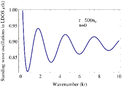
Another interesting observable in this context is the LDOS. In Fig.(4) we have plotted the standing wave oscillations in LDOS using
| (46) |
where is the radial part of the spinor given in Eq.(II), for a given angular momentum channel .
 |
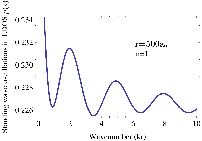 |
The maxima and minima of the oscillations occur at half-integral and integral multiple of respectively. The normalization constant of the wave function depends on the value of which decreases with increasing . Therefore, though the nature of standing wave oscillation is similar for and , the amplitudes of the corresponding LDOS decreases with the increase of .
It is known that in the planar case, under the RG flow, a supercritical charge is driven to its critical value [16]. While the full discussion of the RG flow requires a more detailed analysis, we can obtain some of its qualitative features from the quasi-bound state energies. To see this consider the real part of in (45) which gives the energy. This part diverges as the cutoff . In order to study the RG flow, we now promote the coupling constant as a function of and demand that as , the energy for any fixed level (say ) remains independent of the cutoff [26, 27]. In the leading order, where is only slightly above the critical coupling, this prescription gives the -function as
| (47) |
Thus we have an ultraviolet stable fixed point at or at . Hence, for any given value of and , the coupling in the supercritical regime is driven to its critical value.
We end this Section with a comment for the case , which occurs for and . For , the first order Dirac equations (37) and (38) completely decouple and the functions and become independent of each other. In this case, the critical coupling also vanishes. This means that any external charge, no matter how small, would lead to the supercritical regime.
IV Conclusion
In this paper we use the fact that system of a graphene cone with an external Coulomb charge at its apex can be equivalently described by the combination of the Coulomb charge and a suitable magnetic flux tube passing through the apex. The above analysis has been done in the supercritical regime, where the external Coulomb charge exceeds a certain critical value.
The quantities of physical interest in this system include the scattering phase shifts, the LDOS and the quasi-bound state energies. We have shown that all these physical quantities depend explicitly on the number of sectors removed from a planar graphene to form the cone. The existence of the quasi-bound states indicates the possibility of the localization of the wavefunctions in the presence of a supercritical charge. Our analysis shows that the nature and extent of the localization depends on the spatial topology of the graphene sample.
Finally, we have given qualitative arguments which shows that under the RG flow and for , the supercritical charge in the graphene cone tends to its critical value. If this argument can be extended for , for which the critical charge vanishes, that would lead to complete shielding of the external charge. This issue and the related electronic properties are currently under investigation.
References
- [1] K. S. Novoselov, A. K. Geim, S. V. Morozov, D. Jiang, M. I. Katsnelson, I. V. Grigorieva and A. A. Firsov, Science 306, 666 (2004).
- [2] K. S. Novoselov, A. K. Geim, S. V. Morozov, D. Jiang, M. I. Katsnelson, I. V. Grigorieva, S. V. Dubonos and A. A. Firsov, Nature 438, 197 (2005).
- [3] Y. Zhang, Y.-W. Tan, H. L. Stormer and P. Kim, Nature 438, 201 (2005).
- [4] P.E. Lammert, V.H. Crespi, Phys. Rev. Lett. 85, 5190 (2000).
- [5] P.E. Lammert, V.H. Crespi, Phys. B 69, 035406 (2004).
- [6] D. V. Kolesnikov and V. A. Osipov, Eur. Phys. J. B 49, 465 (2006).
- [7] A.Cortijo, M.A.H.Vozmediano, Nucl. Phys. B 763, 293 (2007).
- [8] C.Furtado, F.Moraes, A.M. de M. Carvalho, Phys. Lett. A 372, 5368 (2008).
- [9] A. Roy and M. Stone, J. Phys. A 43, 015203 (2010).
- [10] Wallace, P. R. The band theory of graphite. Phys. Rev. 71, 622–634 (1947).
- [11] A. K. Geim and K.S. Novoselov, Nature Materials 6, 183-191 (2007).
- [12] A.H.Castro Neto, F.Guinea, N.M.R. Peres, K.S. Novoselov and A.K.Geim, Rev. Mod. Phys. 81, 109 (2009).
- [13] D. P. DiVincenzo and E. J. Mele, Phys. rev. B 29, 1685 (1984).
- [14] G. W. Semenoff, Phys. Rev. Lett. 53, 2449 (1984).
- [15] V. M. Pereira, J. Nilsson and A. H. Castro Neto, Phys. Rev. Lett. 99, 166802 (2007).
- [16] A. V. Shytov, M. I. Katsnelson and L. S. Levitov, Phys. Rev. Lett. 99, 236801 (2007).
- [17] A. V. Shytov, M. I. Katsnelson and L. S. Levitov, Phys. Rev. Lett. 99, 246802 (2007).
- [18] A. Shytov, M. Rudner, N. Gu, M. Katsnelson and L. levitov, Solid State Comm. 149, 1087 (2009).
- [19] Kumar S. Gupta and Siddhartha Sen, Mod. Phys. Lett. A 24, 99 (2009).
- [20] M. I. Katsnelson, K. S. Novoselov and A. K. Geim, Nature Physics 2, 620 (2006).
- [21] N. Dombey, A. Calogeracos, Physics Reports 315 (1999).
- [22] O. Klein, Z. Phys. 53 (1929) 157.
- [23] M.I.Katsnelson and K.S. Novoselov, Solid State Communications, Volume 143, Issues 1-2, July 2007, Pages 3-13.
- [24] W. Greiner, B. Muller, and J. Rafelski, Quantum Electrodynamics of Strong Fields (Springer-Verlag, Berlin, 1985).
- [25] J. Reinhardt and W. Greiner, Rep. Prog. Phys. 40, 219 (1977).
- [26] K. S. Gupta and S. G. Rajeev, Phys. Rev. D 48, 5940 (1993).
- [27] Kumar S. Gupta and Siddhartha Sen, Phys. rev. B 78, 205429 (2008).