High–order connected moments expansion for the Rabi Hamiltonian
Abstract
We analyze the convergence properties of the connected moments expansion (CMX) for the Rabi Hamiltonian. To this end we calculate the moments and connected moments of the Hamiltonian operator to a sufficiently large order. Our large–order results suggest that the CMX is not reliable for most practical purposes because the expansion exhibits considerable oscillations.
pacs
03.65.Ge,02.70.Jn,11.15.Tk1 Introduction
Some time ago Horn and Weinstein[1] proposed a systematic nonperturbative technique for the calculation of ground–state expectation values of arbitrary operators. It is based on the well–known expansions in terms of cumulants or semi–invariants[2, 3] of quantum–mechanical expectation values in which the exponential operator takes place. Although the theoretical results are rigorous there remains the practical problem of summing the resulting –expansion in order to obtain the desired expectation value in the limit . They resorted to Padé approximants and later Stubbins[4] proposed other ways of extrapolating the –series. However, those results were not encouraging.
Cioslowski[5] proposed a clever extrapolating technique based on a series of exponential functions and derived an appealing expression that has become popular as the connected–moments expansion (CMX). Later Knowles[6] derived a more systematic way of obtaining the CMX.
The CMX results on the H2 molecule appeared quite promising; however it seems that the promised test of the CMX on multideterminant wave functions[5] has never been published. Knowles[6] showed that although the initial terms of the CMX recover a large fraction of the correlation energy in molecular calculations, subsequent terms converge to an incorrect energy.
The CMX is quite appealing because it provides approximate values for the ground–state energy of a quantum system directly in terms of a finite number of connected moments. This may be the reason why the CMX and its variants[6, 4, 7] were applied to several simple physical problems[5, 6, 12, 13, 8, 9, 10, 11, 14, 15] in spite of its limitations[6, 4, 7, 12, 13, 16, 17, 18].
In order to overcome some of the drawbacks of the CMX several authors have proposed alternative strategies like the generalized moment expansion (GMX) [19, 20, 21]. Bartashevich[22] proposed the connected–moments polynomial approach that yields approximate eigenvalues for all states as roots of a simple polynomial function of the energy with coefficients that depend on the moments of the Hamiltonian operator. This approach was later proved to be equivalent to the Rayleigh–Ritz variational method[23] in the Krylov space[24, 25, 26] that we will call RRK from now on. Numerical experiments proved that the RRK converges more smoothly and is therefore more reliable than the CMX when both methods are applied to the simple models so far chosen for testing the latter[26, 27].
Some time ago Fessatidis et al[14] applied the CMX and one of its variants, the alternative moments expansion (AMX), to a non–trivial problem with many physical applications: the Rabi hamiltonian. Because they only considered low order expansions there is no clear indication about the convergence of the moments expansions for that important model. The purpose of this paper is to investigate the convergence of the CMX for the Rabi Hamiltonian numerically. Such analysis requires moments expansions of sufficiently large order for different values of the model parameters. We expect that the conclusions drawn for the Rabi Hamiltonian may be of utility for future applications of the CMX and its variants to more realistic physical problems.
The paper is organized as follows: in Section 2 we introduce the Rabi Hamiltonian and discuss the diagonalization of its matrix in an appropriate basis set; in Section 3 we outline the –expansion; in Section 4 we outline the main equations of the CMX and compare its results with those obtained by means of the RRK and the accurate diagonalization. Finally in Section 5 we draw conclusions.
2 The Rabi Hamiltonian: exact diagonalization
The Rabi Hamiltonian is a model of a two level atom or spin system coupled to a single–mode bosonic field given by the Hamiltonian operator
where are the well known Pauli matrices and are the physical parameters that determine the spectrum in absence of coupling, and is the coupling between the atom and the bosonic field. When the spin and bosonic degrees of freedom decouple and the problem is exactly solvable. For this reason it is expected that any approach yields better results for small values of . Recently Pan and coworkers [29] have shown that the Rabi hamiltonian can be solved almost exactly using a progressive diagonalization scheme.
Although this model is not exactly solvable for , one can easily obtain highly accurate numerical results by, for example, straightforward diagonalization of the Hamiltonian matrix in an appropriate basis set. Since we will need such results in our analysis of the performance of the CMX, we proceed to describing the diagonalization procedure. The Hilbert space for this problem is spanned by a basis set of states given by the direct product of the spin and bosonic ones. We label them in the following way:
where and means integer part of .
The calculation of the matrix elements of the operators that are relevant for the model is straightforward; for example:
and those for and are the hermitian conjugates of the matrices for and . The matrix for the Rabi Hamiltonian follows from obvious straightforward products of those matrices. If we restrict the space to the first states then we obtain an matrix that we can diagonalize numerically in order to obtain approximate eigenvalues and eigenvectors. The calculation is greatly facilitated by the fact that the matrix is sparse; i.e. most its matrix elements are zero. This property is quite useful from a computational point of view because it allows one to save computer memory. Fig.1 shows a simple graphical representation of the matrix for , and . It is worth noting that the truncation of the Hilbert space preserves the symmetry of the problem determined by the commutation of the operators and , where (the corresponding matrices also commute).
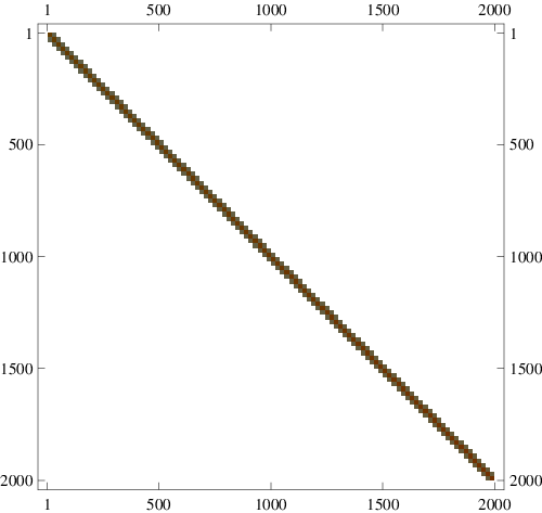
Table 1 shows the ground–state energy of the Rabi Hamiltonian for several values of and for the same set of parameters chosen by Bishop et al[30]. Present results are more accurate than those obtained earlier and will be a useful benchmark for the investigation of the convergence properties of the CMX. We have calculated the matrix analytically in terms arbitrary model parameters so that we do not have to calculate it again each time that we decide to modify those parameters. This strategy makes the calculation quite efficient.
We have calculated the lowest eigenvalues of the matrices by iterative application of the conjugate gradient method (CGM) to the numerical matrix . Notice that our results are fully converged for a matrix, except in the last case considered where just the last digit is not correct.
| 1000 | 1 | 1 | 5 | -100.000626570374178204295743532860688625653449650 |
| 1500 | 1 | 1 | 5 | -100.000626570374178204295743532860688625653449650 |
| 2000 | 1 | 1 | 5 | -100.000626570374178204295743532860688625653449650 |
| ref.[30] | 1 | 1 | 5 | -100.001 |
| 1000 | 1 | 2 | 5 | -50.001262757900797977214814102896046471301336432 |
| 1500 | 1 | 2 | 5 | -50.001262757900797977214814102896046471301336432 |
| 2000 | 1 | 2 | 5 | -50.001262757900797977214814102896046471301336432 |
| ref.[30] | 1 | 2 | 5 | -50.0013 |
| 1000 | 2 | 1 | 5 | -100.002506281526606167493915731790865439561963879 |
| 1500 | 2 | 1 | 5 | -100.002506281526606167493915731790865439561963878 |
| 2000 | 2 | 1 | 5 | -100.002506281526606167493915731790865439561963878 |
| ref.[30] | 2 | 1 | 5 | -100.003 |
3 The cumulant or –expansion
For concreteness, in this section we outline the main ideas behind the so–called –expansion (or cumulant expansion)[1]. The moment–generating function
| (10) |
gives us the moments of the hamiltonian operator , where is a properly chosen trial state. The expectation value of in the state
| (11) |
exhibits several interesting properties: first, , where is the ground–state energy, second, and, third, provided that the overlap between and the ground state is nonzero.
The function is closely related to the cumulant function defined by .[2, 3] The formal Taylor series of about yields the –expansion:
| (12) |
where the cumulant coefficients (or connected moments) can be easily obtained from the recurrence relation
| (13) |
The main advantage of the methods based on the cumulant or connected–moments expansion is that they are size extensive[1, 6].
Any practical application of this method requires a suitable extrapolation of the –expansion (12) to in order to obtain . This is not a simple task and different extrapolation techniques may lead to different results. As we have already mentioned before the first application of the –expansion was based on Padé approximants that provide the simplest and most straightforward strategy[1]. At this point we want to point out a common misconception about the theorem of Horn and Weinstein[1]. Many authors state that the function (12) converges for [5, 12, 13, 28, 17, 20] which is not the case as one can easily verify. For some complex values of the function may vanish and therefore the –expansion converges for where is the singular point of closest to the origin in the complex –plane. This fact has already been discussed by Witte and Shankar[18] and one may easily convince oneself that it is so by means of the exactly solvable two–dimensional model discussed by Knowles[6].
Note that the expansion in terms of exponential functions of
| (14) |
which is the basis of the CMX[5], does not take into account the singular points of and therefore the matching of the –expansion is only valid for . Consequently, it is unlikely that we can successfully extrapolate the expression (14) thus derived to the limit .
Regardless of which extrapolation scheme we may use, it is clear that the application of the theorem proved by Horn and Weinstein requires the calculation of a certain number of connected moments of the Hamiltonian. For problems of great complexity, such as for example many–body or quantum field theory problems, it may be quite difficult (or even impossible) to carry out this task for sufficiently large (or even modest) orders. In such cases one should therefore rely on the extrapolation of the expansion with a few connected moments. It is not easy to prove the accuracy of such extrapolations in the general case, and for this reason it is useful to verify what happens in the case of a simple though non–trivial model, like the Rabi Hamiltonian, where it is possible to obtain large–order moments and sufficiently accurate numerical results. We expect that a careful investigation of the convergence properties of the connected moments expansions for this model will then serve as a guide for others in which one cannot carry out calculations to such large orders.
We first outline the procedures that we follows for the calculation of exact analytical moments of the Hamiltonian. In the first place, we resort to an matrix representation of the Hamiltonian operator, as a function of the parameters of the model. for simplicity we assume that is even, i.e. that we are working in a subspace of the Hilbert space containing at most bosons. If is sufficiently large (for example, ) we can safely calculate the first (say ) moments exactly. The effect of the space truncation does not affect the calculation because of the band form of the matrix shown in Fig. (1) 11 1 The Rabi Hamiltonian allows transitions which involve a change in the number of bosons by one unit and a spin flip. This means that, as long as is chosen large enough, the moments of the Hamiltonian in may be obtained exactly.. In this approximation the moment is simply given by the corresponding diagonal element of . We have also resorted to the coordinate representation and calculated the moments analytically in order to verify the accuracy of the matrix approach just outlined.
In order to calculate the moments we follow Fessatidis et al [14] and choose the trial state to be the ground–state of the noninteracting Hamiltonian (). In this way we can readily calculate the moments of the Rabi Hamiltonian systematically and analytically by straightforward matrix–matrix and matrix–vector multiplications (or in the alternative way indicated above). To this end we resorted to the symbolic operations provided by available computer algebra software like Mathematica and wrote a code that produces the desired moments and connected moments in a reasonably short time. On the other hand, Fessatidis et al [14] only derived the first five moments of the Rabi Hamiltonian, a fact which considerably limited the accuracy of their results as well as the reliability of their conclusions.
Alternatively the moments of the Rabi hamiltonian may be calculated by representing the Hamiltonian operator as
and writing the trial state as
In this way we can obtain moments of sufficiently large order by straightforward differentiation and integration and compare them with those provided by the matrix–vector procedure outlined above.
With the purpose of comparison we show the first five moments calculated in the two ways indicated above:
| (21) |
It is worth noting that our moment is different from the one shown in Eq. (12) of the paper by Fessatidis et al[14]. We have verified that this discrepancy was not merely a misprint so that their results and conclusions may be incorrect. We will come back to this point later on.
Once we have the moments the calculation of the connected moments by means of Eq. (13) is straightforward. The first five ones are
| (22) |

Fig. 2 shows the ratios and for the Rabi Hamiltonian with and . Note that the ratio of the connected moments exhibits an irregular oscillatory behaviour that suggests that we may encounter difficulties in the summation of the –series (in fact, in this case the function proposed by Knowles[6] is not even close to a Stieltjes series).
4 Connected–Moments Expansion
In order to apply the CMX to the Rabi Hamiltonian we resort to the beautifully compact expression for the correlation energy derived by Knowles:[6]
| (23) |
Knowles[6] also discussed the following alternative expression for the correlation energy:
| (24) |
where () and developed by Cioslowski[5]. These two expressions are not equivalent and yield different series in powers of the coupling constant . In this paper we calculate the correlation energy by means of Eq. (23) that appears to be more accurate and suitable for present large–order calculations.
We have been able to obtain a sufficiently large number of moments and connected moments of the Rabi Hamiltonian by means of the procedures described above. The square matrix appearing in Eq. (23) may be badly conditioned and therefore its inverse may contain large numerical errors unless its elements are known with sufficiently large accuracy.
In this paper we have decided to compare the performance of the CMX with that of the Rayleigh–Ritz variational method in the Krylov space (RRK). In the latter approach we choose the nonorthogonal basis set , where is a properly chosen trial state. In this particular implementation of the Rayleigh–Ritz variational method the secular equations become[6, 25, 26, 27]
| (25) |
There are nontrivial solutions to the homogeneous system of linear equations (25) only for the values of that are roots of the secular determinant
| (26) |
It is well known that the Rayleigh–Ritz approximate eigenvalues converge monotonously from above towards the actual eigenvalues of the Hamiltonian operator . In particular, if is not orthogonal to the ground state then approaches the ground–state energy as increases.
We have considered the same set of values of , and used by Fessatidis et al.[14] in their application of the CMX to the Rabi Hamiltonian. For each set of values we have obtained CMX results for that requires up to connected moments. As we have already mentioned, we do not expect to confirm the results of Fessatidis et al[14], even qualitatively, because their approach based on only five moments is affected by an error in .
For concreteness we restrict the discussion to the case and three values of . The conclusions apply to the other cases as well. In order to compare the rate of convergence of the RRK and CMX we calculate where is the approximate ground–state eigenvalue of the Rabi Hamiltonian calculated with moments by means of either method.
Figures 3 and 4 show that the RRK converges faster and more smoothly than the CMX for and , respectively. When the rate of convergence of the RRK is extremely slow. However, although the CMX appears to give better results at some orders, the great oscillations of render this method rather unreliable as shown in Fig. 5. Those figures look quite similar to plots of vs. and are therefore reasonable estimates of the rate of convergence of the moments methods.
5 Conclusions
Some time ago the moments expansions appeared to be a promising tool for the calculation of the ground–state energy of quantum–mechanical problems of physical interest. However, some judicious investigations suggested that the moments expansions are unreliable and that in some cases they can even yield wrong results[6]. In spite of this fact there is still some unclear and inconclusive investigation on the convergence properties of the moments expansions. With the purpose of adding valuable information to that research we have tested the CMX on the Rabi Hamiltonian that has already been treated by means of the moments expansions[14]. We have calculated moments and connected moments of much larger order than those considered before. Our results clearly show that the CMX is unreliable because the successive approaches to the ground–state energy oscillate so strongly that one is never sure of the accuracy of any particular calculation. Lee and Lo[17] arrived at similar conclusions for another model although by numerical calculations of only fifth order.
We have contrasted the CMX with the RRK and showed that the latter converges more smoothly from above towards the exact eigenvalues. It is reasonable to compare these approaches that are based on the same kind of moments of the Hamiltonian operator. Whereas the CMX provides an approximation to the lowest eigenstate–eigenvalue of a given symmetry, the RRK yields all the eigenstates–eigenvalues simultaneously because it is based on the Rayleigh–Ritz variational method. The main advantage of the connected–moments expansions, namely, size consistency[1, 6], is not an issue in the case of simple problems like the one discussed here. In other words: the RRK is preferable to the CMX and its variants in most (if not all) the cases treated so far by means of the connected–moments expansions.
In our opinion most standard approximation methods are more reliable than the moments expansions.
References
References
- [1] Horn D and Weinstein M 1984 Phys. Rev. D 30 1256.
- [2] Cramér H 1946 Mathematical Methods of Statistics (Princeton University Press, Princeton).
- [3] Kubo R 1962 J. Phys. Soc. Jap. 17 1100.
- [4] Stubbins C 1988 Phys. Rev. D 38 1942.
- [5] Cioslowski J 1987 Phys. Rev. Lett. 58 83.
- [6] Knowles P 1987 Chem. Phys. Lett. 134 512.
- [7] Mancini J D, Zhou Y, and Meier P F 1994 Int. J. Quantum Chem. 50 101.
- [8] Cioslowski J 1987 Phys. Rev. A 36 374.
- [9] Cioslowski J 1987 Int. J. Quantum Chem. S 21 563.
- [10] Cioslowski J 1987 Phys. Rev. A 36 3441.
- [11] Cioslowski J 1987 Chem. Phys. Lett. 136 515.
- [12] Massano W J, Bowen S P, and Mancini J D 1989 Phys. Rev. A 39 4301.
- [13] Mancini J D, Prie J D, and Massano W J 1991 Phys. Rev. A 43 1777.
- [14] Fessatidis V, Mancini J D, and Bowen S P 2002 Phys. Lett. A 297 100.
- [15] Fessatidis V, Corvino F A, Mancini J D, Murawski R K, and Mikalopas J 2010 Phys. Lett. A 374 2890.
- [16] Mancini J D, Zhou Y, Meier P F, Massano W J, and D. P J 1994 Phys. Lett. A 185 435.
- [17] Lee K C and Lo C F 1993 Nuovo Cim. D 15 1483.
- [18] Witte N S and Shankar R 1999 Nucl. Phys. B 556 445.
- [19] Mancini J D, Murawski R K, Fessatidis V, and Bowen S P 2005 Phys. Rev. B 72 214405 (6 pp.).
- [20] Fessatidis V, Mancini J D, Murawski R, and Bowen S P 2006 Phys. Lett. A 349 320.
- [21] Fessatidis V, Mancini J D, Bowen S P, and Campuzano M 2008 J. Math. Chem. 44 20.
- [22] Bartashevich I 2008 Int. J. Quantum Chem. 108 272.
- [23] MacDonald J K L 1933 Phys. Rev. 43 830.
- [24] Marmorino M G 2008 Int. J. Quantum Chem. 108 1304.
- [25] Fernández F M, Rayleigh-Ritz variation method and connected-moments polynomial approach, arXiv:0807.1442 [math-ph]
- [26] Fernández F M 2009 Int. J. Quantum Chem. 109 717.
- [27] Amore P and Fernández F M 2009 Phys. Scr. 80 055002 (5pp).
- [28] Šamaj L, Kalinay P, Markoš P, and Traveneč I 1997 J. Phys. A 30 1471.
- [29] Pan F, Guan X, Wang Y, and Draayer J P 2010 J. Phys. B 43 175501 (5 pp).
- [30] Bishop R F, Davidson N J, Quick R M, and van der Walt D M 1999 Phys. Lett. A 254 215.


