IPPP/10/86 ; DCPT/10/172
CERN-PH-TH/2010-234
A slice of AdS5 as the large limit
of Seiberg duality
Steven Abela,b,11 1 s.a.abel@durham.ac.uk and Tony Gherghettac,22 2 tgher@unimelb.edu.au
aInstitute for Particle Physics Phenomenology
Durham University, DH1 3LE, UK
bTheory Division, CERN, CH-1211 Geneva 23, Switzerland
cSchool of Physics, University of Melbourne
Victoria 3010, Australia
A slice of AdS5 is used to provide a 5D gravitational description of 4D strongly-coupled Seiberg dual gauge theories. An (electric) SU gauge theory in the conformal window at large is described by the 5D bulk, while its weakly coupled (magnetic) dual is confined to the IR brane. This framework can be used to construct an MSSM on the IR brane, reminiscent of the original Randall-Sundrum model. In addition, we use our framework to study strongly-coupled scenarios of supersymmetry breaking mediated by gauge forces. This leads to a unified scenario that connects the extra-ordinary gauge mediation limit to the gaugino mediation limit in warped space.
1 Introduction
Seiberg duality [1, 2] is a powerful tool for studying strong dynamics, enabling calculable approaches to otherwise intractable questions, as for example in the discovery of metastable minima in the free magnetic phase of supersymmetric quantum chromodynamics (SQCD) [3] (ISS). Despite such successes, the phenomenological applications of Seiberg duality are somewhat limited, simply by the relatively small number of known examples.
An arguably more flexible tool for thinking about strong coupling is the gauge/gravity correspondence, namely the existence of gravitational duals for strongly-coupled gauge theories [4, 5, 6]. Such duals are known in certain cases to be equivalent to a cascade of Seiberg dualities, the prototypical example being an theory [7, 8], which describes the moduli space of a theory of branes and fractional branes on the warped-deformed conifold (see [9, 10] for reviews). Warped geometries are indeed generally characteristic of compactifications with flux [11]. Metastable ISS-like supersymmetry breaking can be implemented by having various different brane configurations at the end of such throat-like geometries, as in for example [12, 13, 14, 15], and can be successfully mediated as in [16, 17, 18].
It is natural to suppose that these and similar examples can be approximated by the “slice-of-AdS” Randall-Sundrum scenario [19] (RS1). The RS1 formulation provides an ideal framework for discussing the effects of strong coupling without having to use the full complexity of string theory. Indeed the phenomenology is typically dominated by the low energy modes, and the throat itself enters mainly through the Kaluza-Klein (KK) spectrum. Moreover the latter tends to be linear, so that certain phenomena can be rather universal. RS1 can therefore be a useful approximation because precise knowledge of the gravitational dual is often unnecessary, aside from its general scale and warping. One example, again in the context of supersymmetry breaking, is gaugino mediation [20, 21, 22, 23, 24, 25, 26, 27, 28, 29]. There supersymmetry breaking is mediated to scalars localized on the UV brane via bulk gauge modes. However, the resulting suppression of the scalar masses is relatively independent of whether the bulk is flat or warped, and depends only on the separation in the approximately linear KK spectrum.
On the other hand there is an obvious drawback of RS1: it is unclear whether the strongly coupled 4D system that is supposed to correspond to a given configuration actually exists. Because of this it seems interesting to study strongly coupled 4D field theories that have an RS1-like configuration, namely a period of conformal running with a well behaved and calculable perturbative theory in the infra-red. In particular, we would like to begin with simple 4D dynamics that has certain properties (such as supersymmetry breaking), and by taking a strong coupling limit introduce desirable features of extra dimensional physics (such as gaugino mediation).
This paper presents a straightforward method based on Seiberg duality by which such models can be constructed. It works as follows. Suppose one is interested in reproducing an RS1 configuration that has particular weakly coupled theories located on the IR brane, and the UV brane. The holographic principle tells us that the UV theory should exist as elementary degrees of freedom in the 4D theory whereas the IR theory should be composite. Hence the IR theory (including any gauge degrees of freedom) can be identified as the free-magnetic dual of an electric/magnetic pair. Assuming for definiteness that the theory is , SU and vector-like, then there should be fundamental flavours in the IR theory for it to be IR-free. This theory becomes strongly coupled at some scale , above which an electric theory takes over. Many different (indeed an infinity of) electric theories flow to this particular magnetic theory. The canonical one is an asymptotically free SU theory, where . However, consider instead an SU electric theory with flavours, of which have mass , with the rest being massless. If we choose , then this theory is in the conformal window. Above the mass-scale the theory flows to a fixed point and can enjoy an arbitrarily long period of conformal running. At the scale however, we integrate out the heavy flavours, and the theory flows to the same weakly coupled magnetic theory in the IR. Moreover the SU theory approaches strong coupling as . By taking a large limit and adding massive and massless flavours to keep the ratio fixed (the Veneziano limit [30]), one can arrange for the conformal fixed point to be at arbitrarily strong coupling. In this limit, we replace the period of conformal running with a bulk gravitational dual, and arrive at an RS1 configuration, with the global flavour symmetries becoming bulk gauge symmetries, the magnetic theory confined to the IR brane, and any elementary degrees of freedom to which the theory weakly couples, becoming degrees of freedom on the UV brane. In a sense this is simply the shortest possible cascade, in which strong and weak coupling are connected by a single Seiberg duality.
Our bulk is required to be a slice of the gravitational dual of strongly coupled SQCD, whatever that may be. Since the conformal theory has an -symmetry, a good candidate for the geometry is six dimensional, namely with the -symmetry corresponding to translations along the circle, . A solution of this type for general was constructed in Ref. [31] using the effective action of six-dimensional non-critical superstrings. This specific background can be realized with a stack of D3 branes at the tip of the SL cigar, with the flavours of fundamental and antifundamental being provided by space-time filling uncharged D5 branes.
It should be noted that this background is not under good theoretical control. Its curvature is large so the solution will get order one corrections from higher-derivative terms in the effective action. Indeed as argued in Ref. [32] and also in Section 3.3, it is likely that there can never be a weakly curved gravitational dual of SQCD in the conformal window. Nevertheless, it is also likely that the effect of the large curvature will be to change the parameters of the solution in Ref. [31] while leaving its general properties intact [33, 34]. As we have said, for phenomenological purposes these general properties can often be sufficient.
We will present in this paper two applications that illustrate the approach. Following a summary of the Renormalisation Group (RG) properties of SQCD in the next section, and more details of the configuration in Section 3, we will construct an MSSM-on-the-IR-brane type of model, reminiscent of the original RS1 configuration. We begin with the basic MSSM and find the electric theory by identifying with , and then performing an type Seiberg duality. In order to be able to put the electric theory in the conformal window and then take the large limit, the only modification we need to make to the spectrum of the usual MSSM is to include an arbitrary number of heavy Higgs pairs. The left-handed states are all identified as composite states, as are the gauge degrees of freedom of . The right-handed fields on the other hand can be an arbitrary mixture of elementary and composite states (with the latter being identified as the “mesons” of the Seiberg duality). The remaining gauge degrees of freedom are bulk modes.
The second application is to gauge mediation of supersymmetry breaking. There has been recent interest in 4D models that can reproduce the phenomenology associated with gaugino mediation, namely gaugino masses that are much heavier than scalar masses at the mediation scale [20, 21, 22, 23, 24, 25]. While this set-up is simple to configure in extra-dimensional models, the underlying supersymmetry breaking has to be added by hand. The recent interest has therefore been in finding models in which the dynamics of supersymmetry breaking is included [26, 27, 28, 29]. Here we begin with the “simplified gauge mediation” scenario of Murayama and Nomura [35]. We show that taking the large limit of this theory as described above yields a gaugino mediation model in AdS, with metastable supersymmetry breaking on the IR-brane, matter and messenger fields on the UV brane and gauge fields in the bulk, a scenario that has been considered in a number of phenomenological applications [36, 37]. As in conventional gaugino mediation, the scalar mass squareds are generated by (5D) one loop diagrams that are relatively suppressed due to the bulk separation of matter fields and supersymmetry breaking. We find that (in a certain limit) the suppression is of the form where is the bulk contribution to the beta function coefficient, which effectively counts the messenger content of the strongly coupled CFT. This is the strong coupling version of the usual relation that one finds in perturbative extra-ordinary gauge mediation [38]. From this “extra-ordinary gauge mediation limit”, we will show how one can go continuously to the opposite extreme of supersymmetry breaking in AdS by twisted boundary conditions [23], which we refer to as the “gaugino mediation limit”.
2 UV completions of weakly coupled SQCD
We begin by discussing the possible UV completions of SQCD from the Seiberg duality point of view. It is useful to study the flow down from high energies. In the far UV we assume a standard supersymmetric QCD theory which we refer to as the “electric theory”. This is an SU theory with flavours [1, 2]. With no superpotential this theory has a global symmetry. These global symmetries are anomaly free with respect to the gauge symmetry. There is also an anomalous symmetry that will be irrelevant for our discussion. The particle content is shown in Table 1.
| 1 | |||||
| 1 |
Although the features of the RG flow of these theories will be well known to many readers, it is for clarity worth recapping those elements that we need for our discussion11 1 The behaviour of this theory under RG flow has been described in many excellent texts, for example Ref.[10].. The coupling runs according to the exact NSVZ -function [39]
| (1) |
where is the anomalous dimension of the quarks, given at leading order by
| (2) |
Assume that the high energy theory begins in the so-called conformal window,
| (3) |
The theory then runs to a fixed point as can be most easily seen when it is just inside the conformal window, in the limit where . Solving for the vanishing of the beta function gives the anomalous dimension of the quarks to be order and a fixed point at
| (4) |
Decreasing the number of flavours increases the value of the coupling at the fixed point, until in the opposite limit, where , it approaches strong coupling: solving for the vanishing of the beta function there, one finds that
| (5) |
and therefore by Eq.(2) we have . 22 2 Although the anomalous dimension in Eq.(2) is accurate to one loop, the NSVZ beta function in Eq.(1) is exact. Hence even though the precise form of the anomalous dimension is unknown, as long as it can approach arbitrarily close to , a fixed point will be found. This result can also be derived from the fact that at a conformal fixed point the -charges and dimensions of operators are related as dim : this relation and the definition dim give
| (6) |
the same result as that deduced from the vanishing of the NSVZ beta function in Eq.(1)
The theory at the IR fixed point has an equivalent magnetic description. The magnetic dual theory (which we will call ) has a gauged symmetry, where [1, 2]. Its spectrum is given in Table 2. (Throughout we will denote magnetic superfields with small letters and electric superfields with capitals.)
| 1 | |||||
| 1 | |||||
| 1 | 0 |
The two theories satisfy all the usual tests of anomaly and baryon matching if one adds a superpotential
| (7) |
The equation of motion of the elementary meson, then projects the superfluous composite meson out of the moduli space of the magnetic theory. Obviously the magnetic theory is also inside the conformal window, but where the electric description is strongly coupled the magnetic one is weakly coupled, and vice-versa.
Consider the theory with with . In the absence of the coupling the theory would clearly be no different from the original SQCD one; the magnetic dual has and hence a fixed point at
| (8) |
This is not however the fixed point corresponding to that of the electric theory and indeed any non-zero coupling precipitates flow to a new fixed point. The dim argument predicts it to be where
| (9) |
Note that the beta function of the coupling is which indeed vanishes at this point. The anomalous dimensions themselves are
| (10) |
giving
| (11) |
When and both fixed points in the magnetic description are at weak coupling. And in the opposite limit where , both fixed points are at strong coupling with . A numerically evolved example of such flow is shown in Figure 1a: the solid and dashed lines are the flows in the electric and magnetic theories described above. The magnetic theory is indeed seen to flow initially towards the unstable fixed point with , , before ending up at the stable fixed point , . The fixed point values of the couplings indeed obey the above relations.
Now let us consider what happens when we add a relevant deformation to the electric model – i.e. a new term in the superpotential. If this new term breaks the remaining -symmetry the theory will flow, either to a new fixed point, or to an IR-free or asymptotically free theory. The simplest example of such a deformation is a quark mass term in the electric theory:
| (12) |
where are flavour indices. Consider the case where is diagonal of the form
where , and where this value is set at some UV scale, . This term then explicitly breaks both the -symmetry and the global symmetry down to
| (13) |
At low scales one can integrate out quark/antiquark pairs, leaving light flavours. The global symmetry is further broken, but a (different) -symmetry is recovered:
| (14) |
Thus provided that the theory remains in the conformal window and flows to a new fixed point at stronger coupling than the previous one, corresponding to flavours and colours; this is the solid line in Figure 1b. The scale at which one can integrate out the heavy quarks is not simply because the quarks have a dimension which is different from unity. One finds that the mass of the canonically normalised quarks is larger than the energy scale, when the latter drops below a value given by
| (15) |
where is the dimension of . (Note that at weak coupling when this gives the usual perturbative approximation .)
The corresponding deformation in the magnetic theory is a linear meson term that induces a Higgsing; the magnetic superpotential becomes
| (16) |
where the linear term corresponds to the quark mass term and has the same -charge and flavour structure:
This deformation causes of the quarks to acquire VEVs of the form
| (17) |
The gauge symmetry is Higgsed down to where , and quarks remain light. (Note that we assume .) One can arrange for the change in the number of degrees of freedom to be at the same energy scale in both theories by appropriately choosing . This behaviour is shown in Figure 1b.
If one chooses such that then the behaviour is different again (c.f. Figure 1c). At scales below the theory falls out of the conformal window (so to speak) and into the free magnetic range. The gauge coupling of the electric theory hits a Landau pole below and can be matched onto an IR free magnetic description. On the other hand the original magnetic theory flows smoothly (without encountering strong coupling) to the same IR free theory. This is classic quasi-conformal (walking) behaviour (see Ref. [40] for a recent summary).
Note that upon adding the mass deformation the electric and magnetic theories describe the same physics at scales much higher than and also in the far IR well below it. Around however we see that they are very different. Thus it is important to realise that these are two physically distinct types of UV completion of a single IR free theory. The first consists of a Landau pole followed by a relatively strongly coupled conformal UV phase. The second consists of a smooth transition to a weakly coupled conformal theory in the UV. A third possible type of UV completion would of course be the asymptotically free electric Seiberg dual of the IR free theory.
3 A 5D dual description in the strong coupling limit
3.1 The general set-up
One of the three possibilities for the UV completion of the deformed SQCD (with a quark mass term in the electric theory) is a relatively strongly coupled conformal phase in the limit of large . By the AdS/CFT correspondence [4], this phase admits a weakly-coupled 5D gravitational description. Furthermore given that the 4D deformed SQCD is only conformal below a UV scale, with conformal invariance broken by a mass deformation in the IR, the dual description must be a slice of AdS5. A simple way to mimic these features is to introduce a UV brane and an IR brane corresponding to an RS1 scenario [19]. This is a crude approximation to the underlying dynamics of the microscopic theory. Nevertheless as stressed in the Introduction, many of the qualitative features can be understood in this simplified framework, just as AdS/QCD models are thought to encapsulate certain features of QCD. In this subsection we wish first to sketch out the general features that such a description must have, based on known attempts in the literature to construct gravitational duals of strongly coupled SQCD. We then go on to consider the possible 5D configurations that correspond to strongly coupled 4D Seiberg duals.
First the general set-up. We take a slice of AdS and place a UV brane at and an IR brane at a confinement scale loosely associated with (we will discuss this point in more detail below). In order to accommodate the intrinsic U(1)R symmetry, the dual 5D description must actually be AdS. A solution of this type in the conformal window for general was constructed in Ref. [31] from the effective action of six-dimensional non-critical superstrings. Even though this solution is subject to order one corrections from higher-derivative terms in the effective action, it does provide the required background for the strongly-coupled deformed SQCD. In the string frame the effective 5D coupling is [31]
| (18) |
where is the AdS curvature scale, so that in the limit , with the ratio fixed, the theory becomes weakly coupled. The AdS5 curvature scale is of order the string scale and in the conformal window the radius of the circle satisfies .
As a first approximation we can ignore the since its radius remains approximately constant, and consider the 5D spacetime with the fifth dimension compactified on an interval with 3-branes located at (the UV brane) and (the IR brane) where . The AdS5 metric is written using conformal coordinates
| (19) |
where is the 4D Minkowski metric.
The 5D field content is dictated by the AdS/CFT dictionary. In the 4D electric theory (SQCD) at strong coupling, corresponding to , each operator corresponds to a field in the 5D bulk theory. Furthermore, global symmetries of the 4D theory are interpreted as local gauge symmetries in the bulk. Therefore we assume that the 5D theory has an gauge symmetry. Note that the symmetry is associated with the isometry of the . We are interested in a deformation corresponding to chiral symmetry breaking. Therefore we introduce bulk fields and , with corresponding to the vector currents of the quark fields, and a bifundamental field with , corresponding to the operator (in the sense that the UV VEV of determines ). The 5D masses of the bulk fields are determined by the relation, where is the dimension of the corresponding -form operator [5, 6]. For a vector current with this corresponds to massless 5D vector fields. The dimensionality of the bulk field corresponding to the squark bilinear (whose dimension is ) can be deduced from the -charges of in Table 1 to be so that inside the conformal window. Likewise the field corresponding to the quark bilinear has with . The scalar field component of has a 5D mass-squared which approaches at . In the underlying non-critical string theory the vector fields represent 55 strings propagating on the worldvolume of the spacetime filling D5 branes, while represents the open string tachyons on the D5 branes.
The 5D Lagrangian consists of two parts involving a bulk vector supermultiplet containing an vector supermultiplet, and chiral supermultiplet , and an hypermultiplet , containing chiral supermultiplets . It is given by [41, 42, 43, 44]
| (20) |
where with , and is a bulk mass parameter. Note that at the massless level the orbifold breaks the supersymmetry down to supersymmetry. We shall choose the superfield to be even under the orbifold action, and to be odd.
Inserting the -term equations,
| (21) |
into the equations of motion results in a set of well-known bulk solutions for the components of at arbitrary momentum, . The bulk solutions for the zero modes () correspond simply to setting the -terms to zero[41, 42, 44]
| (22) |
where sign forces to be odd and where and are the scalar components of and respectively. Since we are choosing to be odd under the orbifolding then we can just set . Demanding the vanishing of the delta-function contributions to gives the additional constraint
| (23) |
Alternatively this condition can be derived by considering boundaries at and . Generally the solutions then have to be consistent with the vanishing of the boundary terms in the variation of the action:
| (24) | |||||
Setting the component to zero with the solutions of Eq.(22) also gives Eq.(23).
Using the AdS/CFT relation with we find that . The solution in (22) therefore behaves like . These general solutions have to be matched to whatever VEV may acquire due to brane interaction terms. In particular we are interested in deformations of the strongly coupled SQCD by the addition of a quark mass term and a consequent explicit breaking of the chiral symmetry. In the 5D description this corresponds to specifying the UV boundary condition of the bifundamental field , such that
| (25) |
3.2 The gravitational dual descriptions of Seiberg duality
We now connect this AdS picture with the underlying Seiberg duality, in particular identifying the possible configurations of the bulk and brane theories, the location of the various degrees of freedom involved, and the brane superpotentials and .
It is natural to suppose in the RS1 context that the composite degrees of freedom (i.e. the weakly coupled magnetic theory) should be placed on the IR brane. Note that the magnetic gauge fields are forced to appear there because they must be purely emergent degrees of freedom – they can have no bulk presence since that would imply that a global symmetry of the strongly coupled theory has become a gauge theory at low energies, contradicting the theorem of Ref.[45]. We have seen that in order for the underlying strongly coupled theory to have the required mass term, , there must be an additional bulk meson whose UV boundary value, by the bulk/boundary correspondence, acts as a source field for the operator through the interaction
| (26) |
In accord with of the electric Seiberg dual, the value of on the UV brane should be determined by as specified in Eq.(25). Note that as described in Ref.[44], the holographic correspondence in the supersymmetric theory appears as an interaction in the superpotential on the UV boundary. Hence the correspondence is between a source and current superfield so that, in particular, the scalar operator of the CFT couples to the -term of the source superfield.
The fact that is associated with the dynamical degree of freedom in the AdS picture implies that we should base the rest of the structure on the dual-of-the-dual electric theory. To see this, let us briefly return to 4D Seiberg duality and rename the meson in the magnetic theory , so that the superpotential is . (We shall henceforth drop the -couplings unless we are dealing with them specifically, and shall assume them to be of order unity. We shall also for the moment set the dynamical scales of the electric and magnetic theories to be degenerate, .) On performing the dual of this theory one arrives at an alternative (dual-of-the-dual) electric theory with meson and superpotential coupling
| (27) |
The first term of Eq.(27) is of course precisely the required source term of Eq.(26). (The minus sign comes from the matching of dynamical scales in the electric and magnetic theories, as described below in Section 3.3.) One of the checks of Seiberg duality is that this theory flows to the same IR physics as the theory we first started with. Indeed both and have masses of order . Upon integrating them out one finds , leading to the same spectrum and zero superpotential as the original theory. However note that we may also choose to keep all the degrees of freedom and dualise (yet again) to a second magnetic theory. Now the mesons and are to be treated as elementary and a new composite meson is introduced: the superpotential is
| (28) |
Integrating out and leaves us with the magnetic spectrum and superpotential ( where ) as required. It also identifies the two mesons and .
With this in mind, let us now return to the gravitational dual. The 4D discussion above implies two possible gravitational dual configurations in the large limit:
- •
Configuration 1 – a massless meson : In this case, because we have a dynamical , we must add a new elementary meson on the UV brane that has the same quantum numbers as . The superpotential on the UV brane must be
(29) where fixes the UV VEV of through the equation of motion. The superpotential on the IR brane is of the form
(30) Next let us discuss scales. First note that, using , the purely 4D relation in Eq.(15) gives
(31) so that the factor that naturally warps the physical scales in this set-up is . Now, by comparison with Eq.(28), are identified with the compositeness scale, but not directly. Indeed because is a 5D field and have mass dimension . Furthermore canonical normalisation of the fields on the IR brane leads to the physical Yukawa coupling being of order unity, hence the normalised brane fields are , and . Thus once the fields are canonically normalised, the term gives a physical mass that is also naturally warped down by a factor compared to that generated by . (For the most part we will allow and to be free parameters.) The relation of and to the compositeness scale can be determined by the Higgsing in the flavour-block of the magnetic theory corresponding to the heavy quarks of the electric dual: upon canonically normalising the magnetic quarks and using Eqs.(22), (25) and (31), the condition for gives
(32) Thus, since is the physical mass of the heavy quarks in the electric dual, we can identify
as the compositeness scale, and set its value to be . Furthermore the boundary condition in Eq.(23) correctly equates the two canonically normalised mesons and and their masses as
(33) This identifies the heavy mode as being mostly and the orthogonal massless mode as being mostly , provided that . Note that if , then and we recover the standard Seiberg picture in which the massless meson is identified entirely as , and is integrated out. The set-up for this configuration is as shown in Figure 2.
- •
Configuration 2 – no massless meson: In the 4D theory this corresponds to having just the source term in the electric superpotential without the field:
(34) Upon dualizing one finds a magnetic superpotential
(35) Thus both and gain a mass of order and may be integrated out of the low energy theory, leaving no mesons and no superpotential in the magnetic theory. The gravitational dual has a bulk field for every CFT operator so must be there by the bulk/boundary correspondence. Hence the bulk configuration, shown in Figure 3, must be as before but with no additional meson. For the boundary superpotentials in the gravitational dual we have
(36) and
(37)
As the elementary and composite mix, an obvious possible extension is to generalize the picture and have just a single bulk field . However by the bulk/boundary correspondence, the VEV of this field on the UV brane would be identified as the source for an operator in the underlying CFT (i.e. the electric theory). This operator would have to have the same flavour charges as but such an operator is not readily available in the electric Seiberg dual (a possible exception being the case , when the magnetic quarks can be written as electric baryons). Hence although the physics would be similar to that of configuration 1, the direct link to strongly coupled 4D Seiberg duals would be lost.
3.3 Two caveats
In the context of AdS/CFT the flavour symmetries of our strongly coupled 4D theory are weakly gauged, and their RG behaviour (in particular the possibility of Landau poles) is then important. Let us first consider this from a 4D point of view, by returning to the electric theory with with . The SU gauge groups are inside the conformal window, but the (now gauged) flavour groups, , see flavours and colours. However the flavour groups are anomalous and must be cancelled. According to the anomaly matching procedure of ’t Hooft (see below), the flavour anomalies of the electric and magnetic descriptions should both be cancelled by the same spectator sector. In the present case the coefficients of the and anomalies are and respectively. Thus the spectator sector could be an additional fundamentals of and antifundamentals of . The total number of SU flavours is then and colours is . Since one would conclude that a vacuum does not exist for these theories. However one may add additional states with masses around which are charged only under the flavour symmetry. As far as the Seiberg duality is concerned these states are gauge singlets, and clearly their additional contribution to can bring the flavour symmetry within its conformal window as well.
What if one instead has a theory where the flavour symmetries are in the IR-free phase, with effectively ? (We shall encounter an example later.) In that case the flavour symmetries would hit a Landau pole in the UV and another Seiberg duality would be required. From a 4D viewpoint the original SU would in turn become IR-free and lead to a duality cascade involving the flavour symmetry as well (and most likely a duality wall would ensue). This can be averted by instead adding massive gauge states around the scale . These come in vector multiplets; they can be decomposed as an vector and an chiral superfield both in the adjoint. Hence a single massive gauge multiplet contributes to the beta function coefficient and such states can again bring the flavour groups inside the conformal window.
In short therefore, one expects that even from an entirely 4 dimensional point of view, additional massive states can tame the behaviour of the flavour symmetries above the scale should we choose to gauge them. In the 5D AdS picture such states correspond to Kaluza-Klein modes of the bulk gauge fields. The net effect of the coupling to the CFT is that the RG behaviour of the flavour groups becomes logarithmic [46, 47]. A bound results on the contribution that the flavoured degrees of freedom in the CFT make to the beta function in order to avoid Landau poles in the flavour couplings below the UV scale [48]:
| (38) |
When taking the Veneziano limit we necessarily have and hence this translates into an an upper bound on which depends on . For RS1 type scenarios where the flavour symmetries are identified with SM gauge symmetries, and where 1 TeV this bound is very strict, . In other cases, for example when the bulk gauge symmetries are not SM gauge symmetries (with the latter being either emergent symmetries located on the IR brane or having very small values in the IR), or in the “little RS” scenario [49], the bound can be greatly relaxed.
These bounds are generally equivalent to a lower bound on the curvature of any would-be gravitational dual [48]. Indeed the radius of AdS is typically given by where for example for , so that the bound on immediately translates into a bound on . In the sub-critical construction of Ref.[31] which we shall be invoking, we have and then the curvature is quite large anyway, . This is in line with the general expectation of Ref. [32].
This then is the first caveat about the validity of this framework that one must bear in mind. The second is related, and concerns the interpretation of the dynamical scales of the field theory. In particular, the rightmost panel in Figure 1 is the 4D field theoretical situation whose large limit we are supposed to be approximating. But, in the figure, both electric and magnetic theories have their Landau poles around the scale , and look to be strongly coupled there: why then are we entitled to place a weakly coupled theory on the IR brane? The answer can be found in the matching relation for dynamical scales in Seiberg duality which still permits the Landau poles of the electric and magnetic descriptions to be in different places.
To see this, we can return to the 4D theories and “blow up” the running around the scale in order to examine what happens there when we match the two descriptions. Let us treat the dynamical scales of the electric theory () and magnetic theory () more carefully, and temporarily reinstate the coupling which we have been setting to one above. We will need the matching relation for Seiberg duality, which is
| (39) |
expressed in a basis where the quarks of both theories are canonically normalised, and where the magnetic superpotential is written
| (40) |
In Eq.(39), and are the one-loop beta-function coefficients so that
| (41) |
where . For an SQCD theory in the free magnetic phase we have and , so that we get a perturbative overlap of the electric and magnetic descriptions when . In the interval between and both descriptions are in principle valid. The relation is illustrated graphically in Figure 4.
The scale is unknown, nevertheless as shown later in Section 5.1 (see Eq.(75)) one can identify
| (42) |
where is the canonically normalised meson. On dimensional grounds one expects the Kähler potential to have terms of the form
| (43) |
where is some unknown coefficient. The coupling, , is related to this coefficient as
| (44) |
Thus in addition to there are three free (or rather unknown) parameters which we can choose to be , and (with and being determined by Eqs.(39) and (44)).
It is clear from this discussion what must happen near the IR brane when we have the more complicated situation described above, namely a conformal interval terminated by quark mass terms that cause the theory to enter the free magnetic phase below their mass, . In that case the behaviour shown in Figure 5 is perfectly acceptable. Above the coupling does not run. Below the scale the electric coupling quickly becomes non perturbative. But the magnetic theory can be made arbitrarily weakly coupled in this region since is a free parameter, irrespective of how strongly coupled is the electric theory.
3.4 Flow in the Klebanov-Maldacena solution
Klebanov and Maldacena considered the 6d non-critical string action and found an AdS solution in the presence of space filling D5 and anti-D5 branes and with units of RR flux. Despite the fact that these solutions are relatively strongly curved, it is argued that they are a qualitative approximation to the gravitational dual of SQCD. However for our 5D AdS approximation to be valid it is important that the radius of is small and constant. This is indeed the case, and actually the more general solutions of this system can be seen to exhibit some of the features of the flows we see in the gauge theory. The ansatz for the 6d metric in the string frame is
| (45) |
Thus the radius of curvature of the is . The evolutions of the scalars is given by
| (46) |
and where is the dilaton. For constant , the solutions exhibit two typical kinds of behaviour. The choice and is the AdS solution with constant . If we perturb away from this solution it is straightforward to see that the theory will flow to a linear dilaton behaviour in the UV (i.e. as ). The dilaton behaves as with the theory becoming weakly coupled, while for generic starting values of we have (asymptoting as a tanh function), and . This behaviour is clearly seen in Figure 6a where we show and . The flat region is an AdS “slice”, while the left of the plot (the UV) is the linear dilaton region.
It is interesting to look at the solutions when is itself a function of . This is the gravitational equivalent of integrating out heavy quarks below their mass on the gauge side: in this case it would correspond to a recombination of the D5/anti-D5 flavour branes in the bulk. We can mimic this by adjusting by hand at some value of . The resulting behaviour is shown in Figure 6b. A change in flavour perturbs the AdS solution to one with a different curvature and dilaton, with the AdS5 curvature remaining the same. There is an obvious analogy with Figure 1.


3.5 Anomaly matching in RS1
As we have already mentioned the electric and magnetic theories of Tables 1 and 2 are anomalous in the flavour symmetries: for example both the the and anomalies are non-zero. In a purely 4D setting the ‘t Hooft anomaly matching idea asserts that such flavour anomalies should be the same in both theories; the reasoning is that if one were to gauge the flavour symmetries one would have to add a spectator sector charged only under the flavour symmetries in order to cancel these anomalies. However these new sectors would be blind to the SU gauge group and so insensitive to its behaviour. (By analogy, the lepton sector of the Standard Model does not change when QCD confines.) That both electric and magnetic descriptions have the same flavour anomalies is one of the most powerful tests of Seiberg duality in 4D.
Now however the situation has changed: the flavour symmetries really are gauged in the bulk. What, therefore, becomes of anomaly matching – is it even consistent with our picture of AdS as the large limit of Seiberg duality? (See also [37].) In order to address this question let us consider what the spectator sector has to be. Because anomalies do not exist in 5D, the 4D anomalies are associated with contributions localised at the branes [50, 51, 52, 53]. They can be written
| (47) |
where for
| (48) |
Here the gauge fields can be associated with the 4D zero modes up to an overall normalisation since their bulk profiles are flat. The constants receive the following contributions. A left-chiral fundamental fermion localised on the UV (IR) brane contributes (). The contribution from a massless left-chiral bulk fermion is . On an orbifold heavy modes with parities and can give localised anomalies that are equal and opposite on the branes. The contribution from a fundamental fermion with parity is and from a fermion with parity , it is . Finally there is a contribution from a 5D bulk Chern–Simons term which also gives equal and opposite gauge anomaly terms on the branes. In a consistent gauge invariant theory the summed contributions should vanish on both boundaries.
Now let us interpret the bulk and brane fields in terms of Seiberg duality and discuss the roles that they would play in anomaly matching. Fields on the IR brane clearly belong to the magnetic theory – we shall call this contribution . Fields in the bulk have both a composite and an elementary component – they are therefore present in both electric and magnetic theories, and moreover they are singlets of both the magnetic gauge group (because that lives on the IR-brane only) and the electric gauge group. They can therefore be thought of as part of the spectator sector. They contribute the same anomaly at each brane:
where is their total contribution to the 4D anomalies. Finally the Chern-Simons and possibly heavy mode contributions are
As we have said the total contribution must vanish at each boundary. Thus at the IR boundary we have to satisfy
| (49) |
The interpretation in terms of ’t Hooft anomaly matching of the 4D field theories is that a spectator sector added to cancel the anomalies of the magnetic theory would have total anomaly
| (50) |
On the other hand the UV brane has total anomaly
| (51) |
where are the contributions from whatever degrees of freedom are localised on the UV brane. In order to cancel anomaly contributions here we require
| (52) |
But the left hand side of this equation is the total contribution to the flavour anomaly coming from the elementary degrees of freedom that couple to the CFT. This is nothing other than the spectator sector as seen by the underlying electric theory, . Thus the anomaly matching condition (i.e. ) is satisfied: the same spectator sector can serve to cancel anomalies in both the electric and magnetic theories. Note that the essential features of the bulk physics required for this to work are that a) the contributions from the bulk modes are the same at each brane and b) the contributions from the Chern-Simons terms and the heavy modes are equal and opposite.
As an explicit example consider the anomalies when there is a single bulk meson field . In total this contributes to the anomalies (and the negative to the anomaly), with one half appearing at each boundary. The magnetic theory on the IR brane has a contribution of . Hence a would-be spectator sector (including ) that could cancel the anomaly would have to contribute . However the Chern-Simons contribution has to be at the IR-brane. On the UV brane the net anomaly from and the Chern-Simons term is so we have to add additional elementary fields here that contribute to the anomaly. From a 4D perspective the total contribution from the elementary degrees of freedom (i.e. the spectator sector) is then this plus the contribution from , giving the same that we required for the magnetic theory. In this example the elementary sector could be an additional fundamentals of and antifundamentals of .
4 The MSSM in RS1
We now turn to applications of the proposed “large ” limit of Seiberg duality, the first being an explicit realisation of the Randall-Sundrum (RS1) idea, that the particles of the Standard Model arise as composite degrees of freedom on the IR brane of a slice of AdS. Of course in their original proposal Randall and Sundrum were interested in protecting the Higgs mass in non-supersymmetric scenarios. Since we are working in Seiberg duality we will consider the supersymmetric MSSM instead. (This model is morally similar to the super-technicolour models of Ref. [54].)
In Table 3 we show the MSSM theory. This is the theory that we wish to put on the IR brane of a slice of AdS. The advantage of our approach is that we can establish the set-up working mostly in 4D field theory. Following the discussion of the previous sections we will do this by deriving the MSSM as the magnetic dual of an electric theory. Additional states will then be integrated into the latter in order to make the electric phase conformal above some mass scale, and then the “large ” limit will be taken. This last step requires some particle content in the magnetic theory that can be adjusted – this content is an arbitrary number of Higgs pairs, with corresponding to the usual MSSM. The gauge group that we will dualize is .
We assume for concreteness that the Higgs fields, being in vector-like pairs, have a generic range of mass terms, and that the lightest Higgs is the only one that ends up with a VEV (i.e. this is the one that plays the role of the usual MSSM Higgs). One can envisage more complicated cases in which the electroweak breaking is distributed amongst the Higgs pairs. At low scales, the theory runs precisely as the MSSM, with an asymptotically free and a mildly positive beta function for : the group sees an effective flavour number , and the beta function coefficient is given by , so that as usual. At energy scales above the masses of the additional Higgs fields, those states can be “integrated in” to the theory and start to contribute to the running as well. Eventually we have . The running continues unchanged but the beta function of becomes more negative, eventually reaching . Therefore we can expect the theory to reach a Landau pole at some scale , above which an electric description takes over.
In order to get to an electric description we use the Seiberg duality for groups; the electric gauge group is where
| (53) |
The content of the theory is shown in Table 4. In this section we will use the convention that additional Higgs-like states with -parity are denoted either with or , with a suffix to indicate which SM field they resemble charge-wise.
The -parity charges in the electric theory allow the following superpotential (we set all couplings to one and suppress generation indices to avoid clutter):
| (54) |
This theory has a number of features that we should comment on. First the charges of the Higgses, left-handed quarks and left-handed leptons are the opposite of the charges of their magnetic counterparts. This is because the gauge groups other than are playing the role of “flavour” in the Seiberg duality, and as usual those charges must be reversed. Second, note that the right handed fields of the magnetic theory have no counterpart in the electric theory: in fact those fields are composite bound state “mesons” of the electric theory. In addition there are some new states charged under and . These can be identified as the composite “mesons” of the magnetic theory (the term “meson” of course always referring to mesons of the Sp groups):
| (55) |
The trilinear terms in Eq.(54) are simply the superpotential terms associated with that identification (c.f. Eq.(7)). Finally the linear singlet term in Eq.(54) corresponds to the Higgs mass terms of the magnetic theory: the masses are where is the Landau pole scale of the magnetic theory, hence we require that
| (56) |
| singlets |
| singlets | ||||
| singlets |
It is instructive to confirm that the electric theory we have just described does indeed flow to the MSSM (augmented by extra Higgs fields) of Table 3. (As we have presented it, this is in fact nothing other than the test that the dual-of-a-dual gives back the original theory [2].) Upon performing the Seiberg duality of the electric theory we find the spectrum of Table 5. As we have already said, the block of right-handed MSSM fields are bound state “mesons” of the electric theory. The identification is
| (57) |
The third block of states are also composite “mesons” of the magnetic theory:
| (58) |
The superpotential of this theory is
| (59) | |||||
The first set of terms are masses of order so these fields can be integrated out, whereupon we recover the original spectrum of Table 5 and the MSSM superpotential
| (60) |
The first term gives as required the set of masses for the extra Higgs fields (including one for the lightest field that would correspond to the usual “-term” of the MSSM). The trilinear terms are the usual set of Yukawa couplings: in Seiberg duality we have the added bonus that these interactions necessarily arise because the right-handed fields are composite mesons. Naturally there is then the question of how one could explain the hierarchy that we observe in these interactions. This is outside the scope of the present work but is surely an interesting topic for future study.
Having found a candidate electric dual for the MSSM, all that remains is to take the large limit and propose a gravitational dual. In this case we first add into the electric theory the required states to bring it into the conformal window of the Sp group. The free magnetic window is given by
| (61) |
and the conformal window by
| (62) |
Initially (i.e. for the theory of Table 4) the electric theory has and which, as expected, places it within the free magnetic range for any value of .
Now let us add some additional Higgs states but with masses . Below these fields are integrated out and the theory enters the free magnetic phase described above; thus as discussed in section 2 it is the mass which generates the “IR-brane”. We will add an extra pairs of Higgses and so that above we have . In order to bring the electric theory into the conformal window above we can define a parameter such that
| (63) |
so that
| (64) |
We are then free to take the large limit. In this case sending but keeping formally gives a parametrically strongly coupled conformal . Of course none of this changes the magnetic theory which remains the MSSM with some extra Higgses.
Finally we should discuss the running of the SU(3) and groups. The electric theory has a large gauge group . From the point of view of the group this provides a large number of additional flavours. In fact the effective number of flavours contributing to the beta function is
| (65) |
Clearly the group is in principle now highly IR-free in the large limit (and even when ). Usually one would expect the theory to exhibit some sort of cascade behaviour above with hitting a Landau pole. In fact the situation is the one outlined in Section 3.3. In a conformal phase these beta functions are tamed by additional massive modes charged only under (or ) appearing at the scale . From the RS point of view these states appear automatically as the low-lying Kaluza-Klein modes of the bulk gauge and matter fields. As explained, the end result is a logarithmic running and a bound on the value of .
Having made this caveat we can now propose the entire gravitational dual of this theory at large M. The set-up is shown in Figure 7. The group is emergent and so must appear on the IR brane. From the perspective of the strongly coupled theory, the remaining gauge symmetries are flavour symmetries and have to appear in the bulk. From Section 3, it is clear that all the magnetic “quarks” denoted generically by (i.e. ) and every low energy “matter” meson of the Sp groups with R-parity , denoted by (i.e. ), also appear on the IR brane. Moreover as in the field theory on the IR-brane gives the required MSSM superpotential terms.
However there is a further modification required in the gravitational dual because there are bulk fields corresponding to every composite operator of the CFT. Therefore the bulk contains not only the original fields as above denoted generically as ,
but also the bulk fields that did not appear in the field theory, denoted generically by :
As we saw in section 3 the two types of meson are distinguished by the fact that the latter are in configuration 1, with a corresponding set of matter fields (i.e. ) coupling to on the UV brane, whereas the former with no corresponding fields on the UV brane, are in configuration 2. The superpotentials are then given by
| (66) |
where the trilinear couplings automatically contain all the terms consistent with -parity conservation. Recall that as in the field theory all the mesons without a UV counterpart (i.e. the ’s) are massive and can be integrated out of the low energy theory, whereas those with a UV counterpart (i.e. the ’s) leave a light linear combination of and in the low energy theory. Since the wave-function of the can be warped, the remaining light states could be mostly or mostly . Hence the final low energy right-handed fields, can naturally have different degrees of compositeness, while everything charged under must necessarily be entirely composite.
5 General gauge mediation, simplified
5.1 ISS
Our second application is to supersymmetry breaking on the IR brane and its mediation. The “large ” limit of Seiberg duality will clearly yield a version of the metastable supersymmetry breaking mechanism of Intriligator, Seiberg and Shih [3], but in an RS1 configuration similar to those discussed in Refs. [36, 37]. (A string configuration that corresponds to this case was presented in Ref.[55]. This case is morally similar to the metastable superconformal models of Ref.[56].)
The supersymmetry breaking is a feature of the magnetic theory and so one expects it to appear on the IR-brane. Thus proposals for gauge-mediation that were discussed in the context of RS1 should also be applicable to our strongly coupled configuration. One particular application that we would like to revisit is gauge mediation with gaugino masses that are dominant over scalar ones. In the context of extraordinary gauge mediation [38] this corresponds to increasing the “effective number of messengers”, and a region of parameter space that naïvely corresponds to strong coupling. Calculable and explicit models have long been known in the context of extra dimensional models [20, 21, 22, 23, 24, 25, 43, 26]. Interest has been revived recently in 4D models that can achieve the same kind of screening of scalar mass contributions in for example Refs. [26, 27, 28, 29]. Here we shall be using the large limit of the simple perturbative gauge mediation model of Ref.[35] in order to achieve the same effect.
First let us look at the ISS supersymmetry breaking sector and briefly review the model for comparison. Ref.[3] worked in the free-magnetic phase and noted that the classical superpotential in Eq.(16) is of the O’Raifeartaigh type. Supersymmetry breaking occurs because of the so-called rank condition:
| (67) |
can only be satisfied for a rank- submatrix of the where are flavour indices. The height of the potential at the metastable minimum is then given by
| (68) |
where for ease of notation we are again setting the coupling . The supersymmetric minima in the magnetic theory are located by allowing to develop a vev. The and fields acquire masses of and can be integrated out, whereupon one recovers a pure SU Yang-Mills theory with a nonperturbative contribution to the superpotential of the form
| (69) |
This leads to nonperturbatively generated SUSY preserving minima at
| (70) |
where , in accord with the Witten index theorem. The minima can be made to appear far from the origin if is small and , the condition for the magnetic theory to be IR-free. The positions of the minima are bounded by the Landau pole such that they are always in the region of validity of the macroscopic theory.
Now for the holographic version. Following the discussion in Section 2, we work down from the electric theory. In contrast to Ref.[3] we begin in the conformal window but with the global flavour symmetry explicitly broken by relevant mass-terms as
| (71) |
where , and where we choose
| (72) |
We also add to the electric spectrum a superfield that transforms as an adjoint under the symmetry. The superpotential of the electric theory is (we set all Yukawa couplings to one)
| (73) |
where
and where . Initially the model behaves according to the discussion of Section 2; that is at the scale
| (74) |
we can integrate out the heavy quark states. The theory can be dualized to a weakly coupled and IR-free magnetic phase with flavours and a dynamical scale . However the magnetic superpotential is
| (75) |
where
The flavour contractions are self-evident: for example the contraction can involve only those elements of in the upper block. As this is a mass term, the blocks of flavour adjoints may be integrated out supersymmetrically near the Landau pole scale to leave a superpotential
| (76) |
where we now indicate the flavour blocks with indices. Finally, assuming that the mass for and dominates, i.e. that , we may integrate out these fields as well, to find
| (77) |
Since no gauge symmetry has been broken so far, this is an O’Raighfeartaigh theory that has flavours of quarks. We may now take a large limit. In this case, remaining inside the correct ranges of flavours means that and also become large. However there is no such constraint on either or which may both be of order unity. Hence the IR theory can be weakly coupled. Note that this type of SUSY breaking could be inserted directly into the Higgs sector of the MSSM model in the previous subsection.
5.2 General gauge mediation
The metastable SUSY breaking of the previous section lends itself to an RS1 implementation of the “simplified” gauge mediation scenario discussed in Ref. [35]. The result is a holographic version of general gauge mediation [57]. To briefly recap, the 4D picture is as follows. Suppose that the supersymmetry breaking sector (i.e. the sector above) contains no direct connection with the Standard Model gauge groups, , but that there is an additional pair of messenger fields that are charged under . The authors of Ref. [35] argued that one can expect higher order operators to be generated in the underlying electric theory of the form
| (78) |
where is the messenger mass and is the scale of underlying physics, namely the mass scale of new modes in the theory that are exchanged between the messengers and the strongly coupled ISS sector. For convenience we are now (and will henceforth) drop the indices that identify this as the block. In the low energy theory the SUSY breaking and mediation part of the superpotential becomes
| (79) |
As noted in Ref. [35], the first term is precisely the usual spurion interaction of ordinary gauge mediation. However the effective coupling can be very small since generally one expects . The advantage of this suppression is that the -symmetry breaking in the theory is under strict control. Of course the terms in Eq.(79) do explicitly break -symmetry since has -charge 2 (it appears with a linear term in the rest of the superpotential), however it is still approximately conserved because of the smallness of the coupling to the spurion. An equivalent statement (as prescribed by Ref.[58]) is that a new global SUSY preserving minimum is introduced but that it is so far away in field space that it could never disrupt the metastability of the SUSY breaking ISS sector. Indeed it is clear that the linear term can be set to zero if , but this can be much larger than the scale , making it irrelevant to physics in the magnetic theory. The phenomenology of these models is similar to that of conventional gauge mediation (with the main difference being that the NLSP decay length is parametrically longer [59]).
The AdS equivalent of this type of mediation is as shown in Figure 8. We begin with the ISS configuration of the previous section but add the elementary messenger fields on the UV brane. As we have seen an additional meson is required on the UV brane and this will in general mix with the meson through its couplings to the bulk field . We will implicitly assume – in order to justify having bulk gauge bosons – that some of the fields in the non-supersymmetry breaking sector (i.e. the sector above) also couple to the Standard Model gauge groups, but that only the messenger field couples to . In addition we require -symmetry to be broken in the UV theory which is represented by an explicit mass term for the messengers. The brane superpotentials are then by comparison with Eqs.(78) and (79) given by
| (80) |
As we saw this is the theory that remains after all of the confining physics described above has taken place, so that , and represent the fields in the low energy flavour block. Without the term the anomaly-free -symmetry of Table 2 is unbroken. As required by comparison to the ISS model, the term induces an expectation value for on the boundary (equivalent to in the underlying strongly coupled QCD theory by the bulk/boundary correspondence) because of the term in the effective potential. (Note that, as we shall see in a moment, we cannot just set because supersymmetry is broken.) This leaves a residual but anomalous -symmetry. The mass term for the gauginos then breaks the -symmetry entirely on the UV boundary as in Ref.[35], but the IR brane retains it. In this way the gravitational dual description makes it geometrically explicit that the approximate -symmetry of the IR theory is an emergent phenomenon33 3 See Ref.[60] for an alternative example of this phenomenon..
Before presenting precise details, let us describe how we expect the suppressed mediation of Ref.[35] to operate in the gravitational dual description. As we have said, the boundary terms break supersymmetry and enforce a linear combination of the 4D and fields to zero. To see how this happens it is useful to temporarily disregard the effect of warping and consider the 4D theory whose superpotential is simply the sum of and :
| (81) |
One can use the residual flavour symmetry to diagonalise the problem, and it is then easy to see that diagonal components of all the -terms can be set to zero by choosing for . The remaining contributions to the potential are
| (82) |
where to avoid confusion we are using the same symbol for the superfield and its scalar component. Defining a mixing angle
| (83) |
the metastable ISS minimum occurs at
| (84) |
with the effective -terms for and being given by
| (85) |
and with the remaining light meson field being given by
| (86) |
The low energy theory is then
| (87) |
Thus this purely perturbative 4D model is, at energies below , essentially the configuration of [35] and the gauge mediation is standard. In particular note that the field never contributes to supersymmetry breaking.
Now consider the strongly coupled theory modelled by a slice of AdS, depicted in Fig.8. The supersymmetry breaking sector is similar to the model above, but altered in two ways. First, the field is now a bulk field and generally has a profile that warps down the effective . Second, the superpotentials themselves get an overall warp factor, which changes the relative sizes of the supersymmetry breaking contributions to the potential on the two branes. Nevertheless, some coarse aspects of the 4D model above carry over. For example the bulk meson never contributes to the supersymmetry breaking, which is instead shared between the two branes. In the limit of large the supersymmetry breaking will all be on the IR brane. Moreover the interesting 5D dynamics all happens above the scale . Below this scale the theory behaves like the 4D one described above, modulo the warping of parameters. Therefore, if we choose a low messenger mass , then the mediation sector is oblivous to the strong coupling and the low energy phenomenology closely resembles that of Ref.[35]. The gaugino mass comes from the usual one-loop diagram and one finds the usual 4D result:
| (88) |
in the limit of small . The scalar masses, being given by two loop diagrams, are similar in magnitude and, as in the 4D theory above, the phenomenology is similar to that of ordinary gauge mediation.
However new 5D effects will occur if we choose . The scale then defines a resolution scale much smaller than the typical length scale corresponding to the Kaluza-Klein separation. The loop integrals that contribute to supersymmetry breaking are then effected by the localization of supersymmetry breaking on the IR brane. The net result is a suppression of the scalar masses with respect to the gaugino masses which are still given by Eq.(88). Naively one expects the suppression factor to be given by at least an extra loop factor for the scalars while the gauginos are from the AdS viewpoint a tree-level effect. This is nothing other than an AdS form of gaugino mediation very similar to that in Ref.[23]. It is remarkable that via the AdS/CFT correspondence, the simple model of Ref.[35] becomes a straightforward implementation of general gauge mediation [57]! (Note that the scalar mass-squareds in Ref.[23] indeed conform to the general sum-rules derived in Ref.[57].)
After this long heuristic discussion let us now present some precise details. The scales involved are for the IR physics and for the UV physics, with the cuts-off being related as . First the effect of the warping on the supersymmetry breaking: using the bulk solution for the massless modes given in Eq.(22), and taking into account the warp factors in the canonical normalisation of , the low energy potential written in terms of is
| (89) |
and thus our mixing angle is
| (90) |
where the last relation is for the choice of . (The power of reflects the relation between the canonically normalised fields in Eq.(33).) Thus, when and the supersymmetry breaking is pushed to the IR brane. Note that if on the other hand then . The supersymmetry breaking then naively looks to be completely localized on the UV brane, with , but in this case there is no metastability. Instead the non-perturbative terms discussed in Ref.[3] introduce global supersymmetric minima at a distance less than away in field space, and so the Euclidean tunnelling action is of order : the supersymmetry breaking has to be an IR effect.
We can model the supersymmetry breaking gaugino masses with local terms on the branes. The effective operators are given by
| (91) |
where are constants. To determine the value of the coefficients we need the 5D propagators which can be found in Refs.[41, 23, 42, 61]. The bulk gaugino propagator has a denominator of the form
| (92) |
where are Hankel functions of the first kind of order 1, the tilde modification is of the form
| (93) |
where for gauginos, and where the values of for UV and IR branes respectively are
| (94) |
It is straightforward to extract the pole of the propagator by taking the limit, which gives a gaugino mass of
| (95) |
As usual, the effect of the warping is to scale down the masses in the operator on the IR-brane by a factor . Also note that no gaugino mass results if is equal to : in the limit this would correspond to having Dirichlet boundary conditions on both branes.
For simplicity we shall henceforth neglect the small non-zero -term that is induced on the UV brane, setting and focus on the IR-brane contribution. By comparing with Eq.(88) and using the relation , we determine , to find that the gaugino mass is equivalent to an IR-brane localized term of the form
| (96) |
Let us now compute the scalar mass-squared terms to see the suppression44 4 Note that much of this discussion is valid for RS1 models with -terms on the boundary in general.. In order to do this we have to evaluate the one-loop contributions with bulk gauge fields in the loop. The mass-squared terms are given by
| (97) |
where is the quadratic Casimir of the representation and
| (98) |
The gaugino, and gauge boson, propagators (which can be found in Ref.[23]) are evaluated at , since the external squark fields are assumed to be localized on the UV brane. For the gauge bosons we obtain the explicit expression
| (99) |
while the gaugino propagator is given by
| (100) |
where parametrizes the amount of supersymmetry breaking on the IR brane. Note that in the () limit the gaugino wave-function is completely repelled from the IR-brane by the non-zero -term, and one recovers the Green function for twisted boundary conditions, with Neumann (Dirichlet) boundary conditions on the UV (IR)-brane [23], i.e.
| (101) |
The gaugino mass in this case is pure Dirac, and there are no divergences in . We refer to this as the ‘‘gaugino mediation limit’’ 55 5 In order to calculate these well-known results using current correlators, one would have to use the extended formalism of Ref.[62] which includes Dirac masses. The purely Majorana piece gets exponentially suppressed as in [63].. However we are interested in the case when is finite. In order to treat this more general case we use the following simplified expression for the propagator difference:
| (102) |
where
| (103) |
The functions are modified Bessel functions and therefore are real valued. Using (102) we obtain (with ).
| (104) |
The from the Wick rotation of in has been placed on the LHS of (104). In the limit one obtains (using )
| (105) |
This corresponds to the real part of and reproduces the twisted boundary condition result in Ref. [23]. Therefore the scalar mass-squared for finite can be obtained by considering the real part of . Using (104) we find
| (106) |
In the limit we find that as one would expect in normal gauge mediation. The ratio of the scalar masses to the gaugino masses can be parameterised by such that
| (107) |
(Numerically the twisted boundary condition result is equivalent to .) In the limit we have
| (108) |
A part of this ratio comes from the RG running contribution of the Majorana gaugino masses to the scalar mass-squareds. Therefore, as one would expect, the integral (108) is logarithmically divergent when . In order to find the remaining piece we can compare with the complete field theory expression for the contribution to the mass-squareds from each gauge factor (neglecting the running of the gauge couplings) [64]:
| (109) |
The logarithmic piece in the integral for exactly reproduces this RG running. Subtracting this piece, we find that in the large limit the remaining finite contribution to is given by
| (110) |
Numerically, this approximation is accurate to a few percent for say. At first sight the apparent increase of with is a bit puzzling since heuristically one expects the supersymmetry mediation to scalars to tend to a constant, but actually this relation just reflects the “messenger content” in the bulk. Indeed this limit together with the AdS/CFT relation (c.f. Eq.(38)) gives
| (111) |
This is the AdS/CFT equivalent to the perturbative extra-ordinary gauge mediation relation where the contribution to the beta function coefficient is given by the number of messengers , and where we have [38]. Here in the Veneziano limit the CFT contribution to the beta functions coefficients is instead .
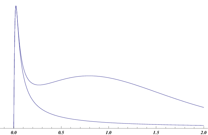
This result was in the limit, which we will refer to as the “extra-ordinary gauge mediation limit”. However one can determine and extract numerically for the general case as we increase . In order to do this we first note that when the integral is no longer divergent. This is to be expected since the gaugino is massive and therefore the logarithmic divergence has a natural IR cut-off about the gaugino mass scale. Indeed as the integrand in Eq.(106) can be approximated by
| (112) |
and this function is peaked at , that is precisely where . The integrand and its approximation are shown in Figure 9. The main feature of the “extra-ordinary gauge mediation limit” is that in this region the gaugino pole is well separated, so that one can define a “messenger scale”, , below which the contribution to the mass-squared integral is well described by the piece in Eq.(109). In order to find for arbitrary therefore, we can divide the integral into two regions, with being identified with the contributions from above the scale where the two curves diverge. We can use the local minimum to define this point, whose location is well approximated by the value of the gaugino mass in the gaugino mediation (large ) limit (i.e. it is at 0.24 TeV for the values chosen above). This procedure ceases to be meaningful for large values of because the pole “melts” into the main contribution. At this point extraordinary gauge mediation behaviour goes over to gaugino mediation behaviour as in Ref.[23]. The numerically evaluated and (in the extra-ordinary GM region) are shown in Fig. 10.
As one final remark, it is worth highlighting the restricted form of general gauge mediation that one derives from this model. It is by now well known that the most general configuration for gauge mediation allows six independent parameters (assuming no CP violating phases in the gaugino sector), three for the gaugino mass terms, and three for the squarks [57]. There are five squark masses in total so this requires two sum rules,
| (113) |
The squark masses derived here and in Ref.[23] (which are realisations of general gauge mediation in AdS) of course have to satisfy these rules. However there are only four free parameters for the models discussed here, not six. Assuming that the gaugino masses are driven by couplings to different -terms or possibly different couplings to the same -term, then they can be free parameters, however the mediation to the sfermions is only a function of the AdS geometry and the suppression is the same for all the Standard Model gauge factors. Therefore the pattern of soft-supersymmetry breaking can be written in terms of the gluino mass and three sfermion mass-squared parameters as follows:
| (114) |
6 Conclusions
We have examined Randall-Sundrum (RS1) like configurations in strongly coupled 4D supersymmetric field theory. By taking a large (Veneziano) limit and combining it with a Seiberg duality, we showed how one can construct a model in which a conformal phase with relevant operators (specifically quark mass terms) flows to a weakly coupled free-magnetic phase. The bulk of these theories is approximated by the construction of Klebanov and Maldacena [31]. The magnetic theory, including its gauge fields, lives entirely on the IR brane as emergent degrees of freedom.
We showed how this construction can be used to derive an RS1 version of the MSSM in which the gauge group is emergent. The and hypercharge gauge bosons are bulk degrees of freedom and correspond to part of the “flavour” symmetries of the Seiberg duality. The right-handed fields are predicted to be entirely elementary, whereas the left-handed fields are predicted to be a mixture of elementary and composite degrees of freedom. (The latter are identified as the mesons of the Seiberg duality.)
We also showed how gaugino mediation can be implemented, by beginning with the Murayama-Nomura model of gauge mediation in Ref. [35] and taking its large limit in the specified manner. The metastable supersymmetry breaking of Ref. [3], being an emergent phenomenon, appears on the IR brane, while the matter fields and messenger fields (being elementary degrees of freedom in the model) are on the UV brane. The Standard Model gauge fields are bulk degrees of freedom and therefore gauginos get masses at leading order, whereas the sfermion mass-squareds, which have to be transmitted through the bulk, are suppressed. The result is an AdS version of extra-dimensional gauge mediation. By varying parameters, the pattern of supersymmetry breaking can be taken from extra-ordinary gauge mediation (i.e. equivalent to a large number of messengers that are integrated out below a typical mass scale) to AdS gaugino mediation similar to that of Ref.[23]. Due to the universal nature of the mediation, the model corresponds to general gauge mediation (with additional Dirac gaugino masses) but with only four free parameters.
Acknowledgements
We thank Mark Goodsell and Jose Santiago for discussions. SAA gratefully acknowledges the Royal Society and the University of Melbourne, and TG the IPPP Durham, for support and hospitality. We also thank Yann Mambrini and Orsay, where part of this work was done. SAA is supported by a Leverhulme Senior Research Fellowship and the European RTN grant “Unification in the LHC era” (PITN-GA-2009-237920). TG is supported by the Australian Research Council.
References
- [1] N. Seiberg, “Electric-magnetic duality in supersymmetric non-abelian gauge theories", Nucl. Phys. B 435(1), 129–146 (1995), [arXiv:hep-th/9411149].
- [2] For a review see K. A. Intriligator and N. Seiberg, “Lectures on supersymmetric gauge theories and electric-magnetic duality,” Nucl. Phys. Proc. Suppl. 45BC, 1 (1996) [arXiv:hep-th/9509066].
- [3] K. A. Intriligator, N. Seiberg and D. Shih, “Dynamical SUSY breaking in meta-stable vacua,” JHEP 0604 (2006) 021 [arXiv:hep-th/0602239].
- [4] J. M. Maldacena, “The large N limit of superconformal field theories and supergravity,” Adv. Theor. Math. Phys. 2, 231 (1998) [Int. J. Theor. Phys. 38, 1113 (1999)] [arXiv:hep-th/9711200].
- [5] S. S. Gubser, I. R. Klebanov and A. M. Polyakov, “Gauge theory correlators from non-critical string theory,” Phys. Lett. B 428 (1998) 105 [arXiv:hep-th/9802109].
- [6] E. Witten, “Anti-de Sitter space and holography,” Adv. Theor. Math. Phys. 2 (1998) 253 [arXiv:hep-th/9802150].
- [7] I. R. Klebanov and A. A. Tseytlin, “Gravity Duals of Supersymmetric SU(N) x SU(N+M) Gauge Theories,” Nucl. Phys. B 578, 123 (2000) [arXiv:hep-th/0002159].
- [8] I. R. Klebanov and M. J. Strassler, “Supergravity and a confining gauge theory: Duality cascades and chiSB-resolution of naked singularities,” JHEP 0008, 052 (2000) [arXiv:hep-th/0007191].
- [9] O. Aharony, S. S. Gubser, J. M. Maldacena, H. Ooguri and Y. Oz, “Large N field theories, string theory and gravity,” Phys. Rept. 323, 183 (2000) [arXiv:hep-th/9905111].
- [10] M. J. Strassler, “The duality cascade,” arXiv:hep-th/0505153.
- [11] S. B. Giddings, S. Kachru and J. Polchinski, “Hierarchies from fluxes in string compactifications,” Phys. Rev. D 66, 106006 (2002) [arXiv:hep-th/0105097].
- [12] S. Kachru, J. Pearson and H. L. Verlinde, “Brane/Flux Annihilation and the String Dual of a Non-Supersymmetric Field Theory,” JHEP 0206, 021 (2002) [arXiv:hep-th/0112197].
- [13] S. Franco, A. Hanany, F. Saad and A. M. Uranga, “Fractional Branes and Dynamical Supersymmetry Breaking,” JHEP 0601, 011 (2006) [arXiv:hep-th/0505040].
- [14] S. Franco and A. M. Uranga, “Dynamical SUSY breaking at meta-stable minima from D-branes at obstructed geometries,” JHEP 0606, 031 (2006) [arXiv:hep-th/0604136].
- [15] R. Argurio, M. Bertolini, S. Franco and S. Kachru, “Gauge/gravity duality and meta-stable dynamical supersymmetry breaking,” JHEP 0701, 083 (2007) [arXiv:hep-th/0610212].
- [16] I. Garcia-Etxebarria, F. Saad and A. M. Uranga, “Local models of gauge mediated supersymmetry breaking in string theory,” JHEP 0608, 069 (2006) [arXiv:hep-th/0605166].
- [17] F. Benini, A. Dymarsky, S. Franco, S. Kachru, D. Simic and H. Verlinde, “Holographic Gauge Mediation,” JHEP 0912, 031 (2009) [arXiv:0903.0619 [hep-th]].
- [18] P. McGuirk, G. Shiu and Y. Sumitomo, “Holographic gauge mediation via strongly coupled messengers,” Phys. Rev. D 81, 026005 (2010) [arXiv:0911.0019 [hep-th]].
- [19] L. Randall and R. Sundrum, “A large mass hierarchy from a small extra dimension,” Phys. Rev. Lett. 83 (1999) 3370 [arXiv:hep-ph/9905221].
- [20] E. A. Mirabelli and M. E. Peskin, “Transmission of supersymmetry breaking from a 4-dimensional boundary,” Phys. Rev. D 58, 065002 (1998) [arXiv:hep-th/9712214].
- [21] D. E. Kaplan, G. D. Kribs and M. Schmaltz, “Supersymmetry breaking through transparent extra dimensions,” Phys. Rev. D 62, 035010 (2000) [arXiv:hep-ph/9911293].
- [22] Z. Chacko, M. A. Luty, A. E. Nelson and E. Ponton, “Gaugino mediated supersymmetry breaking,” JHEP 0001, 003 (2000) [arXiv:hep-ph/9911323].
- [23] T. Gherghetta and A. Pomarol, “A warped supersymmetric standard model,” Nucl. Phys. B 602, 3 (2001) [arXiv:hep-ph/0012378].
- [24] C. Csaki, J. Erlich, C. Grojean and G. D. Kribs, “4D constructions of supersymmetric extra dimensions and gaugino mediation,” Phys. Rev. D 65, 015003 (2002) [arXiv:hep-ph/0106044].
- [25] Z. Chacko, P. J. Fox and H. Murayama, “Localized supersoft supersymmetry breaking,” Nucl. Phys. B 706, 53 (2005) [arXiv:hep-ph/0406142].
- [26] M. McGarrie and R. Russo, “General Gauge Mediation in 5D,” Phys. Rev. D 82 (2010) 035001 [arXiv:1004.3305 [hep-ph]].
- [27] D. Green, A. Katz and Z. Komargodski, “Direct Gaugino Mediation,” arXiv:1008.2215 [hep-th].
- [28] M. McGarrie, “General Gauge Mediation and Deconstruction,” arXiv:1009.0012 [hep-ph].
- [29] M. Sudano, “General Gaugino Mediation,” arXiv:1009.2086 [hep-ph].
- [30] G. Veneziano, “Some Aspects Of A Unified Approach To Gauge, Dual And Gribov Theories,” Nucl. Phys. B 117, 519 (1976).
- [31] I. R. Klebanov and J. M. Maldacena, “Superconformal gauge theories and non-critical superstrings,” Int. J. Mod. Phys. A 19, 5003 (2004) [arXiv:hep-th/0409133].
- [32] F. Bigazzi, R. Casero, A. L. Cotrone, E. Kiritsis and A. Paredes, “Non-critical holography and four-dimensional CFT’s with fundamentals,” JHEP 0510, 012 (2005) [arXiv:hep-th/0505140].
- [33] A. M. Polyakov, “The wall of the cave,” Int. J. Mod. Phys. A 14, 645 (1999) [arXiv:hep-th/9809057].
- [34] A. M. Polyakov, “String theory as a universal language,” Phys. Atom. Nucl. 64, 540 (2001) [Yad. Fiz. 64, 594 (2001)] [Int. J. Mod. Phys. A 16, 4511 (2001)] [arXiv:hep-th/0006132].
- [35] H. Murayama and Y. Nomura, “Gauge mediation simplified,” Phys. Rev. Lett. 98, 151803 (2007) [arXiv:hep-ph/0612186].
- [36] E. Dudas, J. Mourad and F. Nitti, “Metastable Vacua in Brane Worlds,” JHEP 0708, 057 (2007) [arXiv:0706.1269 [hep-th]].
- [37] S. Abel and F. Brummer, “Holographic metastability,” JHEP 1005, 070 (2010) [arXiv:1002.4628 [hep-th]].
- [38] C. Cheung, A. L. Fitzpatrick and D. Shih, “(Extra)Ordinary Gauge Mediation,” JHEP 0807, 054 (2008) [arXiv:0710.3585 [hep-ph]].
- [39] V. A. Novikov, M. A. Shifman, A. I. Vainshtein and V. I. Zakharov, “Exact Gell-Mann-Low Function Of Supersymmetric Yang-Mills Theories From Instanton Calculus,” Nucl. Phys. B 229, 381 (1983).
- [40] D. D. Dietrich, “Quasiconformality and mass,” Phys. Rev. D 82, 065007 (2010) [arXiv:1005.1324 [hep-ph]].
- [41] T. Gherghetta and A. Pomarol, “Bulk fields and supersymmetry in a slice of AdS,” Nucl. Phys. B 586 (2000) 141 [arXiv:hep-ph/0003129].
- [42] D. Marti and A. Pomarol, “Supersymmetric theories with compact extra dimensions in N = 1 superfields,” Phys. Rev. D 64, 105025 (2001) [arXiv:hep-th/0106256].
- [43] T. Gherghetta, “TASI Lectures on a Holographic View of Beyond the Standard Model Physics,” arXiv:1008.2570 [hep-ph].
- [44] G. Cacciapaglia, G. Marandella and J. Terning, “Dimensions of Supersymmetric Operators from AdS/CFT,” JHEP 0906, 027 (2009) [arXiv:0802.2946 [hep-th]].
- [45] S. Weinberg and E. Witten, “Limits On Massless Particles,” Phys. Lett. B 96, 59 (1980).
- [46] A. Pomarol, “Grand Unified Theories without the Desert,” Phys. Rev. Lett. 85, 4004 (2000) [arXiv:hep-ph/0005293].
- [47] N. Arkani-Hamed, M. Porrati and L. Randall, “Holography and phenomenology,” JHEP 0108 (2001) 017 [arXiv:hep-th/0012148].
- [48] M. Reece and L. T. Wang, “Randall-Sundrum and Strings,” JHEP 1007, 040 (2010) [arXiv:1003.5669 [hep-ph]].
- [49] H. Davoudiasl, G. Perez and A. Soni, “The Little Randall-Sundrum Model at the Large Hadron Collider,” Phys. Lett. B 665, 67 (2008) [arXiv:0802.0203 [hep-ph]].
- [50] N. Arkani-Hamed, A. G. Cohen and H. Georgi, “Anomalies on orbifolds,” Phys. Lett. B 516, 395 (2001) [arXiv:hep-th/0103135].
- [51] C. A. Scrucca, M. Serone, L. Silvestrini and F. Zwirner, “Anomalies in orbifold field theories,” Phys. Lett. B 525 (2002) 169 [arXiv:hep-th/0110073].
- [52] R. Barbieri, R. Contino, P. Creminelli, R. Rattazzi and C. A. Scrucca, “Anomalies, Fayet-Iliopoulos terms and the consistency of orbifold field theories,” Phys. Rev. D 66, 024025 (2002) [arXiv:hep-th/0203039].
- [53] S. Groot Nibbelink, H. P. Nilles and M. Olechowski, “Instabilities of bulk fields and anomalies on orbifolds,” Nucl. Phys. B 640 (2002) 171 [arXiv:hep-th/0205012].
- [54] M. Antola, S. Di Chiara, F. Sannino and K. Tuominen, “Minimal Super Technicolor,” arXiv:1001.2040 [hep-ph].
- [55] S. Murthy, “On supersymmetry breaking in string theory from gauge theory in a throat,” JHEP 0708, 013 (2007) [arXiv:hep-th/0703237].
- [56] A. Amariti, L. Girardello, A. Mariotti and M. Siani, “Metastable Vacua in Superconformal SQCD-like Theories,” arXiv:1003.0523 [hep-th].
- [57] P. Meade, N. Seiberg and D. Shih, “General Gauge Mediation,” Prog. Theor. Phys. Suppl. 177 (2009) 143 arXiv:0801.3278 [hep-ph].
- [58] A. E. Nelson and N. Seiberg, “R symmetry breaking versus supersymmetry breaking,” Nucl. Phys. B 416, 46 (1994) [arXiv:hep-ph/9309299].
- [59] S. Abel, M. J. Dolan, J. Jaeckel and V. V. Khoze, “Pure General Gauge Mediation for Early LHC Searches,” arXiv:1009.1164 [hep-ph].
- [60] H. Abe, T. Kobayashi and Y. Omura, “Metastable supersymmetry breaking vacua from conformal dynamics,” Phys. Rev. D 77, 065001 (2008) [arXiv:0712.2519 [hep-ph]].
- [61] R. Contino and A. Pomarol, “Holography for fermions,” JHEP 0411, 058 (2004) [arXiv:hep-th/0406257].
- [62] K. Benakli and M. D. Goodsell, “Dirac Gauginos in General Gauge Mediation,” Nucl. Phys. B 816, 185 (2009) [arXiv:0811.4409 [hep-ph]].
- [63] M. McGarrie and D. C. Thompson, “Warped General Gauge Mediation,” arXiv:1009.4696 [hep-th].
- [64] S. P. Martin, “Generalized messengers of supersymmetry breaking and the sparticle mass spectrum,” Phys. Rev. D 55, 3177 (1997) [arXiv:hep-ph/9608224].