Geometric Approach to Quantum Statistical Mechanics and Application to Casimir Energy and Friction Properties

Let us consider 2 dim Euclidean space $(X,\tau)$ described by the following metric.

	$\displaystyle ds^{2}=dX^{2}+\omega^{2}X^{2}d\tau^{2}=G_{AB}dX^{A}dX^{B}{\quad,}$
	$\displaystyle(X^{A})=(X^{1},X^{2})=(X,\tau){\quad,}\quad(G_{AB})=\mbox{diag}(1,\omega^{2}X^{2}){\quad,}$
	$\displaystyle R_{AB}=0{\quad,}\quad R=G^{AB}R_{AB}=0{\quad,}$		(2)

where $A,B=1,2$. The parameter $\omega$ is the ’spring’ constant with the dimension of mass. We impose the periodicity (period: $\beta$) in the direction of the extra dimension $\tau$.

$\displaystyle\tau\rightarrow\tau+\beta{\quad.}$

(3)

This is a way to introduce the temperature ($1/\beta$) in the system. Here we take a path $\{x(\tau),\ 0\leq\tau\leq\beta\}$ in the 2D bulk space (X,$\tau$) and the induced metric on the line is given by

	$\displaystyle X=x(\tau){\quad,}\quad dX={\dot{x}}d\tau{\quad,}\quad{\dot{x}}\equiv\frac{dx}{d\tau}{\quad,}\quad 0\leq\tau\leq\beta{\quad,}$
	$\displaystyle ds^{2}=({\dot{x}}^{2}+\omega^{2}x^{2})d\tau^{2}{\quad.}$		(4)

See Fig.1.

Then the length L of the path $x(\tau)$ is given by

$\displaystyle L=\int ds=\int_{0}^{\beta}\sqrt{{\dot{x}}^{2}+\omega^{2}x^{2}}d\tau{\quad.}$

(5)

We take the half of the length (${\frac{1}{2}}L$) as the system Hamiltonian (minimal length principle). Then the free energy $F$ of the system is given by

$\displaystyle\e^{-\beta F}=\int_{-\infty}^{\infty}d\rho\int_{\begin{array}[]{c}x(0)=\rho\\ x(\beta)=\rho\end{array}}\prod_{\tau}{\cal D}x(\tau)\exp\left[-{\frac{1}{2}}\int_{0}^{\beta}\sqrt{{\dot{x}}^{2}+\omega^{2}x^{2}}d\tau\right]{\quad,}$

where the path-integral is done for all possible paths with the indicated boundary condition (b.c.). This quantum statistical system can be regarded as the square-root type (’Dirac’ type) of the ordinary harmonic oscillator. ¹¹ 1 The situation reminds us of the relation between Nambu-Goto action and Polyakov action in the string theory[17]. The introduction of an auxiliary variable helps to ’normalize’ the square-root action (2.1). In this case, the geometric role of the auxiliary variable remains obscure.

Now we consider another type of 2 dim Euclidean space $(X,\tau)$ described by the following line element.

$\displaystyle ds^{2}=\frac{1}{d\tau^{2}}(dX^{2})^{2}+\omega^{4}X^{4}d\tau^{2}+2\omega^{2}X^{2}dX^{2}=\frac{1}{d\tau^{2}}(dX^{2}+\omega^{2}X^{2}d\tau^{2})^{2}{\quad,}$

(9)

where we put the following condition on the infinitesimal quantities, $d\tau^{2}$ and $dX^{2}$, in order to keep all terms of (9) in the same order.

	$\displaystyle\mbox{[Line Element Regularity Condition]}\ :\quad\quad\quad\quad\quad\quad\quad$
	$\displaystyle d\tau^{2}\sim O(\epsilon^{2}){\quad,}\quad dX^{2}\sim O(\epsilon^{2}){\quad,}\quad\frac{1}{d\tau^{2}}dX^{2}\sim O(1){\quad,}$		(10)

where $\epsilon$ is an arbitrary infinitesimal parameter with the dimension of length. ²² 2 The condition (10) restricts the trajectory configuration (12) only to smooth-lines in the 2D bulk space, and excludes singular-lines which have some singular points (the derivative along $\tau$ can not be defined) between $0\leq\tau\leq\beta$. See Fig.2 for singular and regular lines.

Note that we do not have 2D metric in this case. (We cannot define the bulk metric $G_{AB}(X)$.) We impose the periodicity (period: $\beta$).

$\displaystyle\tau\rightarrow\tau+\beta{\quad.}$

(11)

Here we take a path $\{x(\tau),\ 0\leq\tau\leq\beta\}$, and the induced metric on the line is given by

	$\displaystyle X=x(\tau){\quad,}\quad dX={\dot{x}}d\tau{\quad,}\quad{\dot{x}}\equiv\frac{dx}{d\tau}{\quad,}\quad 0\leq\tau\leq\beta{\quad,}$
	$\displaystyle ds^{2}=({\dot{x}}^{2}+\omega^{2}x^{2})^{2}d\tau^{2}{\quad.}$		(12)

In the bulk we do not have the metric, but on the path, we do have this induced metric. Then the length L of the path $x(\tau)$ is given by

$\displaystyle L[x(\tau)]=\int ds=\int_{0}^{\beta}({\dot{x}}^{2}+\omega^{2}x^{2})d\tau{\quad.}$

(13)

Hence, taking ${\frac{1}{2}}L$ as the Hamiltonian (minimal length principle), the free energy $F$ of the system is given by

$\displaystyle\e^{-\beta F}=\int_{-\infty}^{\infty}d\rho\int_{\begin{array}[]{c}x(0)=\rho\\ x(\beta)=\rho\end{array}}\prod_{\tau}{\cal D}x(\tau)\exp\left[-{\frac{1}{2}}\int_{0}^{\beta}({\dot{x}}^{2}+\omega^{2}x^{2})d\tau\right]{\quad,}$

where the path-integral is done for all possible paths with the indicated b.c.. This is exactly the free energy of the harmonic oscillator. See Feynman’s textbook[18]. ³³ 3 $F=\frac{\omega}{2}+\frac{1}{\beta}\ln(1-\e^{-\beta\omega}),E=<\frac{L}{2}>=\frac{\omega}{2}\coth(\frac{\omega\beta}{2})=\frac{\omega}{2}+\frac{\omega}{\e^{\omega\beta}-1},S=\frac{1}{T}(E-F)=k\{\frac{\beta\omega}{2}\coth\frac{\beta\omega}{2}-\frac{\beta\omega}{2}-\ln(1-\e^{-\beta\omega})\}$

Note that the condition (10) is necessary for the elastic view to the path.

We start with the following metric in 2 dim Euclidean space $(X,\tau)$.

	$\displaystyle ds^{2}=dX^{2}+2V(X)d\tau^{2}=G_{AB}dX^{A}dX^{B}{\quad,}$
	$\displaystyle(X^{A})=(X^{1},X^{2})=(X,\tau){\quad,}\quad(G_{AB})=\mbox{diag}(1,2V(X)){\quad,}$
	$\displaystyle(R_{AB})=\left(\begin{array}[]{cc}\frac{V^{\prime\prime}}{2V}-\frac{1}{4}\left(\frac{V^{\prime}}{V}\right)^{2},&0\\ 0{\quad,}&V^{\prime\prime}-{\frac{1}{2}}\frac{(V^{\prime})^{2}}{V}\end{array}\right){\quad,}\quad R=G^{AB}R_{AB}=\frac{V^{\prime\prime}}{V}-{\frac{1}{2}}\left(\frac{V^{\prime}}{V}\right)^{2}{\quad,}$
	$\displaystyle V^{\prime}\equiv\frac{dV(X)}{dX}{\quad,}\quad V^{\prime\prime}\equiv\frac{d^{2}V(X)}{dX^{2}}{\quad,}$		(21)

where $A,B=1,2$. Note that V(X) does not depend on $\tau$. We impose the periodicity (period: $\beta$) in the direction of the extra dimension $\tau$ (3). On a path $\{x(\tau),\ 0\leq\tau\leq\beta\}$, the induced metric is given by

$\displaystyle ds^{2}=({\dot{x}}^{2}+2V(x))d\tau^{2}{\quad,}\quad 0\leq\tau\leq\beta{\quad.}$

(22)

Hence the length L of the path $x(\tau)$ is given by

$\displaystyle L=\int ds=\int_{0}^{\beta}\sqrt{{\dot{x}}^{2}+2V(x)}d\tau{\quad.}$

(23)

Taking the half of the length (${\frac{1}{2}}L$) as the Hamiltonian, we get the free energy $F$ as

$\displaystyle\e^{-\beta F}=\int_{-\infty}^{\infty}d\rho\int_{\begin{array}[]{c}x(0)=\rho\\ x(\beta)=\rho\end{array}}\prod_{\tau}{\cal D}x(\tau)\exp\left[-{\frac{1}{2}}\int_{0}^{\beta}\sqrt{{\dot{x}}^{2}+2V(x)}d\tau\right]{\quad.}$

We start with the following line element.

$\displaystyle ds^{2}=\frac{1}{d\tau^{2}}(dX^{2})^{2}+4V(X)^{2}d\tau^{2}+4V(X)dX^{2}=\frac{1}{d\tau^{2}}\left(dX^{2}+2V(X)d\tau^{2}\right)^{2}{\quad,}$

(27)

where we put the condition (10) on the infinitesimal quantities, $d\tau^{2}$ and $dX^{2}$, in order to keep all terms in the same order. The 2D bulk space do not have 2D metric. We impose the periodicity (period: $\beta$) (11). On a path $\{x(\tau),\ 0\leq\tau\leq\beta\}$, we have the induced metric:

$\displaystyle ds^{2}=({\dot{x}}^{2}+2V(x))^{2}d\tau^{2}{\quad.}$

(28)

The length L is given by

$\displaystyle L[x(\tau)]=\int ds=\int_{0}^{\beta}({\dot{x}}^{2}+2V(x))d\tau{\quad.}$

(29)

Taking ${\frac{1}{2}}L$ as the Hamiltonian, the free energy $F$ is given by

$\displaystyle\e^{-\beta F}=\int_{-\infty}^{\infty}d\rho\int_{\begin{array}[]{c}x(0)=\rho\\ x(\beta)=\rho\end{array}}\prod_{\tau}{\cal D}x(\tau)\exp\left[-{\frac{1}{2}}\int_{0}^{\beta}({\dot{x}}^{2}+2V(x))d\tau\right]{\quad,}$

where the path-integral is done for all possible paths with the indicated b.c.. This is exactly the free energy of the quantum statistical system of one variable $x$ in the general potential V($x$).

Let us consider N+1 dim Euclidean space $(X^{i},\tau),i=1,2,\cdots,N$ described by the following metric.

	$\displaystyle ds^{2}=\sum_{i=1}^{N}(dX^{i})^{2}+\omega^{2}d\tau^{2}\sum_{i=1}^{N}(X^{i})^{2}=\sum_{i=1}^{N}(dX^{i})^{2}+\omega^{2}r^{2}d\tau^{2}=G_{AB}dX^{A}dX^{B}{\quad,}$
	$\displaystyle A,B=1,2,\cdots,N,N+1;\quad X^{N+1}\equiv\tau{\quad,}\quad$
	$\displaystyle(G_{AB})=\mbox{diag}(1,1,\cdots,1,\omega^{2}r^{2}){\quad,}\quad r^{2}\equiv\sum_{i=1}^{N}(X^{i})^{2}{\quad.}$		(33)

(Subsec.2.1 is the $N=1$ case. ) The Ricci tensor and the scalar curvature are, for N=2, given by ⁴⁴ 4 All curvature calculation in this work is checked by the algebraic calculation soft ”Maxima”[19].

	$\displaystyle ds^{2}=dx^{2}+dy^{2}+\omega^{2}(x^{2}+y^{2})d\tau^{2}{\quad,}$
	$\displaystyle\left(R_{AB}\right)=\frac{1}{(r^{2})^{2}}\left(\begin{array}[]{ccc}y^{2}&-xy&0\\ -yx&x^{2}&0\\ 0&0&\omega^{2}(r^{2})^{2}\end{array}\right){\quad,}\quad R=\frac{2}{r^{2}}>0{\quad,}\quad r^{2}=x^{2}+y^{2}{\quad,}$
	$\displaystyle\sqrt{G}=\omega\sqrt{x^{2}+y^{2}}{\quad,}\quad\sqrt{G}R=\frac{2\omega}{\sqrt{x^{2}+y^{2}}}$		(38)

where $(X^{1},X^{2},X^{3})=(x,y,\tau)$ is taken.

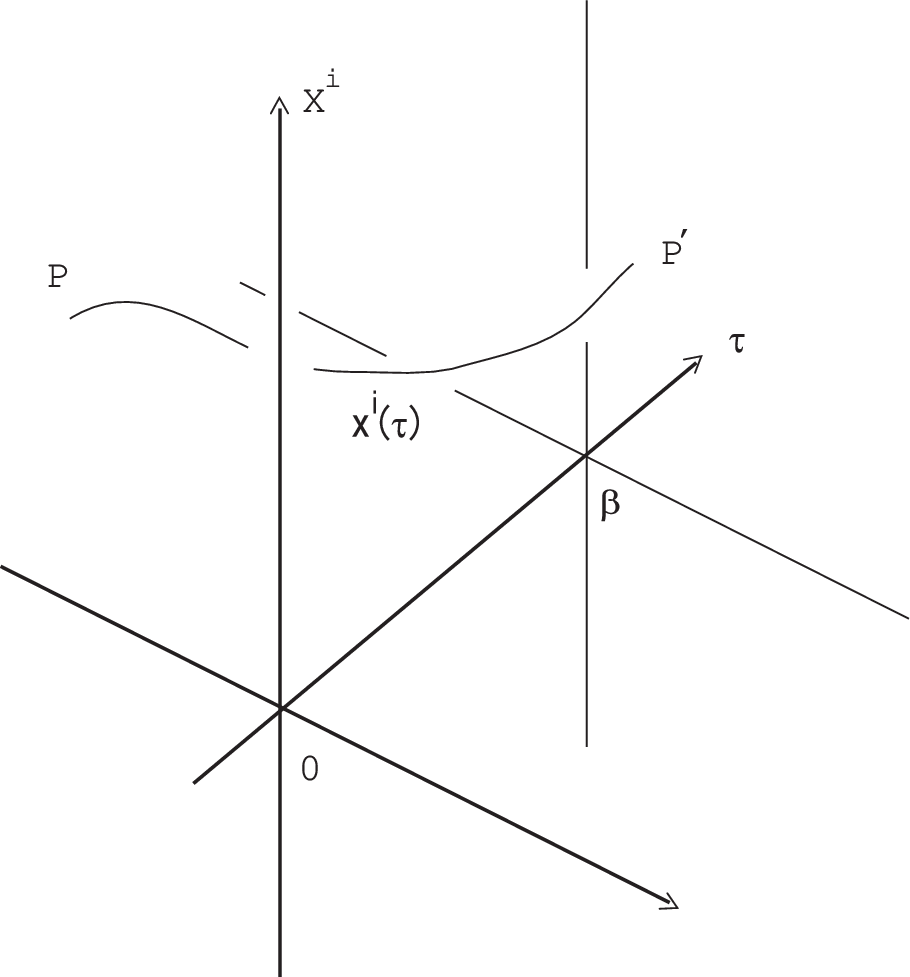
We impose the periodicity (3)(period: $\beta$), and take a path $\{X^{i}=x^{i}(\tau)|\ 0\leq\tau\leq\beta,\ i=1,2,\cdots,N\}$(See Fig.3). The induced metric on the line is given by

	$\displaystyle X^{i}=x^{i}(\tau){\quad,}\quad dX^{i}={\dot{x}}^{i}d\tau{\quad,}\quad{\dot{x}}^{i}\equiv\frac{dx^{i}}{d\tau}{\quad,}\quad 0\leq\tau\leq\beta{\quad,}$
	$\displaystyle i=1,2,\cdots,N{\quad,}\quad ds^{2}=\sum_{i=1}^{N}(({{\dot{x}}}^{i})^{2}+\omega^{2}(x^{i})^{2})d\tau^{2}{\quad.}$		(39)

Then the length L of the path $\{x^{i}(\tau)\}$ is given by

$\displaystyle L=\int ds=\int_{0}^{\beta}\sqrt{\sum_{i=1}^{N}(({\dot{x}}^{i})^{2}+\omega^{2}{(x^{i})}^{2})}~d\tau{\quad.}$

(40)

We take the half of the length (${\frac{1}{2}}L$) as the system Hamiltonian(minimal length principle). Then the free energy $F$ of the system is given by

$\displaystyle\e^{-\beta F}=(\prod_{i}\int_{-\infty}^{\infty}d\rho_{i})\int_{\begin{array}[]{c}x^{i}(0)=\rho_{i}\\ x^{i}(\beta)=\rho_{i}\end{array}}\prod_{\tau,i}{\cal D}x^{i}(\tau)\exp\left[-{\frac{1}{2}}\int_{0}^{\beta}\sqrt{\sum_{i=1}^{N}(({\dot{x}}^{i})^{2}+\omega^{2}{x^{i}}^{2})}d\tau\right]{\quad,}$

where the path-integral is done for all possible paths $\{x^{i}(\tau);i=1,2,\cdots N\}$ with the indicated b.c.. We can regard this as the free energy for a variation (’Dirac’ type) of the N harmonic oscillators’s. (See next subsection for the ordinary type of the N harmonic oscillators.)

Instead of the length $L$, we can take another geometric quantity. Let us consider the following N dim hypersurface in N+1 dim space (a closed-string configuration). See Fig.4 for the N=2 case.

$\displaystyle\sum_{i=1}^{N}(X^{i})^{2}=r^{2}(\tau){\quad,}\quad\sum_{i=1}^{N}X^{i}dX^{i}=r\dot{r}d\tau{\quad,}\quad 0\leq\tau\leq\beta{\quad.}$

(44)

The form of $r(\tau)$ describes a path (N dimensional hypersurface in the bulk) which is isotropic in the ’brane’ at $\tau$ (the N dim space ’perpendicularly’ standing at $\tau$ of the extra axis, not the hypersurface ). The induced metric on the N dim hypersurface is given by

	$\displaystyle ds^{2}=\sum_{i,j}(\delta_{ij}+\frac{\omega^{2}}{\dot{r}^{2}}x^{i}x^{j})dx^{i}dx^{j}\equiv\sum_{i,j}g_{ij}dx^{i}dx^{j}{\quad,}$
	$\displaystyle g_{ij}=\delta_{ij}+\frac{\omega^{2}}{\dot{r}^{2}}x^{i}x^{j}{\quad,}\quad r^{2}=\sum_{i=1}^{N}(x^{i})^{2}{\quad,}\quad\det(g_{ij})=1+\frac{\omega^{2}r^{2}}{\dot{r}^{2}}{\quad.}$		(45)

This is the metric of a O(N) nonlinear system and is the one dimensional nonlinear sigma model as the field theory. ( The standard model (2 dim nonlinear sigma model) has often been used so far in order to show the renormalization group behavior of various systems. The background (effective action) formulation of the string theory heavily relies on the model.) Then the area of the N dim hypersurface is given by

$\displaystyle A_{N}=\int\sqrt{\det g_{ij}}~d^{N}x=\frac{N\pi^{N/2}}{\Gamma(\frac{N}{2}+1)}\int\sqrt{\dot{r}^{2}+\omega^{2}r^{2}}r^{N-1}d\tau{\quad.}$

(46)

When we take ${\frac{1}{2}}A_{N}$ as the Hamiltonian (minimal area principle), the free energy $F$ is given by

$\displaystyle\e^{-\beta F}=\int_{0}^{\infty}d\rho\int_{\begin{array}[]{c}r(0)=\rho\\ r(\beta)=\rho\end{array}}\prod_{\tau,i}{\cal D}x^{i}(\tau)\exp\left[-{\frac{1}{2}}\frac{N\pi^{N/2}}{\Gamma(\frac{N}{2}+1)}\int\sqrt{\dot{r}^{2}+\omega^{2}r^{2}}r^{N-1}d\tau\right]{\quad.}$

We should compare this result ($N=4$) with the proposed 5D Casimir energy for the flat geometry (90). The component $\sqrt{\dot{r}^{2}+\omega^{2}r^{2}}$ in the integrand of (4.1) is replaced by $\sqrt{\dot{r}^{2}+1}$ in (90).

We recognize, if we start with

$\displaystyle ds^{2}=\sum_{i=1}^{N}(dX^{i})^{2}+d\tau^{2}\quad(\mbox{N+1 dim Euclidean flat}){\quad,}$

(50)

instead of (33), the integration measure becomes exactly the same as (90).

Now we consider another type of N+1 dim Euclidean space $(X^{i},\tau);\ i=1,2,\cdots N$ described by the following line element.

	$\displaystyle ds^{2}=d\tau^{-2}\{\sum_{i=1}^{N}(dX^{i})^{2}\}^{2}+\omega^{4}\{\sum_{i=1}^{N}(X^{i})^{2}\}^{2}d\tau^{2}+2\omega^{2}\{\sum_{i=1}^{N}(X^{i})^{2}\}\{\sum_{j=1}^{N}(dX^{j})^{2}\}$
	$\displaystyle=\frac{1}{d\tau^{2}}\{\sum_{i=1}^{N}(dX^{i})^{2}+\omega^{2}r^{2}d\tau^{2}\}^{2}{\quad,}\quad r^{2}=\sum_{i=1}^{N}(X^{i})^{2}{\quad,}$		(51)

with the condition:

	$\displaystyle\mbox{[Line Element Regularity Condition]}\ :\quad\quad\quad\quad\quad\quad$
	$\displaystyle d\tau^{2}\sim O(\epsilon^{2}){\quad,}\quad(dX^{i})^{2}\sim O(\epsilon^{2}){\quad,}\quad\frac{1}{d\tau^{2}}\{\sum_{i=1}^{N}(dX^{i})^{2}\}\sim O(1)\ ,\$		(52)

in order to keep all terms of (51) in the order of $\epsilon^{2}$. ⁵⁵ 5 As in (10), this condition restricts the trajectory configuration (53) only to smooth hyper-surfaces in the (N+1)-dim space. Again we note that, in the above case, we do not have N+1 dim (bulk) metric. We impose the periodicity (3): (period: $\beta$).

Here we take a path of Fig.3: $\{x^{i}(\tau)|\ 0\leq\tau\leq\beta,i=1,2,\cdots,N\}$ and the induced metric on the path is given by

	$\displaystyle X^{i}=x^{i}(\tau){\quad,}\quad dX^{i}={\dot{x}}^{i}d\tau{\quad,}\quad{\dot{x}}^{i}\equiv\frac{dx^{i}}{d\tau}{\quad,}\quad 0\leq\tau\leq\beta{\quad,}$
	$\displaystyle ds^{2}=[\sum_{i=1}^{N}(({\dot{x}}^{i})^{2}+\omega^{2}(x^{i})^{2})]^{2}d\tau^{2}{\quad.}$		(53)

Then the length L of the path $\{x^{i}(\tau)\}$ is given by

$\displaystyle L[x^{i}(\tau)]=\int ds=\int_{0}^{\beta}\sum_{i=1}^{N}(({\dot{x}}^{i})^{2}+\omega^{2}(x^{i})^{2})d\tau{\quad.}$

(54)

Hence, taking ${\frac{1}{2}}L$ as the Hamiltonian (minimal length principle ), the free energy $F$ of the system is given by

$\displaystyle\e^{-\beta F}=\left(\prod_{i}\int_{-\infty}^{\infty}d\rho_{i}\right)\int_{\begin{array}[]{c}x^{i}(0)=\rho_{i}\\ x^{i}(\beta)=\rho_{i}\end{array}}\prod_{i,\tau}{\cal D}x^{i}(\tau)\exp\left[-{\frac{1}{2}}\int_{0}^{\beta}\sum_{i=1}^{N}(({\dot{x}}^{i})^{2}+\omega^{2}(x^{i})^{2})d\tau\right],$

where the path-integral is done for all possible paths with the indicated b.c.. This is exactly the free energy of N harmonic oscillators.

We note again the condition (52) is necessary for the elastic view to the hyper-surfaces.

Instead of (51), we can start from a slightly modified metric.

	$\displaystyle ds^{2}=\omega^{4}\{\sum_{i=1}^{N}(X^{i})^{2}\}^{2}d\tau^{2}+2\omega^{2}\kappa\{\sum_{i=1}^{N}(X^{i})^{2}\}\{\sum_{j=1}^{N}(dX^{j})^{2}\}$
	$\displaystyle=\omega^{2}r^{2}\left(\omega^{2}r^{2}d\tau^{2}+2\kappa\sum_{j=1}^{N}(dX^{j})^{2}\right){\quad,}\quad r^{2}=\sum_{i=1}^{N}(X^{i})^{2}{\quad.}$		(58)

We drop the first term of (51), and add a free (real) parameter $\kappa$ in the third one. We stress that, in this case, we need not the condition of (52). The line element is the ordinary type and we have the bulk metric $G_{AB}$ in this case. The Ricci tensor and the scalar curvature, for $N=2$, are given by

	$\displaystyle ds^{2}=\omega^{4}(x^{2}+y^{2})^{2}d\tau^{2}+2\omega^{2}\kappa(x^{2}+y^{2})(dx^{2}+dy^{2}){\quad,}$
	$\displaystyle\left(R_{AB}\right)=\frac{1}{(r^{2})^{2}}\left(\begin{array}[]{ccc}4y^{2}&-4xy&0\\ -4yx&4x^{2}&0\\ 0&0&\frac{2\omega^{2}}{\kappa}(r^{2})^{2}\end{array}\right){\quad,}\quad R=\frac{4}{\kappa\omega^{2}(r^{2})^{2}}{\quad,}\quad r^{2}=x^{2}+y^{2}{\quad,}$
	$\displaystyle\sqrt{G}=2\omega^{4}|\kappa|r^{4}{\quad,}\quad\sqrt{G}R=8\omega^{2}\cdot\mbox{sign}(\kappa){\quad,}$		(63)

where $(X^{1},X^{2},X^{3})=(x,y,\tau)$ and sign$(\kappa)$ is the sign of $\kappa$. ⁶⁶ 6 $R>0\quad\mbox{for}\quad\kappa>0{\quad,}\quad R<0\quad\mbox{for}\quad\kappa<0$. We consider the N dim hypersurface (44), or Fig.4, and the induced metric on it is given by

$\displaystyle ds^{2}=\sum_{i,j=1}^{N}2\omega^{2}r^{2}(\kappa\delta_{ij}+{\frac{1}{2}}\frac{\omega^{2}}{\dot{r}^{2}}x^{i}x^{j})dx^{i}dx^{j}\equiv\sum_{i,j}g_{ij}dx^{i}dx^{j}{\quad.}$

(64)

Then the area of this hypersurface is given by

$\displaystyle A_{N}=\int\sqrt{\det g_{ij}}~d^{N}x=\frac{(2\pi\omega^{2}|\kappa|)^{N/2}}{\Gamma(\frac{N}{2}+1)}\int_{0}^{\beta}r^{N}\sqrt{\dot{r}^{2}+\frac{r^{2}\omega^{2}}{2|\kappa|}}~r^{N-1}d\tau{\quad.}$

(65)

Taking ${\frac{1}{2}}A_{N}$ as the Hamiltonian (minimal area principle), the free energy, $F$, is given by

$\displaystyle\e^{-\beta F}=\int_{0}^{\infty}d\rho\int_{\begin{array}[]{c}r(0)=\rho\\ r(\beta)=\rho\end{array}}\prod_{\tau,i}{\cal D}x^{i}(\tau)\exp\left[-{\frac{1}{2}}\frac{(2\pi\omega^{2}|\kappa|)^{N/2}}{\Gamma(\frac{N}{2}+1)}\int_{0}^{\beta}r^{N}\sqrt{\dot{r}^{2}+\frac{r^{2}\omega^{2}}{2|\kappa|}}~r^{N-1}d\tau\right]{\quad.}$

We should compare this result (N=4,$\kappa$=1/2) with the proposed 5D Casimir energy for the warped geometry (90). They are similar ( $(\omega r)^{4}\sqrt{\dot{r}^{2}+r^{2}\omega^{2}}$ of (4.3) is replaced by $(1/\omega z)^{4}\sqrt{{r^{\prime}}^{2}+1}$ of (90). ).

Instead of (58), we take the following type of metric.

$\displaystyle ds^{2}=W(\tau)\left(V(r)d\tau^{2}+\sum_{j=1}^{N}(dX^{j})^{2}\right){\quad,}\quad r^{2}=\sum_{i=1}^{N}(X^{i})^{2}{\quad.}$

(69)

Especially, if we start with $W(\tau)=1/\tau^{2},V(r)=1$,

$\displaystyle\mbox{Euclidean }(\mbox{AdS})_{N+1}:\quad ds^{2}=\frac{1}{\tau^{2}}\{d\tau^{2}+\sum_{j=1}^{N}(dX^{j})^{2}\}{\quad,}$

(70)

we recognize the integration measure exactly becomes the same as that in (90): $\tau^{-N}\sqrt{\dot{r}^{2}+1}r^{N-1}d\tau$.

The content in this section can be generalized for the general isotropic potential.

Before explaining the original motivation (the 5 dim Casimir energy), we discuss the ordinary case (1+3 dim electromagnetism) and the relation to the present approach. We consider the electromagnetism in Minkwski space:

$\displaystyle ds^{2}=-dt^{2}+dx^{2}+dy^{2}+dz^{2}{\quad.}$

(71)

We place 2 perfectly-conducting plates parallel with the separation $2l$ in the x-direction. This configuration can be realized by taking the following boundary conditions. As for y- and z-directions, we impose the periodicity for the infra-red (IR) regularization.

	$\displaystyle\mbox{Periodicity\ \ :\quad}x\rightarrow x+2l{\quad,}\quad y\rightarrow y+2L{\quad,}\quad z\rightarrow z+2L{\quad,}$
	$\displaystyle L\gg l{\quad,}$		(72)

where $L$ is the IR-regularization parameter. Then the eigen frequencies of the electromagnetic wave and Casimir energy are given by

	$\displaystyle\omega_{n,m_{y},m_{z}}=\sqrt{(n\frac{\pi}{l})^{2}+(m_{y}\frac{\pi}{L})^{2}+(m_{z}\frac{\pi}{L})^{2}}{\quad,}$
	$\displaystyle E_{Cas}=2\cdot\sum_{n,m_{y},m_{z}\in{\bf Z}}{\frac{1}{2}}\omega_{n,m_{y},m_{z}}\quad\geq 0{\quad,}$		(73)

where ${\bf Z}$ indicates all integers. ${\frac{1}{2}}\omega_{n,m_{y},m_{z}}$ is the zero-point oscillation energy. Introducing the cut-off function $g(x)$ ($=1$ for $0<x<1$, 0 for otherwise), Casimir energy can formally be written as

$\displaystyle E_{Cas}^{\Lambda}=\sum_{n,m_{y},m_{z}\in{\bf Z}}\omega_{n,m_{y},m_{z}}g\left(\frac{\omega_{n,m_{y},m_{z}}}{\Lambda}\right)\quad\geq 0{\quad.}$

(74)

We take the continuum limit $L\rightarrow\infty,\ L\ll l\rightarrow\infty$.

	$\displaystyle E_{Cas}^{\Lambda 0}=\int_{-\infty}^{\infty}\int_{-\infty}^{\infty}\frac{dk_{y}dk_{z}}{(\frac{\pi}{L})^{2}}\int_{-\infty}^{\infty}\frac{dk_{x}}{\frac{\pi}{l}}\sqrt{k_{x}^{2}+k_{y}^{2}+k_{z}^{2}}g(\frac{k}{\Lambda})$
	$\displaystyle={\int_{-\infty}^{\infty}\int_{-\infty}^{\infty}\int_{-\infty}^{\infty}}_{|k|\leq\Lambda}\frac{dk_{x}dk_{y}dk_{z}}{(\frac{\pi}{L})^{2}\frac{\pi}{l}}\sqrt{k_{x}^{2}+k_{y}^{2}+k_{z}^{2}}\quad\geq 0{\quad.}$		(75)

Note that $E_{Cas}$, $E_{Cas}^{\Lambda}$ and $E_{Cas}^{\Lambda 0}$ are all positive-definite.

In a familiar way, regarding $E_{Cas}^{\Lambda 0}$ as the origin of the energy scale, we consider the quantity $u=(E_{Cas}^{\Lambda}-E_{Cas}^{\Lambda 0})/(2L)^{2}$ as the physical Casimir energy and evaluate it with the help of the Euler-MacLaurin formula as $u=(\pi^{2}/(2l)^{3})~(B_{4}/4!)=-(\pi^{2}/720)(1/(2l)^{3})<0$. ⁷⁷ 7 $B_{4}=-1/30$ is the 4-th Bernoulli number. The final result is negative. In the present analysis we take a new regularization.

First we re-express $E_{Cas}^{\Lambda 0}$ using a simple identity : $l=\int_{0}^{l}dw$ ($w$: a regularization or ’extra’ axis).

	$\displaystyle E_{Cas}^{\Lambda 0}/(2L)^{2}=\frac{1}{2^{2}\pi^{3}}\int_{0}^{l}dw\int_{k\leq\Lambda}P(k)2\pi k^{2}dk$
	$\displaystyle=\frac{1}{2^{2}\pi^{3}}\int_{0}^{l}dw(-1)\int_{r\geq\Lambda^{-1}}P(1/r)(-1)2\pi r^{-4}dr{\quad.}$
	$\displaystyle P(k)\equiv k{\quad,}\quad r\equiv\frac{1}{k}{\quad,}$		(76)

where the integration variable changes from the momentum ($k$) to the coordinate ($r=\sqrt{x^{2}+y^{2}+z^{2}}$). The integration region in ($R,w$)-space is the infinite rectangular shown in Fig.6.

We regularize the above expression using the path-integral as

	$\displaystyle{E_{Cas}^{{\cal W}}}^{\prime}/(2L)^{2}=\frac{1}{2^{2}\pi^{3}}(2\pi)\int_{\mbox{all paths $r(w)$}}$
	$\displaystyle\prod_{w}{\cal D}r(w)\left[\int dw^{\prime}P(\frac{1}{r(w^{\prime})})r(w^{\prime})^{-4}\right]\exp\left\{-{\cal W}[r(w)]\right\}{\quad,}$		(77)

where the integral is over all paths $r(w)$ which are defined between $0\leq w\leq l$ and whose value is above $\Lambda^{-1}$, as shown in Fig.6.