Confinement, Casimir scaling and phase transitions in gauge theories
Abstract:
We present an efficient local hybrid Monte-Carlo algorithm to investigate gluodynamics with and without Higgs field in and dimensions. Additionaly we implemented a modified version of the multi-level Lüscher-Weisz algorithm with exponential error reduction to measure expectation values of Wilson and Polyakov loops. In three dimensions we show that at intermediate scales the potential between static charges in the eight lowest-dimensional representations of scale with the eigenvalues of the quadratic Casimir operator. For the fundamental representations we detect string breaking for larger separations of the charges at precisely the scale predicted by the mass of the created pair of glue-lumps. In four dimensions we explored the phase diagram of the Gauge Higgs model showing that a line of first order confinement-deconfinement phase transitions connects and gluodynamics and a line of second order phase transitions separates the two deconfinement phases.
June 14-19, 2010
Villasimius, Italy
1 Introduction
In gauge theories without matter fields (gluodynamics) or matter in the adjoint representation the action and measure are both invariant under center transformations while the trace of the Polyakov loop
| (1) |
transforms non-trivially and therefore serves as an order parameter for the spontaneous breaking of center symmetrie. On the other hand the expectation value of the Polyakov loop is related to the free energie of an infinitely heavy quark, . At low tempertures gluons and quarks are confined in mesons and baryons and it needs an infinite amount of energy to free them, while at high temperatures confinement is lost and the energy becomes finite. Thus the Polyakov loop also serves as an order parameter for confinement and relates the breakdown of center symmetry to the confinement-deconfinement phase transition. In such gauge theories confinement is equivalent to the existence of an unbreakable string connecting a static quark anti-quark pair.
In contrast in QCD or gauge theories with fundamental matter fields the center symmetry is explicitly broken and the Polyakov loop ceases to be an order parameter. As a consequence the string can break due to dynamical light quark production and in this sense confinement is equivalent to the existence of a string only at intermediate scales. It is widely believed that confinement is a property of pure gauge theories and to clarify the relevance of center symmetry it suggests itself to study pure gauge theories whose gauge groups have a trivial center. The exceptional Lie group is the smallest simple Lie group with this property which is simply connected. In a pioneering work the group in Bern has been convincingly demonstrated that gluodynamics shows a first order finite temperature confinement-deconfinement phase transition [1, 2, 3]. As in QCD confinement refers to confinement at intermediate scales, where a Casimir scaling of string tensions has already been reported [4] and on large scales string breaking is expected to occur due to spontaneous gluon production [5] but so far not confirmed.
Additionaly the gauge group of strong interaction is a subgroup of and this observation has interesting consequences [2]. With a Higgs field in the fundamental -dimensional representation one can break the gauge symmetry to the symmetry via the Higgs mechanism. When the Higgs field in the action
| (2) |
picks up a vacuum expectation value , the gluons belonging to remain massless and the additional gauge bosons acquire a mass proportional to . In the limit they are removed from the spectrum such that Yang-Mills-Higgs (YMH) theory reduces to Yang-Mills theory. Even more interesting, for intermediate and large values of the YMH-theory mimics gauge theory with dynamical ’scalar quarks’.
The present paper deals with gluodynamics in dimensions and the Gauge Higgs model in dimensions. The simulations are performed with an efficient and fast implementation of a local hybrid Monte-Carlo algorithm. Below we shall calculate the potentials at intermediate scales for static charges in the lowest representations. We show that in dimensions the string tensions on intermediate scales are proportional to the second order Casimir of the representations and for widely separated charges in the two fundamental representations we see a flattening of the potential which signals the breaking of the connecting string. In dimensions we investigate the phase diagram a the Gauge Higgs model and find a line of first order confinement-deconfinement phase transitions connecting and gluodynamics and two deconfinement phases separated by a second order phase transition. Details on the used algorithms and results can be found in [6].
2 The group
is the smallest of the five exceptional simple Lie groups and it is also the smallest simply connected simple Lie group with a trivial center. It has dimension and rank . The fundamental representations are the defining dimensional representation and the adjoint dimensional representation. It is a subgroup of and the gauge group of strong interaction is a subgroup of . The corresponding coset space is a sphere [7],
| (3) |
meaning that every element of can be factorized as
| (4) |
This decomposition is used in our simulations to compute the exponential map of [6].
| representation | ||||||||
|---|---|---|---|---|---|---|---|---|
| dimension | ||||||||
| Casimir eigenvalue | ||||||||
| Casimir ratio |
Any irreducible representation of is characterized by its highest weight vector which is a linear combination of the fundamental weights, , with non-negative integer coefficients called Dynkin labels. The dimension of an arbitrary irreducible representation can be calculated with the help of Weyl’s dimension formula and is given by
| (5) |
Below we also use the physics-convention and denote a representation by its dimension. For example, the fundamental representations are and . An irreducible representation of can also be characterized by the values of the two Casimir operators of degree and . Below we shall need the values of the quadratic Casimir in a representation , given by
| (6) |
For an easy comparison we normalize these ‘raw’ Casimir values with respect to the defining representation by . The normalized Casimir values for the eight non-trivial representations with smallest dimensions are given in Tab. 1.
3 The confinement-deconfinement transition
In the situation is described as follows: Quarks and anti-quarks
transform under the fundamental representations and and
their charges can only be screened by particles with non-vanishing -ality,
especially not by gluons. So in the confining phase
the static quark anti-quark potential is linearly rising up to arbitrary
long distances. As a consequence the free energy of a single quark gets infinite and
the Polyakov loop expectation value vanishes. Hence in gluodynamics the Polyakov
loop serves as order parameter for the centre symmetry and for
confinement.
In we recall the decomposition of tensor products into irreducible representations,
| (7) | ||||
The quarks in transform under the -dimensional fundamental representation, gluons under the -dimensional fundamental representation. Similarly as in two or three quarks can build a colour singlet. Additionally three centre-blind dynamical gluons can screen the colour charge of a single quark,
| (8) |
Thus the flux tube between two static quarks can break due to gluon production and the Polyakov loop does not vanish even in the confining phase. This shows that the Polyakov loop can at best be an approximate order parameter which changes rapidly at the phase transition and is small (but non-zero) in the confining phase. To characterise confinement we can no longer refer to a non-vanishing asymptotic string tension and vanishing Polyakov loop. Instead we define confinement as the absence of free colour charges in the physical spectrum. In the confining phase the static quark anti-quark potential rises linearly only at intermediate scales. Nevertheless we see a clear signal in the Polyakov loop and its distribution in the fundamental domain of at the confinement-deconfinement transition (Fig. 1).


4 Algorithmic considerations
4.1 Local hybrid Monte-Carlo
The corresponding lattice action for the Yang-Mills-Higgs theory (2) reads
| (9) |
where is a seven component normalized real scalar field. Although there exists a heat-bath Monte-Carlo algorithm for gluodynamics [3] we present a (local) HMC algorithm based on [8] for several good reasons: The formulation is given entirely in terms of Lie group and Lie algebra elements and there is no need to back-project onto , the autocorrelation time can be controlled (in certain ranges) by the integration time in the molecular dynamics part of the HMC algorithm and the inclusion of a (normalized) Higgs field is straightforward and does not suffer from a low Metropolis acceptance rate (even for large hopping parameters). The LHMC algorithm has been essential for obtaining the results in the present work. Since we developed the first implementation for it is useful to explain the technical details for this exceptional group. As any (L)HMC algorithm for gauge theories it is based on a fictitious dynamics for the link-variables on the gauge group manifold. The “free evolution” on a semisimple group is the Riemannian geodesic motion with respect to the Cartan-Killing metric
Without interaction the scalar field is randomly distributed on the unit sphere and we set
| (10) |
and constant . In the (L)HMC-dynamics the interaction term is given by the Yang-Mills-Higgs action (9) of the underlying lattice gauge theory and in terms of the -variables we choose as Lagrangian for the HMC-dynamics
| (11) |
where dot denotes the derivative with respect to the HMC time parameter . The Lie algebra valued fictitious momenta conjugated to the link variable and site variable are given by
| (12) |
The Legendre transform yields the following pseudo-Hamiltonian
| (13) |
The equations of motion for the momenta are obtained by varying the Hamiltonian. The variation of with respect to a fixed link variable yields the staple variable , the sum of triple products of elementary link variables closing to a plaquette with the chosen link variable. Setting
| (14) |
with similar expressions for the momentum and field variables and in the Higgs sector, one finds for the variation of the HMC-Hamiltonian
| (15) |
with the following forces in the gauge- and Higgs sectors
| (16) |
where the last sum extends over all nearest neighbors of and denotes the parallel transporter from to . The variational principle implies that the projection of the terms between curly brackets in (15) onto the Lie algebras and vanish. Hence choosing a trace-orthonormal basis of and of the LHMC-equations read
| (17) | ||||||
The involved exponential maps are given by relatively simple analytical expressions [6] and a large step size (Leap frog second order integrator with , in most of our simulations) allows for a fast and efficient implementation of the algorithm.
4.2 Exponential error reduction for Wilson loops

In the confining phase the rectangular Wilson loop scales as . In order to estimate the string tension we probe areas ranging from up to and thus will vary by approximately orders of magnitude. A brute force approach where statistical errors for the expectation value of Wilson or Polyakov loops decrease with the inverse square root of the number of statistically independent configurations by just increasing the number of generated configurations will miserably fail. Thus to obtain accurate and reliable numbers for the static potential and to detect string breaking we implemented the multi-step Lüscher-Weisz algorithm with exponential error reduction for the time transporters of the Wilson loops [9]. With this method the absolute errors of Wilson lines decrease exponentially with the temporal extent of the line. This is achieved by subdividing the lattice into sublattices containing the Wilson loop and separated by time slices plus the remaining sublattice, denoted by , see Fig. 2 (left panel). At the first level in a two-level algorithm the time extent of each sublattice is such that is the smallest natural number with . In Fig. 2 (left panel) and the lattice is split into four sublattices containing the Wilson loop plus the complement . The Wilson loop is the product of parallel transporters . If a sublattice contains only one connected piece of the Wilson loop (as and do) then one needs to calculate the sublattice expectation value
| (18) |
if contains two connected pieces (as and ) then one needs to calculate . The updates in each sublattice are done with fixed link variables on the time-slices bounding the sublattice. Calculating the expectation value of the full Wilson loop reduces to averaging over the links in the time slices,
| (19) |
Here is that particular contraction of indices that leads to the trace of the Wilson loop. In a two-level algorithm each sublattice is further divided into two sublattices and , see Fig. 2 (middle panel), and the sublattice updates are done on the small sublattices with fixed link variables on the time slices separating the sublattices . This way one finds two levels of nested averages. Iterating this procedure gives the multi-level algorithm. Since the dimensions grow rapidly with the Dynkin labels – for example, below we shall verify Casimir scaling for charges in the dimensional representation – it is difficult to store the many expectation values of tensor products of parallel transporters. Thus we implemented a slight modification of the Lüscher-Weisz algorithm where the lattice is further split by spatially slicing along a hyperplane orthogonal to the plane defined by the Wilson loop, see Fig. 2 (right panel).
In the present work we use a two-level algorithm with time slices of length on the first and length on the second level to calculate for Wilson loops (and hence transporters ) of varying sizes and in different representations and a three-level algorithm with times lices and for Polyakov loops. To avoid the storage of tensor products of large representations we implemented the modified algorithm as explained above.
5 String tension and Casimir scaling in gluodynamics
The static inter-quark potential is linearly rising on intermediate distances and the corresponding string tension will depend on the representation of the static charges. We expect to find Casimir scaling where the string tensions for different representations and scale according to
| (20) |
with quadratic Casimir . Although all string tensions will vanish at asymptotic scales it is still possible to check for Casimir scaling at intermediate scales where the linearity of the inter-quark potential is nearly fulfilled. Up to these scales we can parametrize the potential with
| (21) |
To extract the static quark anti-quark potential two different methods are available. The first makes use of the behavior of rectangular Wilson loops in representation for large ,
| (22) |
The potential can be extracted from the ratio of two Wilson loops with different time extent according to
| (23) |
We calculated the expectation values of Wilson loops with the two-level Lüscher-Weisz algorithm and fitted the right hand side of (23) with the potential in (21). The fitting has been done for external charges separated by one lattice unit up to separations with acceptable signal to noise ratios. From the fits we extracted the constants and entering the static potential. For an easier comparison of the numerical results on lattices of different size and for different values of we subtracted the constant contribution to the potentials and plotted
| (24) |
in the figures. The statistical errors are determined with the Jackknife method. In addition we determined the local string tension
| (25) |
given by the Creutz ratio
| (26) |
The second method to calculate the string tensions uses correlators of two Polyakov loops,
| (27) |
The correlators are calculated with the three-level Lüscher-Weisz algorithm and are fitted with the static potential with fit parameters and . Now the local string tension takes the form
| (28) |
5.1 Casimir scaling in 3 dimensions
Most LHMC simulations are performed on a lattice with Wilson loops of time extent . To extract the static potentials from the ratio of Wilson loops in (23) we chose . To check for scaling we plotted the potentials in ‘physical’ units, , with mass scale set by the string tension in the representation,
| (29) |
as function of in Fig. 3 (Left panel). We observe that the potentials for the three values of are the same within error bars. In addition they agree with the potential (in physical units) extracted from the Polyakov loop on a much larger lattice.


In Fig. 3 (Right panel) we plotted the values for the eight potentials (with statistical errors) measured in ‘physical units’ defined in (29). The distance of the charges is measured in the same system of units. The linear rise at intermediate scales is clearly visible, even for charges in the dimensional representation.


Fig. 4 (Left panel) contains the same data points rescaled with the quadratic Casimirs of the corresponding representations. The eight rescaled potentials fall on top of each other within error bars. This implies that the full potentials for short and intermediate separations of the static charges show Casimir scaling.
To further check for Casimir scaling we calculated the local string tensions with for all between and . The horizontal lines in Fig. 4 (Right panel) are the values predicted by the Casimir scaling hypothesis. Clearly we see no sign of Casimir scaling violation on a lattice near the continuum at . Of course, for widely separated charges in higher dimensional representations the error bars are not negligible even for an algorithm with exponential error reduction.
5.2 String breaking and glue-lumps in 3 dimensions
To observe the breaking of strings connecting static charges at intermediate scales when one further increases the separation of the charges we performed high statistics LHMC simulations on a lattice with . We calculated expectation values of Wilson loops and products of Polyakov loops for charges in the two fundamental representations of . When a string breaks then each static charge in the representation at the end of the string is screened by gluons to form a color blind glue-lump. We expect that the dominant decay channel for an over-stretched string is string gluelump gluelump. For a string to decay the energy stored in the string must be sufficient to produce two glue-lumps. According to (8) it requires at least gluons to screen a static charge in the representation, one gluon to screen a charge in the representation and two gluons to screen a charge in the representation. We shall calculate the separations of the charges where string breaking sets in and the masses of the produced glue-lumps. The mass of such a quark-gluon bound state can be obtained from the correlation function according to
| (30) |
where is the temporal parallel transporter in the representation from to of length . It represents the static sources in the representation . The vertical line means projection of the tensor product onto that linear subspace on which the irreducible representation acts,
| (31) |
For example, for charges in the representation the projection is simply
| (32) |
For charges in the representation we must project the reducible representation onto the irreducible representation . Using the embedding of into representations one shows that this projection can be done with the help of the totally antisymmetric -tensor with indices,
| (33) |
Fig. 5 (Left panel) shows the logarithm of the glue-lump correlator (30) as function of the separation of the two lumps for static charges in the fundamental representations and . The linear fits to the data yield the glue-lump masses
| (34) |

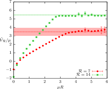
Thus we expect that the subtracted static potentials approach the asymptotic values
| (35) |
With the fit-values and we find
| (36) |
Fig. 5 (Right panel) shows the rescaled potentials for charges in the fundamental representations together with the asymptotic values (36) extracted from the glue-lump correlators. At fixed coupling both potentials flatten exactly at separations of the charges where the energy stored in the flux tube is twice the glue-lump energy.


Fig. 6 shows the local string tensions in the two fundamental representations and their ratio. Although more gluons (three instead of one) are involved we see clearly that the string connecting charges in the adjoint representation breaks earlier than the string connecting charges in the defining representation.
6 4-dimensional Gauge-Higgs model
The lattice action (9) depends on the inverse gauge coupling and the hopping parameter which is proportional to the vacuum expectation value of the Higgs field. For the gauge bosons decouple and the theory reduces to an -invariant nonlinear -model which shows spontaneous symmetry breaking down to at some critical value . The phase transition is of second order.
For the factor in the decomposition (4) is frozen and we end up with an gauge theory for the factor which shows a weak first order deconfinment transition. With respect to the unbroken subgroup the fundamental representations and branch into the following irreducible -representations:
| (37) |
The Higgs field branches into a scalar quark, scalar anti-quark and singlet with respect to . Similarly, a -gluon branches into a massless -gluon and additional gauge bosons with respect to . The latter eat up the the non-singlet scalar fields such that the spectrum in the broken phase consists of massless gluons, massive gauge bosons and one massive Higgs particle. If is lowered, in addition to the gluons of , the additional gauge bosons of with decreasing mass begin to participate in the dynamics. Similarly as dynamical quarks and anit-quarks in QCD, they transform in the representations and of and thus explicitly break the center symmetry. As in they are expected to weaken the deconfinement phase transition. Thus it has been conjectured in [3] that there may exist a critical endpoint where the deconfinement transition disappears. For we recover gluodynamics with a first order deconfinement phase transition.
We measure the Polyakov loop as an (approximate) order parameter for confinement and investigate the corresponding critical curve in the - plane. For large the confinement phase in is characterised by . If in the deconfinement phase the centre symmetry of the remaining is broken then the ambiguity of measuring is fixed by choosing the Polyakov loop that points into the -direction of . Technically this is achieved by taking . The results are shown in Fig. 7 (Left panel). We observe that on the small lattice the Polyakov loop jumps along a continuous line connecting the deconfinement transitions of pure and pure gluodynamics. This points to a continuous line of deconfinement transitions all the way from to . To see whether this is indeed the case we performed high-precision simulations on larger lattices. A careful analyses of histograms and suszeptibilies for Polyakov loops and the Higgs part of the action confirm the results on the small lattice. Unfortunately a rather small region in parameter space is left where we cannot resolve the order of the transition. In this small region there could exist a crossover from the confining to the deconfining phase.


On a larger () lattice we calculate also the full phase diagram including the Higgs transition (Fig. 7, Right panel). Phase transitions are obtained by observing susceptibility peaks in the Polyakov loop and the Higgs part of the action. We also investigate the order of the confinement-deconfinement transition using the histogram method for the Polyakov loops. For the order of the Higgs transition line we consider the finite size scaling of () for lattices up to . With the data obtained so far the point where the second order transition may turn into a crossover cannot be determined reliably. If the triple point exists then an extrapolation to the point where the confining phase meets both deconfining phases leads to the couplings and .
7 Conclusions
In the present work we implemented an efficient and fast LHMC algorithm to simulate gauge theory in three and four dimensions. In addition we implemented a slightly modified Lüscher-Weisz multi-step algorithm with exponential error reduction to measure the static potentials for charges in various representations. The accurate results in dimensions show that the static potentials show Casimir scaling on intermediate scales within a few percent statistical errors. Thus we conclude that in dimensional gluodynamics the Casimir scaling violations of the string tensions are small for all charges in the representations with dimensions and .
For larger separations we detect string breaking in the two fundamental representations exactly at the expected scale where the energy stored in the flux tube is sufficient to create two glue-lumps. To confirm this expectation we calculated masses of glue-lumps associated with static charges in the fundamental representations. Here, close to the string breaking distance, systematic Casimir scaling violations show up (for a more detailed discussion see [6]).
In dimensions we explored the full phase diagram of the Gauge Higgs model. We found a line of first order phase transitions connecting and gluodynamics and a line of second order phase transitions separating the deconfinement phase from the deconfinement phase. Unfortunately we cannot exclude the existance of a small crossover region near the would-be tripel point of the system. Details on the Gauge Higgs model will be published in a follow up paper.
Acknowledgments.
The author thanks Andreas Wipf and Christian Wozar for collaboration and support. Helpful discussions with Philippe de Forcrand, Christof Gattringer, Kurt Langfeld, Uwe-Jens Wiese and Stefan Olejnik are gratefully acknowledged. This work has been supported by the DFG under GRK 1523.References
- [1] K. Holland, M. Pepe and U. J. Wiese, The deconfinement phase transition of Sp(2) and Sp(3) Yang-Mills theories in 2+1 and 3+1 dimensions, Nucl. Phys. B694 (2004) 35.
- [2] K. Holland, P. Minkowski, M. Pepe and U. J. Wiese, Exceptional confinement in G(2) gauge theory, Nucl. Phys. B668 (2003) 207.
- [3] M. Pepe and U. J. Wiese, Exceptional Deconfinement in G(2) Gauge Theory, Nucl. Phys. B768 (2007) 21.
- [4] L. Liptak and S. Olejnik, Casimir scaling in G(2) lattice gauge theory, Phys. Rev. D78 (2008) 074501.
- [5] J. Greensite, The confinement problem in lattice gauge theory, Prog. Part. Nucl. Phys. 51 (2003) 1.
- [6] B. Wellegehausen, A. Wipf and C. Wozar, Casimir Scaling and String Breaking in G(2) Gluodynamics, CITATION = HEP-LAT/1006.2305
- [7] A. J. Macfarlane, The sphere S(6) viewed as a G(2)/SU(3) coset space, Int. J. Mod. Phys. A17 (2002) 2595.
- [8] P. Marenzoni, L. Pugnetti and P. Rossi, Measure Of Autocorrelation Times Of Local Hybrid Monte Carlo Algorithm For Lattice QCD, Phys. Lett. B 315 (1993) 152.
- [9] M. Luescher and P. Weisz, Locality and exponential error reduction in numerical lattice gauge theory, JHEP 0109 (2001) 010.